


ABSTRACT
We determine basic thermodynamic and transport properties of hydrogen–helium–water mixtures for the extreme conditions along Jupiter's adiabat via ab initio simulations, which are compiled in an accurate and consistent data set. In particular, we calculate the electrical and thermal conductivity, the shear and longitudinal viscosity, and diffusion coefficients of the nuclei. We present results for associated quantities like the magnetic and thermal diffusivity and the kinematic shear viscosity along an adiabat that is taken from a state-of-the-art interior structure model. Furthermore, the heat capacities, the thermal expansion coefficient, the isothermal compressibility, the Grüneisen parameter, and the speed of sound are calculated. We find that the onset of dissociation and ionization of hydrogen at about 0.9 Jupiter radii marks a region where the material properties change drastically. In the deep interior, where the electrons are degenerate, many of the material properties remain relatively constant. Our ab initio data will serve as a robust foundation for applications that require accurate knowledge of the material properties in Jupiter's interior, e.g., models for the dynamo generation.
Export citation and abstract BibTeX RIS
1. INTRODUCTION
The detection of a great number of Jupiter-mass planets has boosted the interest in the physics of giant planets. Fundamental questions are related to their formation, evolution, and present structures including internal flow dynamics and magnetic field generation (Stevenson 1982; Guillot 2005; Jones et al. 2011). Little is known about the extrasolar planets and even our knowledge about Jupiter is still incomplete. The latter should improve considerably with the arrival of NASA's Juno mission at Jupiter in 2016 (Matousek 2007).
While progress has been achieved in explaining the overall shape of Jupiter's dipole-dominated field geometry (Christensen & Aubert 2006; Wicht & Tilgner 2010; Stanley & Glatzmaier 2010; Schubert & Soderlund 2011), basic properties, such as the observed flow patterns in the atmosphere (Heimpel et al. 2005; Vasavada & Showman 2005; Kaspi et al. 2009; Gastine & Wicht 2012), still await explanations that are consistent with planetary structure and dynamo models. So far, many of these models use rather gross simplifying assumptions about the interior structure and material properties, partially for numerical convenience but also because of the lack of adequate data. The knowledge of the properties of matter inside Jupiter is thus very important for both interior structure and magnetic field models.
In the past decade, enormous progress has been made in high-pressure experimental techniques (see, e.g., Knudson et al. 2004; Fortov et al. 2007; Celliers et al. 2010; Subramanian et al. 2011; Knudson et al. 2012), so that the Mbar pressure range can now be probed even for the light elements H and He. Simultaneously, the behavior of hydrogen and helium under extreme conditions has been investigated using ab initio simulations (see, e.g., Desjarlais 2003; Militzer 2006, 2009; Vorberger et al. 2007; Kietzmann et al. 2007; Holst et al. 2008, 2011; Stixrude & Jeanloz 2008; Lorenzen et al. 2009, 2010, 2011; Morales et al. 2009, 2010; Caillabet et al. 2011; Hamel et al. 2011). The predictions that can be made with the ab initio simulation technique are generally in very good agreement with experiments. Furthermore, the method allows one to examine extreme thermodynamic states deep inside Jupiter that cannot yet be generated in the laboratory.
In spite of all of the progress, no data set that has been derived consistently using a single method for the thermophysical properties, i.e., the equation of state (EOS), as well as for transport properties, is yet available for the interior conditions of Jupiter. While the chemical model EOS of Saumon et al. (1995) for H and He has had wide application in planetary physics, the electronic transport properties are usually approximated by interpolating between known limiting cases such as the fully ionized classical plasma (Spitzer & Härm 1953) and the degenerate quantum plasma (Ziman 1961). For instance, feasible interpolation formulae were given by Hubbard (1966), Lee & More (1984), Ichimaru & Tanaka (1985), and Röpke & Redmer (1989). Simple estimations for the thermal diffusivity and viscosity of hydrogen–helium mixtures exist as well (Stevenson & Salpeter 1977).
The aim of the present paper is to provide, for the first time, an accurate data set for the electrical conductivity σ, thermal conductivity λ, shear viscosity η, longitudinal viscosity η', the self-diffusion coefficients of hydrogen DH and helium DHe, heat capacities cp and cv, thermal expansion coefficient α, isothermal compressibility κT, sound velocity cs, and Grüneisen parameter γ at conditions along Jupiter's adiabat. Our data are obtained entirely from ab initio simulations (see Gillan et al. 2006; Hafner 2008 for reviews). This is the same method that has recently been used to calculate an improved hydrogen EOS and corresponding new Jupiter models and adiabats (Nettelmann et al. 2012).
We expect that this work will provide a robust set of material data that can be applied in models of Jupiter's magnetic field and internal flow dynamics (Kirk & Stevenson 1987; Heimpel et al. 2005). In such applications, our results would enter several of the dimensionless quantities (characteristic numbers) that can be defined, see, e.g., Table 2 in the review of Schubert & Soderlund (2011) for a compilation of those. So far, these models rely on relatively rough estimates of the quantities mentioned above. Therefore, the derivation of consistent ab initio data for the thermodynamic and transport properties of H/He under extreme conditions is a very beneficial effort.
Our paper is arranged as follows. Sections 2 and 3 describe the ab initio simulation method for the EOS data and the interior model for Jupiter and contain results for the Jupiter adiabat, basically referring to the recent work of Nettelmann et al. (2012). Our results for the thermodynamic material properties cp, cv, α, κT, cs, and γ are presented in Section 4. The theoretical method for computing the transport properties σ, λ, η, η', DH, and DHe is described in Section 5 while Section 6 contains the respective results for the transport properties. We summarize our results and discuss their potential impact on future flow and dynamo models in Section 7.
2. AB INITIO SIMULATIONS FOR THE EOS DATA
In this paper, we calculate the material properties along Jupiter's adiabat. Therefore, accurate EOS data for the main components (hydrogen, helium, and heavy elements) as well as a state-of-the-art interior model are necessary. The underlying EOS data—a linear-mixture EOS of hydrogen, helium, and water—that will serve in the calculations of material properties in Section 4 have previously been used to calculate a series of Jupiter models (Nettelmann et al. 2012). Although the heavy elements, represented by water, occur only in very small quantities in Jupiter's envelope, their contribution to the total mass density ϱ must be taken into account in the complete EOS.
The EOS data for helium and water are the same as described in Nettelmann et al. (2008). The EOS of hydrogen, however, has been refined (H-REOS.2), which is explained in more detail in Nettelmann et al. (2012). For the sake of clarity, we repeat here the characteristics of the ab initio simulation method as well as numerical details of the calculations for hydrogen. Because of its high concentration in Jupiter the behavior of hydrogen dominates the properties of the complete EOS. Note that ab initio EOS data cover the pressure region above ∼0.08 Mbar for H, ∼0.1 Mbar for He, (Kietzmann et al. 2007), and ∼0.1 Mbar for H2O (French et al. 2009); see also Figures 1–3 in Nettelmann et al. (2008). The EOS of the mixture is obtained by the additive volume rule (Chabrier et al. 1992), implying a linear superposition of the single materials' EOS which neglects interactions between the different materials. As a result, combined data tables for the thermal and the caloric EOS were generated from which all thermodynamic quantities of interest can be gained via interpolation and differentiation.
The ab initio simulation method allows a quantum-statistical treatment of the electrons within the framework of finite-temperature density functional theory (FT-DFT) (Mermin 1965) in combination with classical molecular dynamics (MD) simulations for the ions in the Born–Oppenheimer approximation. The Vienna Ab initio Simulation Package (VASP; Kresse & Hafner 1993, 1994; Kresse & Furthmüller 1996) was used to calculate the EOS of hydrogen (Nettelmann et al. 2012). The exchange-correlation functional is the fundamental physical input in FT-DFT calculations, and the approximation of Perdew et al. (1996, hereafter PBE), which yields generally good results for the thermodynamic properties of warm dense matter, has been used; see, e.g., Holst et al. (2008), Knudson et al. (2008), Caillabet et al. (2011), and French et al. (2009).
From the FT-DFT algorithm, the forces on the ions are derived via the Hellmann–Feynman theorem at each MD time step. This procedure is repeatedly performed in a cubic simulation box with periodic boundary conditions for several thousand MD time steps. The ion temperature is controlled with a Nosé thermostat (Nosé 1984). In the case of hydrogen, typical simulations were about 5 ps long with time steps ranging from 0.1 to 1 fs.
Excellent convergence of the results was ensured with several checks with respect to the particle number, the sets used for the evaluation of the Brillouin zone, as well as the employed pseudopotentials and their respective energy cutoff for the plane-wave basis set. Projector-augmented wave (PAW) pseudopotentials (Blöchl 1994; Kresse & Joubert 1999) were used at all considered densities with a converged energy cutoff of 1200 eV. The EOS simulations for H were performed with 256 particles and the Baldereschi mean-value  point (Baldereschi 1973), as in earlier work (Holst et al. 2008; Lorenzen et al. 2010; Holst et al. 2011).
Since the ions are treated as classical particles within an FT–DFT–MD simulation, the heat capacities of molecular gases are usually overestimated (French & Redmer 2009), so that a quantum-mechanical correction to the caloric EOS u(ϱ, T) with respect to the molecular vibrations had to be made afterward; see Nettelmann et al. (2012) for details.
The ab initio simulation method as described here is also used in the calculations for the present paper.
3. JUPITER MODELS AND ADIABAT
The work presented here relies on the linear-mixing EOS described above and on Jupiter models constructed by Nettelmann et al. (2012). Here we give only a brief summary of their key features. The Jupiter models have two adiabatic homogeneous envelopes and a core of rocks. These models reproduce the measured values of the planet mass MJ; the equatorial radius Req = 7.1492 × 10⁷ m; the atmospheric mass abundances of helium and heavy elements; the angular velocity; the three lowest-order gravitational moments J2, J4, J6; and the 1 bar temperature T1 which determines the entropy of the outer envelope, within their observational error bars. The models have a mean He:H mass ratio Y = MHe/(MHe + MH) = 0.275, while the He abundance chosen in the outer envelope, Y1 = 0.238, is in agreement with the measured one in the atmosphere. The two envelopes are also allowed to differ in their respective mass fractions of heavy elements Z1 and Z2, which are used as adjusting parameters to match J2 and J4, respectively.
In this paper, we select two representative models from Nettelmann et al. (2012). In particular, model J11-4a has a transition pressure between the envelopes of P1-2 = 4 Mbar, resulting in Mcore = 7.57 M⊕, Z1 = 0.030, Z2 = 0.090, Y2 = 0.291, and R(P1-2) = 0.736RJ, while model J11-8a has P1-2 = 8 Mbar, Mcore = 3.56 M⊕, Z1 = 0.038, Z2 = 0.128, Y2 = 0.311, and R(P1-2) = 0.629RJ, where RJ = 6.9894 × 10⁷ m is Jupiter's mean radius.
Originally, the adiabats for these models were derived via a thermodynamic integration scheme; see Nettelmann et al. (2012). Here we recalculate the adiabats with the following relation:
When keeping all model parameters from Nettelmann et al. (2012) constant, this yields slightly different results for p and T because the procedure is more sensitive to the local derivatives of the EOS data. In addition, the new adiabat is smoother and we believe that it is more appropriate for our special purpose of deriving material properties. The maximum deviation between the new and the original adiabats is 5% for both P(R) and T(R) and occurs mainly in the dissociation regime near 0.9RJ. The density profile remains unchanged.
The internal profiles P(R), T(R), and ϱ(R) of the respective models are shown in Figure 1. As can be seen, the pressure and temperature profiles are relatively insensitive to details of the model assumptions. This property allows us to define a general Jupiter adiabat in P–T space. Therefore, we mainly focus on the Jupiter model J11-8a in the following.
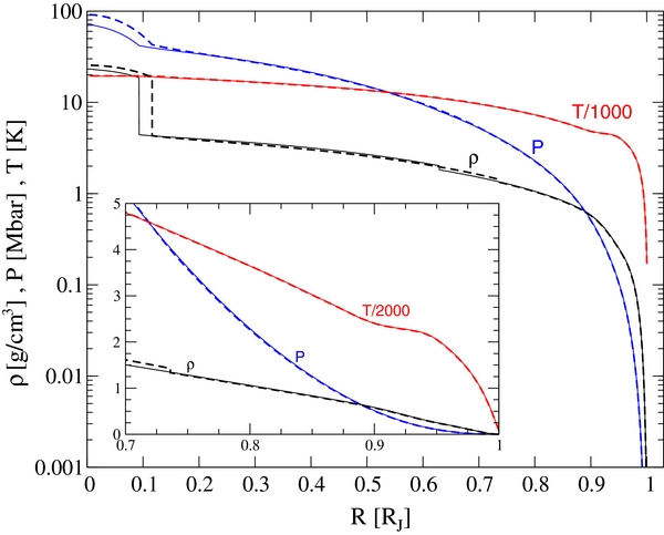
Figure 1. Interior profiles of pressure (blue), temperature (red), and mass density (black) for the two representative Jupiter models J11-4a (dashed) and J11-8a (thin solid). The density has a jump at the transition pressure between the envelopes. Inset: the transit region between the metallic inner region and the molecular outer part.
Download figure:
Standard image High-resolution imageThe density profiles displayed here may serve to set the average density for the flow and dynamo models which apply the Boussinesq approximation (Braginsky & Roberts 1995; Heimpel & Aurnou 2007; Wicht & Tilgner 2010) or the density gradient in the anelastic approximation of more advanced models (Kaspi et al. 2009; Stanley & Glatzmaier 2010; Jones et al. 2011; Gastine & Wicht 2012).
4. THERMODYNAMIC MATERIAL PROPERTIES
In this section, we outline the calculation of thermodynamic material properties and present the corresponding results. We have determined these quantities from the linearly mixed ab initio EOS by differentiation in the vicinity of the Jupiter adiabat. The major results are listed in Table 1.
Table 1. Thermodynamic Material Properties in Jupiter (Model J11-8a)
| R | ϱ | T | P | cp | cv | α | κT | cs | γ |
|---|---|---|---|---|---|---|---|---|---|
| (RJ) | (g cm−3) | (K) | (GPa) | (kJ gK−1) | (kJ gK−1) | (1 K−1) | (1 GPa−1) | (km s−1) | |
| 0.0923 | 4.42 | 19500 | 4180 | 1.33 × 10⁻² | 1.25 × 10⁻² | 4.85 × 10⁻⁶ | 1.25 × 10⁻⁴ | 44.03 | 0.705 |
| 0.196 | 3.99 | 18000 | 3410 | 1.36 × 10⁻² | 1.27 × 10⁻² | 5.43 × 10⁻⁶ | 1.53 × 10⁻⁴ | 41.89 | 0.707 |
| 0.350 | 3.39 | 16000 | 2460 | 1.36 × 10⁻² | 1.27 × 10⁻² | 6.58 × 10⁻⁶ | 2.13 × 10⁻⁴ | 38.64 | 0.737 |
| 0.478 | 2.80 | 14000 | 1640 | 1.36 × 10⁻² | 1.26 × 10⁻² | 7.82 × 10⁻⁶ | 3.10 × 10⁻⁴ | 35.23 | 0.728 |
| 0.584 | 2.26 | 12000 | 1030 | 1.37 × 10⁻² | 1.25 × 10⁻² | 1.04 × 10⁻⁵ | 4.79 × 10⁻⁴ | 31.83 | 0.782 |
| 0.629 | 2.02 | 11000 | 800 | 1.37 × 10⁻² | 1.24 × 10⁻² | 1.22 × 10⁻⁵ | 6.07 × 10⁻⁴ | 30.10 | 0.823 |
| 0.629 | 1.82 | 11000 | 800 | 1.52 × 10⁻² | 1.37 × 10⁻² | 1.22 × 10⁻⁵ | 6.14 × 10⁻⁴ | 31.49 | 0.807 |
| 0.680 | 1.60 | 10000 | 600 | 1.49 × 10⁻² | 1.34 × 10⁻² | 1.38 × 10⁻⁵ | 8.08 × 10⁻⁴ | 29.34 | 0.802 |
| 0.770 | 1.20 | 8000 | 300 | 1.49 × 10⁻² | 1.33 × 10⁻² | 1.90 × 10⁻⁵ | 1.52 × 10⁻³ | 24.82 | 0.781 |
| 0.852 | 0.824 | 6000 | 120 | 1.45 × 10⁻² | 1.29 × 10⁻² | 2.83 × 10⁻⁵ | 3.64 × 10⁻³ | 19.38 | 0.737 |
| 0.890 | 0.638 | 5000 | 64 | 1.47 × 10⁻² | 1.37 × 10⁻² | 3.09 × 10⁻⁵ | 7.09 × 10⁻³ | 15.44 | 0.501 |
| 0.900 | 0.581 | 4800 | 51 | 1.57 × 10⁻² | 1.48 × 10⁻² | 3.12 × 10⁻⁵ | 9.11 × 10⁻³ | 14.15 | 0.402 |
| 0.908 | 0.531 | 4700 | 42 | 1.73 × 10⁻² | 1.66 × 10⁻² | 2.86 × 10⁻⁵ | 1.15 × 10⁻² | 13.04 | 0.292 |
| 0.918 | 0.464 | 4600 | 32 | 1.93 × 10⁻² | 1.88 × 10⁻² | 2.72 × 10⁻⁵ | 1.60 × 10⁻² | 11.74 | 0.208 |
| 0.930 | 0.380 | 4500 | 23 | 2.06 × 10⁻² | 1.99 × 10⁻² | 3.76 × 10⁻⁵ | 2.47 × 10⁻² | 10.50 | 0.215 |
| 0.940 | 0.312 | 4400 | 16 | 1.87 × 10⁻² | 1.73 × 10⁻² | 5.97 × 10⁻⁵ | 3.57 × 10⁻² | 9.87 | 0.323 |
| 0.952 | 0.240 | 4000 | 9.6 | 1.59 × 10⁻² | 1.34 × 10⁻² | 9.27 × 10⁻⁵ | 5.75 × 10⁻² | 9.28 | 0.503 |
| 0.964 | 0.177 | 3500 | 5.0 | 1.54 × 10⁻² | 1.22 × 10⁻² | 1.36 × 10⁻⁴ | 1.15 × 10⁻¹ | 7.86 | 0.526 |
| 0.972 | 0.132 | 3000 | 2.7 | 1.40 × 10⁻² | 1.12 × 10⁻² | 1.68 × 10⁻⁴ | 2.31 × 10⁻¹ | 6.41 | 0.498 |
| 0.980 | 0.0848 | 2500 | 1.2 | 1.34 × 10⁻² | 1.03 × 10⁻² | 2.58 × 10⁻⁴ | 6.23 × 10⁻¹ | 4.97 | 0.494 |
| 0.986 | 0.0497 | 2000 | 0.45 | 1.29 × 10⁻² | 9.55 × 10⁻³ | 3.89 × 10⁻⁴ | 1.78 | 3.90 | 0.470 |
| 0.994 | 0.0113 | 1000 | 0.0434 | 1.22 × 10⁻² | 8.50 × 10⁻³ | 9.50 × 10⁻⁴ | 21.97 | 2.40 | 0.453 |
Notes. The number of digits does not necessarily correspond to the actual error bar in all cases. The double values at 11000 K are either from the inner or the outer envelope. The respective boundary is also indicated by a separating line. It is RJ = 6.9894 × 10⁷ m.
Download table as: ASCIITypeset image
4.1. Definitions
To calculate the thermal expansion coefficient α, the isothermal compressibility κT, the specific heat capacities for constant volume (or density), cv, and for constant pressure, cp, we use the following definitions:
We use cubic spline interpolations to generate smooth curves of P(ϱ, T) and u(ϱ, T) from the EOS data tables. The material properties are then derived via analytic differentiation of the spline polynomials.
Several other material properties can be expressed as functions of the quantities given above. For example, the sound velocity is determined from the heat capacities and the isothermal compressibility via
The Grüneisen parameter is given by
4.2. Results
4.2.1. Specific Heat Capacities, Isothermal Compressibility, and Thermal Expansion Coefficient
The numerical results for cp, cv, κT, and α are shown in Figure 2. Starting at RJ, the heat capacity cv increases inward until reaching a maximum at ∼0.9RJ (i.e., ∼0.5 Mbar) which is caused by the dissociation of hydrogen molecules. The isobaric heat capacity cp shows a similar behavior as cv but is larger, as is required by a thermodynamic stability condition. For R < 0.85RJ, cv and cp remain nearly constant right down to the core–mantle boundary, except for a jump at the transition pressure (here 8 Mbar) due to the different abundances of helium and heavy elements in the layers. Although H has a larger heat capacity than He, it is less abundant in the lower layer, which leads to a smaller heat capacity of the mixture.

Figure 2. Thermodynamic material properties along Jupiter's adiabat for the model J11-8a: specific heat capacities cv (red dashed) and cp (red solid), isobaric expansion coefficient α (black solid), isothermal compressibility κT (black dashed), and cp − cv (blue solid); see Equation (5). The discontinuities at 0.63 RJ are due to different material abundances in the layers.
Download figure:
Standard image High-resolution imageThe thermal expansion coefficient α, together with κT, T, and ϱ, determines the difference between cp and cv; see Equation (5). The temperature and the density increase monotonously with the depth while κT decreases. Only the expansion coefficient α has a local extremum, which occurs exactly in the dissociation regime. There, the difference between the heat capacities becomes very small. The smooth behavior of all quantities in the second term of Equation (5) leads to compensating effects and hence to parallel slopes of cp and cv.
A first-order liquid–liquid phase transition has been predicted in hydrogen for temperatures below 2000 K (Morales et al. 2010; Lorenzen et al. 2010), which is accompanied by the abrupt dissociation of hydrogen molecules. While the isentrope is well above the critical point of this first-order transition, Figure 3 suggests that an extrapolation of the 50% dissociation line (Tamblyn & Bonev 2010) to higher temperatures intersects with the Jupiter adiabat. The heat capacities cp and cv have a maximum in that particular region, which reflects the additional energy required to break the intramolecular bonds.
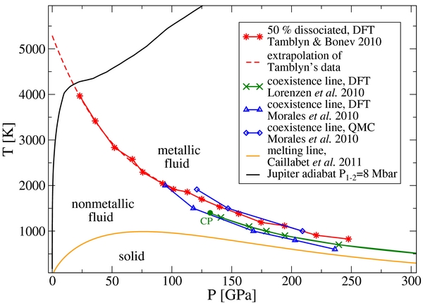
Figure 3. Phase diagram of hydrogen with the Jupiter adiabat. The data are taken from Tamblyn & Bonev (2010), Lorenzen et al. (2010), Morales et al. (2010), and Caillabet et al. (2011).
Download figure:
Standard image High-resolution image4.2.2. Sound Velocity and Grüneisen Parameter: Consequences for the Adiabat
Figure 4 shows that cs rises with depth within both envelopes as the interior becomes warmer but also increasingly degenerate. When dissociation occurs at ∼0.9RJ, cv rises steeper than cp, and the increase of cs with depth is attenuated. At the internal layer boundary, the discontinuous rise in mass density maps onto a respective decrease in cs, which can be seen in Figure 4.

Figure 4. Sound velocity (upper panel) and Grüneisen parameter (lower panel) along Jupiter's adiabat for the model J11-8a. The discontinuities at 0.63 RJ are due to different material abundances in the layers.
Download figure:
Standard image High-resolution imageIn the deep interior, the value of the Grüneisen parameter is almost constant and close to the ideal Fermi-gas value of 2/3. This behavior changes drastically in the dissociation regime, where the Grüneisen parameter drops to about 0.2. The reason for this is the minimum in α and the maximum in cv which add to each other; see Equation (7). However, the effect is only local and outside of ∼0.95RJ, the Grüneisen parameter tends to approach a value close to 0.4, which is characteristic for a classical diatomic ideal gas without vibrational excitations.
According to Equation (1), the Grüneisen parameter determines the slope of the adiabat. The flattening of the adiabat in the dissociation regime (see Figure 3) is thus a direct consequence of the pronounced minimum in γ.
5. TRANSPORT PROPERTIES: THEORY
The calculation of transport properties with the FT-DFT-MD method involves the application of linear response theory (Kubo 1957) and is much more demanding than pure EOS calculations. All transport properties are derived from FT-DFT-MD simulations for a hydrogen–helium mixture with representative concentrations. We employ again the VASP program package (Kresse & Hafner 1993, 1994; Kresse & Furthmüller 1996). The influence of heavier elements is neglected here because of their small particle abundances in the envelopes of Jupiter.
Due to the Born–Oppenheimer approximation we have to treat the contributions of the electrons and nuclei separately in the conductivity calculations. In the case of the electrical conductivity, the electronic contribution σe is much larger than that of the ions σi. The reason for this is that, once the system ionizes, the free electrons are much more mobile than the nuclei because of their large mass difference. Significant ionic conductivity, e.g., due to proton hopping as in warm dense water (French et al. 2011), can be ruled out because no charge transfer occurs between hydrogen and helium when all electrons are bound. Thus, we can safely approximate the total electrical conductivity as σ = σe.
In contrast, the electronic contribution to the thermal conductivity of the electrons λe is not always larger than the contributions of the ions λi. In particular, the molecular region of the phase diagram, where the electrons are bound and the energy is transported via intermolecular collisions, shows a very small λe. Therefore, the total thermal conductivity is generally given by the sum of both terms, λ = λe + λi.
5.1. Viscosities
The viscosities are governed by the motion of the nuclei so that the contribution of free electrons does not need to be considered for these quantities (Bertolini et al. 2007; Bernu & Vieillefosse 1978).
Both shear and longitudinal viscosities were determined from FT–DFT–MD simulations for H–He mixtures using the standard PAW pseudopotentials (Blöchl 1994; Kresse & Joubert 1999) and a cutoff energy of 1200 eV. We employ the PBE exchange-correlation functional (Perdew et al. 1996). An ensemble of 108 hydrogen and 10 helium atoms was simulated to represent the mean helium concentration of Y = 0.275. Depending on the density, either the 2 × 2 × 2 Monkhorst–Pack  -point set (Monkhorst & Pack 1976) or the Balderschi point (Baldereschi 1973) was chosen to ensure the convergence of the pressure tensor.
The dynamic shear viscosity η was then derived within the standard linear response approach (Kubo et al. 1991; Allen & Tildesley 1989; Alfè & Gillan 1998) which requires the calculation of a time integral over the autocorrelation function of the off-diagonal components pij of the pressure tensor,
In the above equation, Ω is the volume of the simulation box and kB is Boltzmann's constant. In the same way, the longitudinal viscosity η' was calculated from the autocorrelation function of the diagonal elements pi of the pressure tensor,
For each data point, a simulation with 80000 to 140000 time steps, with time-step sizes of 0.2 or 0.3 fs, was performed to attain a statistical uncertainty for η and η' of better than 10% in most cases. In addition, several simulations were done to test the convergence with respect to all numerical parameters listed here and to rule out potential disturbances by the thermostat.
5.2. Electrical and Thermal Conductivity: Electronic Contribution
5.2.1. Onsager Coefficients
As a first step to obtain electrical and thermal conductivities, we performed FT–DFT–MD simulations to get ensembles of equilibrated ion configurations. Then we calculated the frequency-dependent Onsager coefficients for electron transport in subsequent static FT–DFT runs for 20–100 ion configurations taken from each of the simulations. The respective results were then averaged. Expressions for the Onsager coefficients Lmn(ω) were derived by Holst et al. (2011) in the framework of linear response theory. They read
where ω is the frequency, q = −e and me are the charge and mass of an electron, he is the enthalpy per electron, Ekμ and fkμ are the eigenvalue and Fermi occupation number of the Bloch state  , and
, and  are matrix elements with the momentum operator.
The coefficient L11(ω) is also known as the frequency-dependent Kubo–Greenwood formula (Kubo 1957; Greenwood 1958). The static electrical conductivity is obtained via

Likewise, the thermal conductivity is calculated via the relation
These calculations were performed with 256 electrons in the simulation box (considering several H–He ion concentrations) and, depending on the density, different  -point sets (Baldereschi 1973; Monkhorst & Pack 1976). We use the standard PAW pseudopotentials for H and He with a plane-wave cutoff energy of 400 eV or higher. Again, several tests were made to confirm that the choice of these parameters yields well-converged Onsager coefficients.
5.2.2. Exchange-correlation Functional
The selection of the exchange-correlation functional, which determines the  and Ekμ, is a delicate matter in electronic conductivity calculations with FT–DFT. The PBE functional, which is used in all MD simulations here, usually underestimates the fundamental electronic band gap considerably, so that the conductivities are too high. To overcome this problem, we use the hybrid functional of Heyd, Scuseria, and Ernzerhof (HSE; Heyd et al. 2003, 2006), which reproduces the band gaps of semiconductors much more accurately (Heyd et al. 2005; Paier et al. 2006), in most of the calculations of the Onsager coefficients, Equation (10). Hybrid functionals require the calculation of the nonlocal Fock-exchange integral, which involves significantly higher computational efforts. We use the HSE functional with a screening parameter of μs = 0.2 Å−1.
To illustrate the effect of the exchange-correlation functional, we plot the ratios of the conductivities that were obtained with each of these functionals (HSE vs. PBE) in Figure 5. In the molecular regime, the electronic contributions to both the electrical and the thermal conductivity are overestimated by up to two orders of magnitude using the PBE functional, whereas this effect is less important in the metallic regime. Nevertheless, the PBE functional gives the correct qualitative trends of the metal-to-nonmetal transition in the H–He mixture, similar to earlier work on high-pressure water (French et al. 2010).

Figure 5. Ratios of the electrical (σe) and thermal conductivities (λe) along the Jupiter adiabat, obtained with the HSE and the PBE exchange-correlation functionals.
Download figure:
Standard image High-resolution image5.3. Electrical and Thermal Conductivities: Ionic Contribution
The ions (nuclei) are propagated as classical particles in our simulations. Therefore, we can apply classical Green–Kubo relations, as in the viscosity calculations, to determine their contribution to the conductivities. Keeping in mind the introductory considerations of Section 5, one can estimate that the electrical conductivity of the electrons σe is much higher than that of the ions, σi, and we can neglect the latter.
In the same way, the electronic contribution to the thermal conductivity λe is also much higher than λi once ionization becomes significant. Thus, λi is only important in the nonmetallic region, and we can treat the ions as effectively neutral particles (due to the formation of He atoms and H2 molecules) when calculating their contribution to the thermal conductivity. Consequently, the thermal conductivity of the ions can be calculated with the equation (Allen & Tildesley 1989)
Regrettably, a rigorous way to express the generalized heat current  within FT–DFT–MD is yet unknown, so that we have to make additional but reasonable approximations here. We accomplish this by mapping the effective interactions between the nuclei in FT–DFT onto classical pair potentials. This allows us to adopt a well-known expression for Jq that is commonly applied in classical MD simulations. It is defined (Hansen & McDonald 1976; de Groot & Mazur 1984; Allen & Tildesley 1989) as
where N is the total number of ions,  and Ek are velocity and energy of the particle k, and 〈hk〉 is its mean enthalpy, respectively. The energy per particle is given by
The potentials Vkj and forces  shall depend only on the distances
  between the particles k and j. The last task is to obtain the effective interaction potentials between the species. Here we use a first-order approximation and express the pair potentials Vab(r) and forces
  between the species a and b through radial pair correlation functions gab(r) via

All gab(r) can be easily calculated from FT–DFT–MD simulation data. The mean enthalpy of a particle from the species a follows without further approximation and reads (Hansen & McDonald 1976)
The virial contribution to 〈ha〉 vanishes.
Such an approach, although it is not rigorously ab initio, offers significant advantages over using only the kinetic energy in the heat current or, much simpler, expressing the thermal conductivity through diffusion coefficients. Even though it has the potential to be improved, we checked that the present level is sufficient to yield reasonable thermal conductivities for the H–He mixture; at low densities they agree with extrapolated experimental data for hot gaseous hydrogen (Assael et al. 2011).
We used the same simulations that served to calculate the viscosities (108 hydrogen and 10 helium atoms, Y ≈ 0.275) to obtain λi. Due to the approximations made here, we estimate that the overall accuracy of the λi is within a factor of two or better.
5.4. Self-diffusion Coefficients
The self-diffusion coefficients of hydrogen DH and helium DHe were calculated with the following Green–Kubo formula:
In practice, the calculation of self-diffusion coefficients requires less extensive simulations than viscosities or thermal conductivities. Consequently, the same simulation runs (with 108 hydrogen and 10 helium atoms, Y ≈ 0.275) were used here as well. We estimate that our diffusion coefficients are generally accurate within 5% to 20%, depending on the species and density.
6. TRANSPORT PROPERTIES: RESULTS
In the following, we present the results for the transport properties calculated at the thermodynamic states (P, T) along the Jupiter adiabat. The density ϱ and the heat capacity cp from Section 4 will also find application in this section. Our main results are compiled in Table 2. The error bars are mostly due to statistical fluctuations unless noted otherwise.
Table 2. Linear Transport Properties in Jupiter (Model J11-8a)
| R | σ | β | λ | κ | η | ν | η' | DH | DHe |
|---|---|---|---|---|---|---|---|---|---|
| (RJ) | (S m−1) | (m2 s−1) | (W Km−1) | (m2 s−1) | (mPa s) | (mm2 s−1) | (mPa s) | (mm2 s−1) | (mm2 s−1) |
| 0.0923 | 3.39 × 10⁶ | 0.235 | 1710 | 2.91 × 10⁻⁵ | 1.16 | 0.262 | 1.80 | 0.433 | 0.256 |
| 0.196 | 3.05 × 10⁶ | 0.261 | 1470 | 2.70 × 10⁻⁵ | 1.06 | 0.266 | 1.69 | 0.428 | 0.272 |
| 0.350 | 2.48 × 10⁶ | 0.321 | 1040 | 2.26 × 10⁻⁵ | 0.955 | 0.282 | 1.55 | 0.436 | 0.251 |
| 0.478 | 1.97 × 10⁶ | 0.404 | 721 | 1.89 × 10⁻⁵ | 0.830 | 0.296 | 1.30 | 0.450 | 0.254 |
| 0.584 | 1.48 × 10⁶ | 0.538 | 465 | 1.50 × 10⁻⁵ | 0.666 | 0.295 | 1.08 | 0.458 | 0.247 |
| 0.680 | 1.09 × 10⁶ | 0.730 | 283 | 1.19 × 10⁻⁵ | 0.500 | 0.313 | 0.92 | 0.468 | 0.229 |
| 0.770 | 7.20 × 10⁵ | 1.11 | 153 | 8.56 × 10⁻⁶ | 0.410 | 0.342 | 0.77 | 0.481 | 0.200 |
| 0.852 | 3.60 × 10⁵ | 2.21 | 59.6 | 4.99 × 10⁻⁶ | 0.297 | 0.360 | 0.49 | 0.471 | 0.179 |
| 0.890 | 1.46 × 10⁵ | 5.45 | 20.2 | 2.16 × 10⁻⁶ | 0.234 | 0.367 | 0.49 | 0.369 | 0.172 |
| 0.930 | 1.5 × 10³ | 5.3 × 10² | 2.78* | 3.55 × 10⁻⁷* | 0.140 | 0.368 | 0.99 | 0.274 | 0.260 |
| 0.952 | 6.6 × 100 | 1.2 × 10⁵ | 2.18* | 5.71 × 10⁻⁷* | 0.090 | 0.378 | 1.36 | 0.349 | 0.330 |
| 0.972 | 3.5 × 10⁻² | 2.3 × 10⁷ | 1.74* | 9.42 × 10⁻⁷* | 0.046 | 0.348 | ... | 0.410 | 0.400 |
| 0.980 | 3.5 × 10⁻⁴ | 2.3 × 10⁹ | 1.50* | 1.32 × 10⁻⁶* | 0.033 | 0.392 | ⋅⋅⋅ | 0.437 | 0.430 |
| 0.986 | 10−7 | 8 × 10¹² | 1.30* | 2.03 × 10⁻⁶* | 0.023 | 0.460 | ⋅⋅⋅ | 0.610 | 0.550 |
Notes. The number of digits does not necessarily correspond to the actual error bar in all cases, see figures and the text for details. Note that our data set for the longitudinal viscosities does not contain values for all radii. The values marked with "*" indicate that the ionic contributions λi and κi are dominant, see Sections 5 and 6 for further explanation. It is RJ = 6.9894 × 10⁷ m.
Download table as: ASCIITypeset image
6.1. Viscosities
We display the ab initio results for the dynamic shear η and longitudinal viscosity η' and the kinematic shear viscosity ν = η/ϱ along the Jupiter adiabat in Figure 6. Note that the density is taken from the linear-mixing EOS and therefore contains the mass fraction of heavy elements.
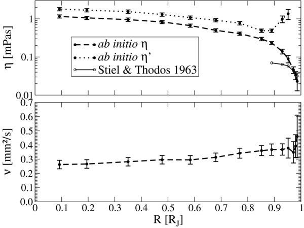
Figure 6. Upper panel: dynamic shear (dashed line) and longitudinal viscosity (dotted line) along Jupiter's adiabat. The thin solid line represents low-density values from Stiel & Thodos (1963). Lower panel: kinematic shear viscosity ν = η/ϱ.
Download figure:
Standard image High-resolution imageThe dynamic shear viscosity η decreases systematically with the radius. In the very outer regions, we find a plausible agreement with extrapolated low-density shear viscosities for pure hydrogen (Stiel & Thodos 1963). Many of our values are higher than the data of Stiel & Thodos (1963) because the H–He fluid becomes correlated in the interior of Jupiter, which leads to increased viscosities further inward.
The longitudinal viscosity η' decreases with the radius, but reaches a minimum near 0.9 RJ and then rises strongly as hydrogen molecules form in the outer envelope. In the metallic regime, the ratio between the longitudinal and shear viscosities approaches a value of η'/η ≈ 5/3, which is also frequently found in monoatomic fluids (Malbrunot et al. 1983; Hoheisel 1987). In molecular systems this ratio can be much higher (Emanuel 1990), which is consistent with our data. We did not calculate longitudinal viscosities outside of 0.95 RJ because the required convergence of the respective correlation functions could not be reached within our computational limits at such low densities.
The kinematic shear viscosity ν rises very slightly with the radius. It adopts an almost constant value of ∼0.3 mm2 s−1 in the entire interior; see Figure 6. Thus, a common qualitative approximation of a constant kinematic viscosity in the dynamo-generating region (Wicht & Tilgner 2010) is largely fulfilled. The respective values for the viscosities along the adiabat are given in Table 2.
6.2. Electrical Conductivity
First, we study the variation of the electronic contribution to the electrical and thermal conductivities with the helium concentration along the Jupiter adiabat. These quantities are potentially not as insensitive to the stoichiometry as η, λi, or diffusion coefficients and its influence needs some assessment.
Several calculations are performed for three different helium concentrations using the PBE functional. The general trends are displayed in Figure 7 and the correct absolute values for the conductivities can be obtained by scaling with the HSE:PBE ratios shown in Figure 5. In particular, we have chosen 216 hydrogen and 20 helium atoms to represent the mean helium fraction (Y ≈ 0.275), 222 hydrogen and 17 helium atoms (Y1 ≈ 0.238) for the outer layer, and 208 hydrogen and 24 helium atoms (Y2 ≈ 0.311) for the inner layer, respectively. The electrical and thermal conductivities of the H–He mixtures are mainly determined by the hydrogen subsystem. They decrease systematically with the helium concentration, similar to what was found by Lorenzen et al. (2011).

Figure 7. Dependence of the electrical (top) and the thermal (bottom) conductivity on the concentration of helium: Y1 ≈ 0.238 (dotted line), Y ≈ 0.275 (solid line), and Y2 ≈ 0.311 (dashed line). These calculations were performed with the PBE functional.
Download figure:
Standard image High-resolution imageFor all considered concentrations, the dependence of σe and λe on the helium abundance is relatively small. In a case where the influence of the helium concentration on the conductivity has to be accounted for, both this work and that of Lorenzen et al. (2011) can be used to scale the conductivities in the vicinity of the mean helium fraction. The discontinuity of the helium concentration at the layer boundary is a characteristic attribute of three-layer models by definition, however, it is relatively small in our models: from Y1 = 0.238 in the outer envelope to Y2 = 0.291 (J11-4a) or 0.311 (J11-8a) in the inner envelope. Therefore, and also due to the high computational demands, we restrict our following calculations with the HSE functional solely to the mean helium fraction (Y ≈ 0.275).
The main results for the electrical conductivity σ = σe and the magnetic diffusivity β = 1/μ0σ, where μ0 is the vacuum permeability, were obtained with the HSE functional (Heyd et al. 2003, 2006). They are displayed in Figure 8. The most prominent feature is the transition from nonmetallic to metallic-like conduction (σ ⩾ 2 × 10⁴ S m−1; see Redmer & Holst 2010) at about 0.9 RJ, which corresponds to a pressure level of 0.5 Mbar. The transition is continuous because Jupiter's adiabat lies above the critical point of the first-order liquid–liquid phase transition in hydrogen predicted by Morales et al. (2010) and Lorenzen et al. (2010); see Figure 3.

Figure 8. Upper panel: electrical conductivity along Jupiter's adiabat calculated with the HSE functional assuming a constant mean He fraction of Y ≈ 0.275. Comparison with different models and estimations is made (Stevenson & Salpeter 1977; Lee & More 1984; Röpke & Redmer 1989; Liu et al. 2008; Gómez-Pérez et al. 2010); see the text for further details. Lower panel: magnetic diffusivity β = 1/μ0σ along Jupiter's adiabat calculated with the HSE functional.
Download figure:
Standard image High-resolution imageVarious interpolation formulae have been constructed for the electrical conductivity based on limiting cases, e.g., the Spitzer theory (Spitzer & Härm 1953) for fully ionized classical plasmas, and the Ziman theory (Ziman 1961) for degenerate plasmas; see Röpke (1988) and Röpke & Redmer (1989). We compare our ab initio results with such transport theories developed for strongly coupled plasmas (Röpke & Redmer 1989; Lee & More 1984) assuming a fully ionized hydrogen plasma with a density that is equal to its partial density in our H–He mixture. We also compare our results with the model of Stevenson & Salpeter (1977) which takes into account the influence of helium. The formula of Stevenson & Salpeter (1977) is derived from the Ziman theory by employing hard sphere static structure factors. The model of Lee & More (1984) is based on the relaxation-time approximation for the Boltzmann equation which is solved for arbitrary degeneracy. Desjarlais (2001) generalized this approach to partial ionization later. Partial ionization is relevant for the metal-to-nonmetal transition region in Jupiter and by far most challenging for transport theory since the chemical composition (ionization degree) and the effective interactions between the various species (i.e., electrons, ions, atoms, molecules, molecular ions, etc.) have to be determined within an appropriate theoretical treatment. Advanced chemical models have been developed for this purpose; see Redmer (1997). These rely on assumptions for the discrimination between free and bound electrons as well as on effective pair potentials, which becomes questionable in the warm dense matter regime along Jupiter's adiabat.
We avoid such difficulties by applying a strictly physical picture of electrons and nuclei. Hence, we are able to give accurate predictions for the electrical conductivity over a range of 14 orders of magnitude, from metallic-like conduction in the deep interior to nonmetallic values in the outer envelope.
Compared to the ab initio values, the conductivities of the plasma models are higher by about a factor of five even in Jupiter's deep interior. The main reason is that the models do not take into account the electron scattering at helium atoms in the real mixture, which reduces the conductivity correspondingly; see Lorenzen et al. (2011). Furthermore, they were developed for fully ionized plasmas and cannot predict the steep decrease of the conductivity at about 0.9 RJ that we find in consequence of the metal-to-nonmetal transition in hydrogen. Our calculations show that the assumption of full ionization of the hydrogen subsystem is only justified inside about 0.8 RJ.
In contrast, our ab initio results are in excellent agreement with a simple semiconductor model for the conductivity in Jupiter's outer regions as given by Liu et al. (2008). There, experimental shock-wave data for dense fluid hydrogen (Nellis et al. 1992, 1996; Weir et al. 1996) had been used to fit an assumed linear decrease of the band gap with the density.
For additional comparison, Figure 8 contains a hypothetical conductivity profile that assumes a polynomial behavior in the conducting region and an exponential decrease toward the surface of the planet (Gómez-Pérez et al. 2010). This profile is scaled to match our innermost value of 3.39 × 10⁶ S m−1. The simple formula proposed by Gómez-Pérez et al. (2010) accounts for the metallic conductivity regime in the deep interior but cannot reproduce the superexponential decrease of the conductivity toward the outer region of the planet.
6.3. Thermal Conductivity
The electronic and ionic contributions to the thermal conductivity λe and λi and the respective thermal diffusivities κe = λe/ϱcp and κi = λi/ϱcp are shown in Figure 9. All of these quantities are calculated for the mean helium fraction (Y ≈ 0.275) throughout the planet.
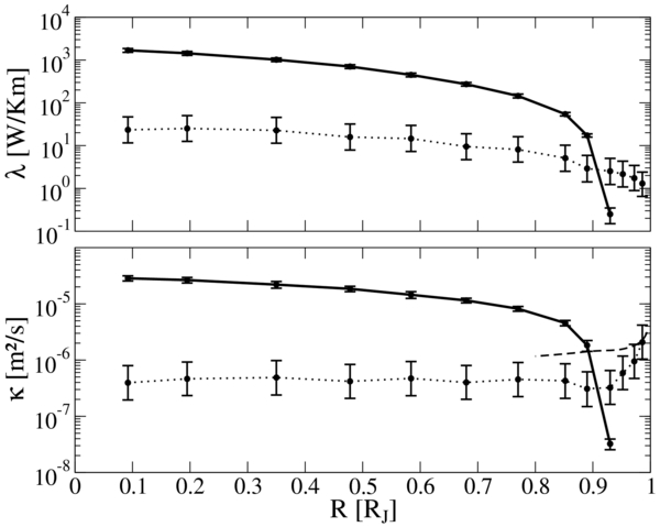
Figure 9. Upper panel: thermal conductivity of the electrons λe derived with the HSE functional (solid line) compared with the ionic contribution λi (dotted line). Lower panel: thermal diffusivity of the electrons κe (solid line) and the respective ionic contribution κi (dotted line). The dashed line is an estimate of Stevenson & Salpeter (1977) for the molecular contribution to the thermal diffusivity.
Download figure:
Standard image High-resolution imageThe electronic contribution behaves very similarly to the electrical conductivity shown in Figure 8. It decreases strongly at the transition from the metallic to the molecular fluid. The Wiedemann–Franz law is fulfilled in the metallic regime, while strong deviations occur in the transition and molecular regime, similar to what was found in an earlier work for pure hydrogen (Holst et al. 2011).
The ionic contribution λi shows a rather small variation with the radius but decreases steadily. At a radius of 0.9 RJ, where electrons become increasingly localized at the nuclei, the ionic contribution becomes dominant. Because of the approximations made in the calculations of λi its error was generally set to be a factor of two.
A similar picture can be drawn for the thermal diffusivity since it behaves correspondingly to the thermal conductivity. The only qualitative difference is that κi rises in the very outer parts of the planet. There it approaches an early estimation of Stevenson & Salpeter (1977) for the molecular contribution of a gaseous H–He mixture.
The numerical values for λ = λe + λi and κ = κe + κi are given in Table 2. The total thermal diffusivity κ never drops below 10−7 m2 s−1.
6.4. Diffusion Coefficients
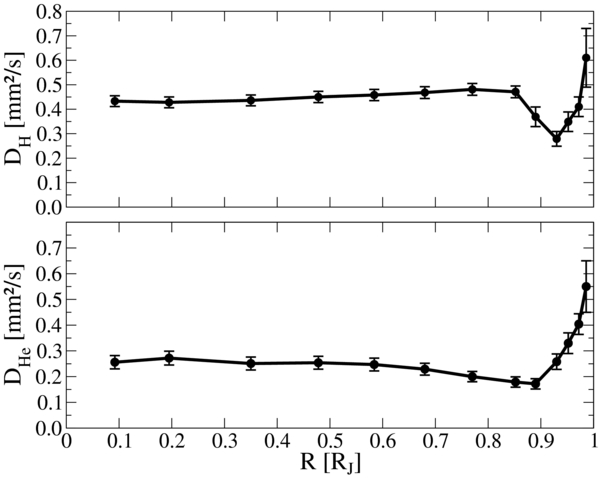
The self-diffusion coefficients for the hydrogen DH and helium DHe nuclei are displayed in Figure 10. In the metallic interior, the diffusion coefficient of hydrogen is about twice as high as the diffusion coefficient of helium, and both show relatively small variations with the radius. This behavior changes drastically as the formation of hydrogen molecules sets in near 0.9 RJ. This process is accompanied with an increase in the scattering cross sections of hydrogen and leads to a drop of DH to the same values as DHe. Outside this transition area, both diffusion coefficients rise systematically due to a decreasing density of the H–He mixture.
Figure 10. Self-diffusion coefficients of hydrogen (upper panel) and helium (lower panel) inside Jupiter.
Download figure:
Standard image High-resolution image
The overall behavior of the diffusion coefficients is consistent with the results for the electrical and thermal conductivities, which are likewise governed by the metal-to-nonmetal transition in the material. Table 2 contains the numerical values for DH and DHe.
7. CONCLUSIONS
In summary, we have applied ab initio simulations to calculate thermodynamic and transport properties along Jupiter's adiabat. These data cover a range of 0.1–0.98 Jupiter radii and are consistent with recent Jupiter models based on the same method and that fulfill the observational constraints (Nettelmann et al. 2012). The data given here can stimulate the development of interior as well as dynamo models that require realistic thermodynamic and transport properties.
For instance, they can be used in magnetohydrodynamic simulations to understand the origin of Jupiter's magnetic field, albeit it is clear that such dynamo simulations will not be able to directly employ all of the results given here without rescaling them first. The reasons for this are of a computational nature, mostly because small-scale turbulence which has its origin, e.g., in small Ekman and Roberts numbers, cannot be completely resolved with the power of today's supercomputers. However, the data presented here can serve as a foothold in the common practice of rescaling the linear into their respective turbulent transport properties (Rüdiger & Hollerbach 2004; Wicht & Tilgner 2010), now allowing one to keep well-founded relative dependencies of the dimensionless numbers with the radius (Gómez-Pérez et al. 2010).
Numerical models for the dynamics in the nonmetallic outer part and in the dynamo region typically assume that heat capacities, the thermal expansion coefficient, and diffusivities are independent of depth (Jones et al. 2011). Our results suggest that this assumption is roughly satisfied in the deep metallic interior. However, the decrease in the electrical conductivity by one order of magnitude inside the metallic regime might already be relevant for dynamo models. Beyond that, the huge radial gradients in the molecular region will have a pronounced impact on the dynamics. Possible implications concern the zone where convection sets in first and remains most vigorous but also the depth of the observed zonal winds (Liu et al. 2008).
Lastly, while standard giant planet models assume an adiabatic, convective interior, the high thermal diffusivity together with a possible presence of a compositional gradient might suppress large-scale convection (Chabrier & Baraffe 2007; Leconte & Chabrier 2012). Such a scenario would have important implications for Jupiter's temperature profile and for core-erosion processes (Wilson & Militzer 2012). Our results can aid future investigations of such problems.
We thank S. Stellmach and B. Holst for inspiring and fruitful discussions and the referee for reviewing the manuscript. This work was supported by the Deutsche Forschungsgemeinschaft (DFG) within the SFB 652 and the SPP 1488. The calculations were performed at the North-German Supercomputing Alliance (HLRN) facilities and at the IT and Media Center of the University of Rostock.