CO (3 − 2) HIGH-RESOLUTION SURVEY OF THE GALACTIC PLANE: R1

J. T. Dempsey; H. S. Thomas; M. J. Currie

doi:10.1088/0067-0049/209/1/8

1. INTRODUCTION

The molecular component of the Galactic plane can be traced by the rotational transitions of carbon monoxide. As the second most abundant molecule, CO is ubiquitous throughout the Galactic plane and is used to trace molecular hydrogen, which as a homonuclear molecule does not emit significantly at low energies. The various rotational transitions of CO are routinely used as a tracer of star formation and have provided detailed information on the velocity structure and morphology of molecular clouds. Molecular clouds provide the reservoir of material for all star formation in the Galaxy. They can be identified as discrete clumps in l − b − v space and lie preferentially along the spiral arms (Stark & Lee 2006).

Large-scale CO surveys of the Galactic plane have proved vital to the study of star formation by identifying molecular clouds and the star-forming clumps within them. Surveys allow the comparison of a range of different environments and these large spectral datasets also reveal valuable information about the large-scale structure of the Galaxy through the identification of spiral arms. CO surveys of the Galactic plane have been carried out for a number of decades (Scoville & Solomon 1975; Sanders et al. 1986) and remain important today. Through the work of Dame et al. (2001) and Dame & Thaddeus (2004), we now have a complete picture of the distribution of ¹²CO (J = 1 → 0) out to latitudes of |b| = 35° although the resolution is low, with a beamwidth of 8.5 arcmin.

A number of targeted surveys have increased the resolution of certain regions. The Galactic Ring Survey (Jackson et al. 2006) observed a region from l =18° to 55 fdg 7 in ¹³CO (J = 1 → 0) at a FHWM of 45 arcsec, while the outer region of the Galactic plane was targeted by a Five-College Radio Astronomy Observatory survey at ¹²CO (J = 1 → 0) by Heyer et al. (1998). The Galactic Center has been observed at ¹²CO (J = 1 → 0) by Bitran et al. (1997), and more recently at ¹²CO (J = 1 → 0) and ¹³CO (J = 1 → 0) using the Nobeyama Radio Observatory (Oka et al. 1998) and at ¹²CO (J = 3 → 2) using the Atacama Submillimeter-wave Telescope Experiment (Oka et al. 2007).

In more recent years, advances in instrumentation as well as a desire for legacy data have led to an increase in the number of large-scale surveys of the Galactic plane. A number of continuum surveys covering a range of wavelengths have been undertaken of the first and fourth quadrants of the Galactic plane. Most notable among these are the Hi-GAL survey (Herschel Infrared Galactic Plane survey; Molinari et al. 2010), and the GLIMPSE I (Galactic Legacy Infrared Mid-Plane survey Extraordinaire; Benjamin et al. 2003) and MIPSGAL (Carey et al. 2009) surveys from Spitzer. In addition to these surveys, there are also the ground-based 1.1 mm Bolocam Northern Galactic Plane Survey (Ginsburg et al. 2013; Aguirre et al. 2011), the ATLASGAL survey at 870 μm (Contreras et al. 2013), the CORNISH survey of UCHII regions (Purcell et al. 2008), and UKIDSS (UK IR Deep Sky Survey; Lawrence et al. 2007), which will trace more evolved sources. Another important survey currently in progress is the JPS (JCMT Galactic Plane Survey; Moore et al. 2005) which will map regions of the plane with a resolution of 14 arcsec at 850 μm and 8 arcsec at 450 μm.

This paper outlines the first release of data from the CO High Resolution Survey (COHRS) of first quadrant of the Galactic plane—the latest contribution to the survey collection. One of main aims of COHRS is to complement existing datasets; to maximize this potential, the region was selected to ensure the greatest overlap with current and upcoming surveys.

For COHRS we have mapped the region in ¹²CO (J = 3 → 2). This transition is less optically thick than the J = 1 → 0 and J = 2 → 1 transitions and its higher frequency allows for higher-resolution data than previously surveyed at these longitudes. With the J = 3 level at 33 K above ground and a critical density of ∼5 × 10⁴ cm⁻³, this transition is an excellent tracer of molecular clouds and particularly of the warm material (10–50 K) of medium density (10⁴ cm⁻³ at 20 K) around cores heated by active star formation. CO (J = 3 → 2) is also a useful tracer of outflow activity, a classic indicator of the very early stages of star formation. (Banerjee & Pudritz 2006).

This transition was also chosen for its abundance and distribution in the Galactic plane. Its higher critical density means it has a more compact distribution than the lower CO transitions which, in practical terms, allows a substantial region of the plane to be mapped in a reasonable number of hours. Meanwhile its relatively high abundance and the position of the J = 3 → 2 transition in the atmospheric transmission window means good-quality data can be taken in less than perfect weather conditions. These are all vital considerations for an over-subscribed telescope.

The optical depth of CO (J = 3 → 2) is likely to be high toward the more massive cloud complexes and will certainly be optically thick toward the center of dense cores (Polychroni et al. 2012). Nevertheless CO (J = 3 → 2) remains an excellent tracer of the more diffuse, transitional material between cores.

In this paper we describe the data-acquisition strategy and data-reduction procedure for COHRS in Section 2. In Section 3 we provide information about where to access these data online, then go on to discuss the noise characteristics and reduction artifacts in Section 4. We present the results in the form of integrated intensity maps and longitude-velocity diagrams in Section 5, followed by a discussion of future work in Section 6. A full analysis of the data will be presented in a future paper.

2. OBSERVATIONS AND DATA REDUCTION

This survey covers |b| ⩽ 0 fdg 5 between 10° < l < 65°, with the data presented in this first release paper covering the region |b| ⩽ 0 fdg 5 between 10 fdg 25 < l < 17 fdg 5 and 50 fdg 25 < l < 55 fdg 25, and |b| ⩽ 0 fdg 25 between 17 fdg 5 < l < 50 fdg 25. A couple of additional regions are extended to the full latitude range; see Table 1 for details. The COHRS region was chosen to coincide with the area covered by a number of important surveys, notably GLIMPSE (|l| = 10° to 65°, |b| ⩽ 1), Bolocam (−10 fdg 5 < l < 90 fdg 5, |b| ⩽ 0 fdg 5), JPS (sub-regions between 8° < l < 62°, |b| ⩽ 2°), and Hi-GAL (−60° < l < 60°, |b| ⩽ 1°).

Table 1. COHRS Summary (Release 1)

Survey Coverage
−05 < b< +05	+10° < l < +175
"	+4525 < l < +4575
"	+4825 < l < +4875
"	+5025 < l < +5525
−05 < b < +025	+175 < l < +19°
−025 < b < +025	+19° < l < +4525
"	+4575 < l < +4825
"	+4875 < l < +5025
Survey Parameters
Molecule	¹²CO (J = 3 → 2)
Angular resolution^a	138/166
Velocity range	−30 km s⁻¹ to +155 km s⁻¹
Velocity resolution^a	0.42 km s⁻¹/1 km s⁻¹
Tsys range	290 to 1200 K (mean = 610 K)
Approximate rms^a,b	2 K/1 K
Angular sampling	6''
Survey area	29 deg²

Notes. ^aRaw values/smoothed values. ^bSee Table 3 for mean rms per tile.

Download table as: ASCII Typeset image

2.1. Data Acquisition

CO (J = 3 → 2) (345.786 GHz) observations were carried out with the Heterodyne Array Receiver Program (HARP; Buckle et al. 2009) on the James Clerk Maxwell Telescope (JCMT) in Hawaii. The area covered by this survey totals 29 square degrees and is summarized in Table 1.

HARP consists of 16 superconductor–insulator–superconductor (SIS) heterodyne detectors arranged in a 4 × 4 grid and separated by 30 arcsec. At this frequency, HARP has a resolution of 14 arcsec and a main-beam efficiency of η_mb = 0.61.

The Auto-Correlation Spectral Imaging System (ACSIS; Buckle et al. 2009) back-end was set up with a 1 GHz bandwidth giving a frequency resolution of 0.488 MHz or a velocity resolution of 0.42 km s⁻¹. The sampling rate was 0.1 s which is the fastest mapping speed of which ACSIS is capable. This enabled a data cube of 0 fdg 5 × 0 fdg 5 to be completed in less than an hour. The bandwidth (−400 km s⁻¹<v_LSR < +400 km s⁻¹) was selected to be wide enough to include all the emission at the extremes of the velocity range seen toward the inner region of the Galactic plane while still leaving sufficient baseline for subtraction and noise determination. The final data cubes in the release have been cropped to a velocity range of −30 km s⁻¹<v_LSR < +155 km s⁻¹.

Each tile was observed in position-switched raster (on-the-fly) mode with 1/2 array spacing. In this configuration the array is stepped by half its width perpendicular to the scan direction before each new row is started. This results in spectra separated by 7.3 arcsec perpendicular to the scan direction. It also provides enhanced uniformity of the noise with redundancy against poorly performing or dead receptors. This redundancy is further promoted by the use of the basket-weave technique whereby each tile is observed twice with the array oriented in perpendicular scan directions.

The off-position was selected as +2 fdg 5 above the Galactic plane. This was chosen to be far enough away as to be free from contaminating emission. However, a few tiles do contain emission in their off position which presents as a negative spectral feature in the reduced dataset. Nearly all of the emission in the off positions is local, however, with zero velocity. As such it does not interfere with the dynamics of the survey data.

As standard procedure at the JCMT, the pointing is checked every 1–1.5 hr or between any large slew in azimuth or elevation. The nominal pointing performance of the HARP on JCMT is ∼1 farcs 5–2 farcs 5 rms in azimuth and fractionally more in elevation. These numbers are higher than the other instruments on the JCMT due to slight misalignments of the HARP K-mirror. A check of the pointing on the nights in questions reveals our pointing to be around ∼2''–2 farcs 5 rms. We lie at the upper end of pointing performance due to the high opacity in which many of the observations were carried out. Irrespective of the pointing residuals, once the telescope is on a source the tracking accuracy is sub-arcsecond for the duration of a typical observation.

The data were observed as a mixture of PI time, Directors Discretionary Time (DDT), empty-queue or poor-weather backup time. The PI time covered three semesters from 2010 to 2012 and was assigned an opacity range of 0.12 <τ₂₂₅ < 0.25. The data collected during DDT and empty queue time were observed in opacities ranging from τ₂₂₅ ∼ 0.05 through to τ₂₂₅ ∼ 0.3. This has resulted in non-uniform sensitivity across the completed map. As a guideline, we typically achieve a mean $T_{\rm {A}}^*$ rms in the initial reduced data of ∼2 K. After rebinning to a velocity resolution of 1 km s⁻¹ this improves to ∼1 K.

2.2. Data Processing

The data were processed using the ORAC-DR pipeline (Cavanagh et al. 2008) narrowline recipe, which employs tasks from Starlink¹ packages KAPPA (Currie et al. 2008), SMURF (Jenness et al. 2008), and CUPID (Berry et al. 2007) to generate reduced cubes. It used the Kapuahi release of the software.

The recipe has two broad phases: quality assurance (QA) and iterative creation of the spectral cube and other products.

The QA phase begins by masking defective spectra in three stages. The first two stages flag small time chunks of data where an individual receptor becomes temporarily noisy or exhibits non-linear baselines compared with the bulk of its spectra. The next filter masks entire receptors with non-linear baselines. This filtering reduces the sensitivity to some degree but this was deemed an acceptable trade off for more uniform maps with minimal striping. For the final step, various QA criteria are tested based upon a set of pre-defined parameters. We elected to use the default QA parameters associated with the ACSIS ORAC-DR pipeline. These are given in Table 2. Next the pipeline applies thresholds to remove any spikes, and trims the noisy edge regions.

Table 2. Quality Assurance Parameters in the ACSIS ORAC-DR Pipeline

Parameter^a (X)	Value	Description
BADPIX_MAP	0.3	Maximum number of bad pixels allowed in the final map
GOODRECEP	10	Minimum number of working receptors
TSYSBAD	2000	Upper limit of T_sys for raw time-series data
FLAGTSYSBAD	0.5	Flag as bad any receptor with X% of data points with T_sys>Tsysbad
TSYSMAX	1500	Median T_sys/receptor after flagging by FLAGTSYSBAD must be <X
TSYSVAR	1.0	X% is the maximum variation in T_sys between receptors
RMSVAR_RCP	1.0	Maximum variation (%) in rms noise between receptors
RMSVAR_SPEC	0.4	Maximum variation (%) in rms noise across full spectrum
RMSVAR_MAP	2.0	Maximum variation (%) in rms noise from one map pixel to another
RMSTSYSTOL	0.5	Measured rms must not differ from rms calculated from the T_sys by >X%
RMSTSYSTOL_QUEST	0.15	Limit to mark data questionable
RMSTSYSTOL_FAIL	0.2	Limit to mark data failed
RMSMEANTSYSTOL	1.0	Data with an rms >X% of the mean rms will get masked out
CALPEAKTOL	0.2	Calibrators must agree with their expected peak values within X%
CALINTTOL	0.2	Calibrators must agree with their expected integrated values within X%
RESTOL	1	Average residuals following baseline subtraction should be <Xσ
RESTOL_SM	1	Average residuals no larger than Xσ over any four adjacent channels

Note. ^aFor a more detailed description of these parameters, see Hatchell (2008).

Download table as: ASCII Typeset image

Then the iterative phase begins. The recipe converts and combines the raw time-series spectra into a composite data cube with (l, b, v) axes. In ORAC-DR parlance it is called the group cube. The combination of observations leads to a better definition of the regions of emission, and hence more accurate baseline subtraction.

The initial baseline procedure creates an approximate mask of the emission from the group cube. The mask is made by smoothing the spectra with a top-hat filter of width five pixels along the spatial axes and ten pixels along the spectral axis, condensing each spectrum to 32 bins to further improve the signal-to-noise ratio, and then applying a progressive iterative sigma clipping. The mask is then applied to the individual observations, and new baseline fits are found for each spectrum without any smoothing or binning.

During each iteration, maps of various moments can be created by collapsing the baseline-subtracted group cube. Although we are not releasing any of these, an important by-product of this step is an improved emission mask for the next iteration. The recipe applies the CUPID FINDCLUMPS task to the smoothed cube to identify clumps of emission invoking its version of ClumpFind based on the algorithm presented in Williams et al. (1994). FINDCLUMPS generates a 3σ emission mask of clumps comprising at least 50 pixels.

The recipe then regenerates time-series spectra for each observation after application of the emission mask, and new baselines are fitted and subtracted. These improved time-series data are then used to remake the group spatial-frequency data cube. In practice only one iteration was needed.

For the final products, the data were then regridded to 6 arcsec pixels and convolved with a 9 arcsec Gaussian beam; this degraded our resolution to 16.6 arcsec in the final map. Along the spectral axis, the data were rebinned to 1 km s⁻¹ per pixel scale. A paper is in preparation describing the ORAC-DR heterodyne pipeline in detail.

3. DATA RELEASE

The COHRS data presented in this paper are available online from the CANFAR data archive.² In this first release we offer 90 tiles in FITS format with half a degree width in longitude (± 0.25 deg from the central longitude position). The latitude range will vary depending on the data collected to date. Each tile follows a naming convention reflecting its central longitude and latitude; this is then appended by a suffix depending on the nature of the file. The different types of files available are shown in the list below; their suffixes are given in square brackets. Table 3 gives the base name, the mean opacity, and the mean rms for each tile. All intensities in the release are in units of $T_{\rm {A}}^*$ . To convert the antenna temperatures $T_{\rm {A}}^*$ to main beam brightness temperatures, T_MB, they can be divided by the main beam efficiency, η_mb = 0.61, determined from observations of planets (Buckle et al. 2009). The uncertainty in η_mbis approximately 10%–15%.

Table 3. COHRS Tiles Summary

Tile Name^a	τ₂₂₅^b	rms^c
Tile Name^a	τ₂₂₅^b	(K)
COHRS_10p50_0p00^d	0.073	0.49
COHRS_11p00_0p00^d	0.190	1.10
COHRS_11p50_0p00^d	0.052	0.48
COHRS_12p00_0p00^d	0.092	0.55
COHRS_12p50_0p00^d	0.153	0.78
COHRS_13p00_0p00^d	0.206	0.68
COHRS_13p50_0p00^d	0.151	0.97
COHRS_14p00_0p00^d	0.070	0.54
COHRS_14p50_0p00^d	0.133	0.72
COHRS_15p00_0p00^d	0.184	0.49
COHRS_15p50_0p00^d	0.225	0.74
COHRS_16p00_0p00^d	0.204	0.55
COHRS_16p50_0p00^d	0.079	0.57
COHRS_17p00_0p00^d	0.253	0.83
COHRS_17p50_0p00	0.223	1.60
COHRS_18p00_0p00	0.230	1.28
COHRS_18p50_0p00	0.210	0.98
COHRS_19p00_0p00	0.212	1.17
COHRS_19p50_0p00	0.105	0.69
COHRS_20p00_0p00	0.149	0.65
COHRS_20p50_0p00	0.137	0.63
COHRS_21p00_0p00	0.233	1.52
COHRS_21p50_0p00	0.179	1.24
COHRS_22p00_0p00	0.169	1.21
COHRS_22p50_0p00	0.229	1.44
COHRS_23p00_0p00	0.246	1.08
COHRS_23p50_0p00	0.201	1.07
COHRS_24p00_0p00	0.205	1.31
COHRS_24p50_0p00	0.182	1.15
COHRS_25p00_0p00	0.199	1.40
COHRS_25p50_0p00	0.188	1.05
COHRS_26p00_0p00	0.182	0.99
COHRS_26p50_0p00	0.187	1.02
COHRS_27p00_0p00	0.159	1.37
COHRS_27p50_0p00	0.198	0.74
COHRS_28p00_0p00	0.127	0.49
COHRS_28p50_0p00	0.122	0.50
COHRS_29p00_0p00	0.216	0.52
COHRS_29p50_0p00	0.227	0.57
COHRS_30p00_0p00	0.207	1.22
COHRS_30p50_0p00	0.230	0.75
COHRS_31p00_0p00	0.246	1.19
COHRS_31p50_0p00	0.230	0.74
COHRS_32p00_0p00	0.245	1.17
COHRS_32p50_0p00	0.212	1.07
COHRS_33p00_0p00	0.136	0.73
COHRS_33p50_0p00	0.272	0.69
COHRS_34p00_0p00	0.205	0.72
COHRS_34p50_0p00	0.182	0.93
COHRS_35p00_0p00	0.175	0.63
COHRS_35p50_0p00	0.172	0.71
COHRS_36p00_0p00	0.204	0.93
COHRS_36p50_0p00	0.174	1.07
COHRS_37p00_0p00	0.196	0.96
COHRS_37p50_0p00	0.183	0.63
COHRS_38p00_0p00	0.208	1.08
COHRS_38p50_0p00	0.270	0.78
COHRS_39p00_0p00	0.258	1.38
COHRS_39p50_0p00	0.301	1.42
COHRS_40p00_0p00	0.258	1.11
COHRS_40p50_0p00	0.183	1.03
COHRS_41p00_0p00	0.211	0.94
COHRS_41p50_0p00	0.252	0.98
COHRS_42p00_0p00	0.171	1.32
COHRS_42p50_0p00	0.174	0.88
COHRS_43p00_0p00	0.198	1.07
COHRS_43p50_0p00^d	0.072	0.44
COHRS_44p00_0p00	0.070	0.49
COHRS_44p50_0p00	0.085	0.53
COHRS_45p00_0p00	0.110	0.57
COHRS_45p50_0p00^d	0.197	0.94
COHRS_46p00_0p00	0.092	0.60
COHRS_46p50_0p00	0.132	0.54
COHRS_47p00_0p00	0.121	0.59
COHRS_47p50_0p00	0.185	0.65
COHRS_48p00_0p00	0.133	0.70
COHRS_48p50_0p00^d	0.216	0.94
COHRS_49p00_0p00	0.117	0.69
COHRS_49p50_0p00	0.064	0.45
COHRS_50p00_0p00	0.119	0.75
COHRS_50p50_0p00^d	0.166	0.90
COHRS_51p00_0p00	0.163	0.87
COHRS_51p50_0p00^d	0.147	0.85
COHRS_53p00_0p00	0.147	0.79
COHRS_53p50_0p00^d	0.251	1.43
COHRS_54p00_0p00^d	0.187	0.85
COHRS_54p50_0p00^d	0.191	1.01
COHRS_55p00_0p00^d	0.129	0.85

Notes. ^aIn the archive this name is appended by text describing the map type (integrated, cube or l − v). The numbers in the name give the central longitude and latitude of the tile. ^bThe mean 225-GHz opacity taken from the Caltech Submillimeter Observatory (CSO) tau dipper. ^cThe mean $T_{\rm {A}}^*$ rms in the tiles rebinned to 1 km s⁻¹ channel width. ^dTiles with full extent to |b| ⩽ 0 fdg 5.

Download table as: ASCIITypeset images: 1 2

The following products are available online.

1.
The reduced cubes in units of $T_{\rm {A}}^*$ re-binned to 1 km s⁻¹ channel width [CUBE_REBIN].
2.
Integrated intensity maps collapsed over all emission above 3σ [INTEG].
3.
Position–velocity maps collapsed over all emission above 3σ [LV].

Raw data can be obtained from the JCMT Science Archive at CADC (following the expiration of the proprietary period) or by contacting the authors directly.

4. NOISE CHARACTERIZATION

The first COHRS data release set contains 24.45 megapixels, and a total of 3.15 gigavoxels. Figure 1 shows a histogram of the antenna temperature for all voxels, or (l, b, v) positions, in the survey. The main plot shows the distribution on a logarithmic scale while the inset shows a linear scale with a Gaussian fit overlaid. The Gaussian has an FWHM of 0.94 K. The distribution displays a strong positive tail due to the contribution from the ¹²CO emission. Also evident is a weak negative tail likely due to contributions from those tiles with emission in the reference position. This was investigated further by inverting each data cube and running the CUPID FINDCLUMPS task as described in Section 2.2. Table 4 lists those tiles that showed strong (3σ) and weak (2σ) negative emission and the velocities at which these features are found. Observations of the reference positions for these tiles are currently underway and will be provided in the next data release.

Table 4. COHRS Tiles with Off-position Contamination

Tile Name	3σ^a	2σ^b
Tile Name	(km s⁻¹)	(km s⁻¹)
COHRS_14p00_0p00	⋅⋅⋅	21
COHRS_15p50_0p00	17	17
COHRS_16p50_0p00	34	34
COHRS_17p50_0p00	⋅⋅⋅	7–10
COHRS_18p50_0p00	⋅⋅⋅	25–26
COHRS_22p50_0p00	⋅⋅⋅	7–9
COHRS_23p00_0p00	7–9	7–9
COHRS_23p50_0p00	⋅⋅⋅	7–9
COHRS_24p00_0p00	⋅⋅⋅	7–9
COHRS_26p00_0p00	⋅⋅⋅	7–9
COHRS_26p50_0p00	⋅⋅⋅	7–9
COHRS_27p50_0p00	⋅⋅⋅	4–8
COHRS_28p00_0p00	5	4–6, 33
COHRS_28p50_0p00	6–7	4–7
COHRS_29p00_0p00	⋅⋅⋅	4–6
COHRS_29p50_0p00	⋅⋅⋅	5
COHRS_30p00_0p00	7–9	6–10
COHRS_30p50_0p00	6–9	6–9
COHRS_31p50_0p00	⋅⋅⋅	6–8
COHRS_32p50_0p00	⋅⋅⋅	6–8
COHRS_34p50_0p00	⋅⋅⋅	19–21
COHRS_37p00_0p00	⋅⋅⋅	73
COHRS_39p00_0p00	⋅⋅⋅	25–27
COHRS_40p50_0p00	⋅⋅⋅	27, 31, 35
COHRS_41p50_0p00	⋅⋅⋅	7.0
COHRS_53p50_0p00	⋅⋅⋅	10.0

Notes. ^aRadial velocities in km s⁻¹ at which 3σ detections of negative features are present. ^bRadial velocities in km s⁻¹ at which 2σ detections of negative features are present.

Download table as: ASCII Typeset image

Figure 2 shows a histogram of the noise in each pixel of the survey. These values are determined from taking the standard deviation of baseline regions of each spectrum between −150 km s⁻¹<v_lsr < −100 km s⁻¹ and +200 km s⁻¹<v_lsr < +250 km s⁻¹. This histogram peaks around 0.5 K but the tail highlights the spread of the noise across the survey. This inset also shows the data on a linear scale where multiple peaks can be seen. These peaks reflect the wide range of observing conditions in which these tiles were taken. The noisiest tiles, responsible for the peak around 1 K, are typically the result of observing in poor weather or at low elevations. A further factor contributing to high noise is the integration time per pixel. This is dependent on the number of HARP receptors included in the reduction. A low integration time may be the result of dead receptors on the instrument (which has varied over the duration of this survey), or entire receptors (or time slices) that were later excluded by the reduction software.

The mean rms for each re-binned tile is given in Table 3. This value is a mean of all the pixel values calculated for Figure 2. In some cases the final tiles include maps observed on different nights and in different conditions resulting in mean rms values that are not representative of the individual maps. The spatial noise distribution across the survey, and within each tile, can be best visualized in Figure 3, a two-dimensional map of the noise temperature. This is useful for highlighting the relative quality of the individual maps that contribute to each tile.

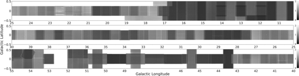
**Figure 3.** Two-dimensional map of the $T_A^*$ noise distribution for COHRS in unit of K. The noise temperature in each pixel was determined by collapsing each spectrum between −150 km s⁻¹<v_lsr < −100 km s⁻¹ and +200 km s⁻¹<v_lsr < +250 km s⁻¹. The wide scale reflects the range of observing conditions.
Download figure:
Standard image High-resolution image

**Figure 3.** Two-dimensional map of the $T_A^*$ noise distribution for COHRS in unit of K. The noise temperature in each pixel was determined by collapsing each spectrum between −150 km s⁻¹<v_lsr < −100 km s⁻¹ and +200 km s⁻¹<v_lsr < +250 km s⁻¹. The wide scale reflects the range of observing conditions.
Download figure:
Standard image High-resolution image

Some regions are seen to display a faint residual tartan pattern (for example between l = 17° and l = 18° in Figure 4). This is one of the effects of the non-uniformity of the integration time due to missing or rejected receptors with the characteristic pattern arising from the basket-weaved observing mode. The reductions did not account for receptor-to-receptor sensitivities. Flat-fielding and Fourier-transform-based destriping reduction methods, which we expect to minimize this artifact, are in development. A second data release will include both new data collected in the interim and an improved reduction of the data presented in this paper (H. S. Thomas et al. in preparation).

5. RESULTS

5.1. Integrated Intensity

Figure 4 shows the integrated intensity (or zeroth moment) map for COHRS. This is produced by collapsing over all clumps in the reduced cube that have been identified with ClumpFind as being 3σ or greater.

There is considerable faint, extended emission detected. This is somewhat surprising as the critical density of CO (J = 3 → 2) (∼10⁴ at 20 K) suggests we might expect to see emission concentrated in dense clumps of star-forming regions connected by tight filamentary structures. This is the morphology of emission commonly seen in submillimeter maps or with the high-density tracer CS (J = 2 → 1), which has a similar critical density. A higher than expected level of extended emission may be the result of high optical depth in CO (J = 3 → 2). This can result in photon trapping which effectively reduces the critical density allowing lower density material to be traced (Scoville & Solomon 1974).

The l − v diagrams shown in the next section (Figure 6) show a wide range of velocities and it is likely when looking at integrated emission maps that we are seeing multiple clouds along the line of sight superimposed on each other.

Well-studied regions such as W49 and W43 show highly peaked emission with a detailed velocity structure. While star-forming region such as these dominate the emission, the high resolution of COHRS reveals delicate structures and peaked cores on even the smallest scales.

5.2. Longitude–Velocity

A longitude–velocity (l − v) map for the full COHRS region is shown in Figure 5. We also show the diagram in greater detail in Figure 6. These maps are made by collapsing the re-binned cubes over the full latitude range available at each longitude. As expected, this correlates closely with the ¹³CO l − v maps from the Galactic Ring survey (Figure 3. of Jackson et al. 2006). Most of the emission is concentrated in this "molecular ring", which lies in the area between 3–5 kpc from the Galactic Center and corresponds to a longitude range of ∼22° < l < 32° in Figure 5. The molecular ring includes the origins of four spiral arms. Although initially believed to be a true ring-like structure, Vallee (2008) has collected considerable evidence to support the idea that this ring is, in fact, an artifact of observing these spiral arms at low resolution (Englmaier & Gerhard 1999; Nakanishi & Sofue 2006) and the ring-like structure arises as a result of overlapping or twisting of the spiral arms (Dobbs & Burket 2012).

In our inner region from 10° < l < 20° the models shown in Figure 3 of Vallee (2008) predict eight components distinct in velocity. These components are actually the four known spiral arms displaying multiple velocity components along the line of sight. The Perseus arm in particular has three velocity ranges in this longitude region. The benefits of high resolution are immediately clear with multiple spiral arms able to be resolved. In the inner region in particular we see many components at high velocity; these are unlikely to be directly related to an arm but are more likely to be high velocity material, a natural product of the energetics seen toward the Galactic Center. Nevertheless we have been able to detect them and they subtend several arcminutes so are clearly extremely large structures.

Figure 6 illustrates the detailed velocity structure of the data where multiple distinct velocity components and structures are evident at all longitudes that do not show up in Figure 5.

6. FOLLOW-UP WORK

COHRS is an ongoing project, with future observations focusing on expanding outward in latitude to fill in the range |b| ⩽ 0 fdg 5. The potential time constraints surrounding the future of the JCMT mean we may be required to prioritize our awarded time. In this situation we will choose to prioritize those regions that overlap with the rescoped JCMT Plane Survey (JPS) which focuses on 4° width strips around 10°, 20°, 30°, 40°, 50°, and 60° longitude. By selecting these regions we not only provide complimentary data to the JPS but, with the same reasoning, will sample different, unbiased, regions of the plane. New data collected will be presented to the community as Release 2 of COHRS. Release 2 will also include a complete reprocessing of all the data with more advanced reduction techniques. We anticipate this new reduction will remove some of the artifacts seen in the data presented here and further minimize the noise distribution.

In addition to describing the reprocessing of the data, the follow-up COHRS paper (H. S. Thomas et al. in preparation) will include a full analysis of the data. The velocity information for example will be vital for investigating the role of turbulence in the star forming process, with models of turbulent fragmentation suggesting a direct link between the power spectrum of the turbulent velocity field and the resulting mass function of the cores that form (Padoan & Nordlund 2002; Klessen et al. 2000).

We will produce a clump catalog using the dual techniques of ClumpFind (Williams et al. 1994) and Fellwalker (Berry et al. 2007); this catalog will allow an initial comparison with existing datasets and the final catalog will be made available online. A number of surveys overlap with the COHRS region and these will allow an investigation of the local conditions for a range of different stages of stellar evolution. Star counts from the GLIMPSE survey give an indication of star formation efficiency rates, while survey data from CORNISH can be used to determine the locations of high-mass young stars. Similarly, UKIDSS, along with GLIMPSE, gives the location of more evolved sources in OB associations. The continuum surveys, ATLASGAL and BGPS (Contreras et al. 2013; Ginsburg et al. 2013), have a strong overlap with COHRS, providing valuable continuum information on the youngest star-forming regions. This will be complemented further by the in-progress JPS survey, which will provide matching resolution and improved sensitivity continuum measurements of the same region.

COHRS is also expected to be a valuable resource for those searching for outflows. The detection of outflows is one of the primary indicators of the current state of star formation within a clump. Traditionally the identification of outflows has relied on a "by eye" technique which is impractical for large volumes of data. However, a number of machine-learning tools are in development to allow the automated detection of outflows for large datasets such as COHRS (Beaumont et al. 2011).

7. SUMMARY

COHRS is mapping the Galactic plane in ¹²CO (J = 3 → 2) using HARP on the JCMT with an angular resolution of 14 arcsec and the data sampled on 6 arcsec pixels. Eventually COHRS will cover |b| ⩽ 0 fdg 5 between 10° < l < 65°. The data presented in this first release paper cover the region |b| ⩽ 0 fdg 5 between 10 fdg 25 < l < 17 fdg 5 and 50 fdg 25 < l < 55 fdg 25, and |b| ⩽ 0 fdg 25 between 17 fdg 5° < l < 50 fdg 25. In total the data presented in this paper cover 29 deg². This is the highest resolution large CO map to date and is available to the community online.

The authors thank Toby Moore and Antonio Chrysostomou for their valuable input and support of the COHRS project.

The James Clerk Maxwell Telescope is operated by the Joint Astronomy Centre on behalf of the Science and Technology Facilities Council of the United Kingdom, the National Research Council of Canada, and (until 2013 March 31) the Netherlands Organisation for Scientific Research.

CO (3 − 2) HIGH-RESOLUTION SURVEY OF THE GALACTIC PLANE: R1

Article metrics

Permissions

Author e-mails

Author affiliations

Dates

ABSTRACT

1. INTRODUCTION