


ABSTRACT
The Columbia University–Universidad de Chile CO Survey of the southern Milky Way is used to separate the CO(1–0) emission of the fourth Galactic quadrant within the solar circle into its dominant components, giant molecular clouds (GMCs). After the subtraction of an axisymmetric model of the CO background emission in the inner southern Galaxy, 92 GMCs are identified, and for 87 of them the twofold distance ambiguity is solved. Their total molecular mass is M(H2) = 1.14 ± 0.05 × 10⁸ M☉, accounting for around 40% of the molecular mass estimated from an axisymmetric analysis of the H2 volume density in the Galactic disk, M(H2)disk = 3.03 × 10⁸ M☉. The large-scale spiral structure in the southern Galaxy, within the solar circle, is traced by the GMCs in our catalog; three spiral arm segments, the Centaurus, Norma, and 3 kpc expanding arm, are analyzed. After fitting a logarithmic spiral arm model to the arms, tangent directions at 310°, 330°, and 338°, respectively, are found, consistent with previous values from the literature. A complete CS(2–1) survey toward IRAS point-like sources with far-IR colors characteristic of ultracompact H ii regions is used to estimate the massive star formation rate per unit H2 mass (MSFR) and the massive star formation efficiency ( ) for GMCs. The average MSFR for GMCs is 0.41 ± 0.06 L☉/M☉, and for the most massive clouds in the Norma arm it is 0.58 ± 0.09 L☉/M☉. Massive star formation efficiencies of GMCs are, on average, 3% of their available molecular mass.
Export citation and abstract BibTeX RIS
1. INTRODUCTION
Within the Galactic disk, at 100 pc scales, the molecular gas is contained mostly in the form of giant molecular clouds (GMCs; Dame et al. 1986; Bronfman et al. 1988b; Williams & McKee 1997). The large-scale clumpy structure of the CO emission in longitude–velocity diagrams is clear evidence of the organization of the gas into these large objects (Bronfman et al. 1989). The principal characteristic of GMCs is the role they play as tracers of the large-scale structure in the Galaxy and as birthplaces of most of the massive stars in the Galactic disk.
As for the origin of GMCs, it is accepted that in the disk of the Milky Way they are formed as the molecular gas enters in the spiral wave pattern of the gravitational potential energy of the Galactic disk (Elmegreen 1994). Tidal shear forces among GMCs are weaker within the spiral arms than for the interarm regions, making the gravitational collapse more feasible (Luna et al. 2006). Other mechanisms, such as the growth by collisions, are apparently too inefficient to reproduce the observed power-law mass distribution of GMCs (Elmegreen 1993; Tan et al. 2013).
GMCs are excellent tracers of large-scale Galactic structure. The best example is found in the Carina spiral arm, traced over 20 kpc in the outer Galaxy by more than 40 GMCs, between l = 270° and l = 330° in Galactic longitude (Grabelsky et al. 1987, 1988). Dame et al. (1986) reconstructed a three-spiral-arm model for the first Galactic quadrant based on their catalog defined in CO and suggested that the containment of the largest molecular clouds in the arms demonstrates that CO emission is enhanced in the arms not only because the clouds are hotter, as suggested by Sanders et al. (1985), but also mainly because they are larger and contain more mass.
GMCs are the known places of massive star formation. Massive stars (M > 8 M☉) originate mainly inside dense, compact clumps (ultracompact (UC) H ii regions) in giant molecular clouds (Evans 1999; Mac Low & Klessen 2004; Krumholz & McKee 2005; Tan 2005; Luna et al. 2006; McKee & Ostriker 2007; Zinnecker & Yorke 2007; Schuller et al. 2010). At large scales, Bronfman et al. (2000) showed that the radial distribution of massive-star-forming regions follows, on average, that of the molecular gas in the inner Galactic disk for all galactocentric radii and that the massive star formation is highest at the peak of the southern "molecular ring" (understood as an azimuthally averaged molecular gas distribution of the Galactic disk), ranging 0.5 ⩽ R/R☉ ⩽ 0.6 in the galactocentric radius. For the fourth Galactic quadrant (IVQ), Luna et al. (2006) showed that massive star formation occurs in regions with high molecular gas density, roughly coincident with the line of sight tangent to spiral arms. At smaller scales, giant molecular clouds harbor most of the massive star formation in the Galaxy (Luna et al. 2006; Mac Low & Klessen 2004; McKee & Ostriker 2007; Zinnecker & Yorke 2007). An example of this is the extremely high velocity molecular outflow, a signature of massive star formation (Krumholz 2006, and references therein), in the G331 region (Bronfman et al. 2008; Merello et al. 2013).
While extensive work has been carried out to identify and find the physical characteristics and spatial distributions of GMCs in the first Galactic quadrant (IQ) within the solar circle (Dame et al. 1986; Scoville et al. 1987; Solomon et al. 1987), no equivalent catalog of GMCs in the IVQ within the solar circle has been published yet. For the IQ, different methods have been used to define the GMCs: topologically closed surfaces in the three-dimensional LBV (longitude, latitude, velocity) CO data phase space (Scoville et al. 1987; Solomon et al. 1987), "clipping" the CO data below a certain temperature threshold (Myers et al. 1986), and subtraction from the observed CO emission of a synthetic data set generated from an axisymmetric model of the Galactic molecular gas distribution (background subtraction; Dame et al. 1986) to "extract" the GMCs from the complex CO background emission in which they are immersed. In this work, we use the CO data set from the Columbia University–Universidad de Chile Southern CO Survey of the Milky Way (Bronfman et al. 1989; hereinafter referred to as CO Survey) to define GMCs in the three-dimensional phase space through the subtraction, from the CO data, of an axisymmetric model (ASM; Bronfman et al. 1988b) of the complex CO background emission following Dame et al. (1986).
We estimate the massive star formation rate and massive star formation efficiency of GMCs in our catalog by taking advantage of a complete CS(2–1) survey toward IRAS point-like sources with far-IR (FIR) colors characteristic of UC H ii regions (Bronfman et al. 1996) complemented by a new unpublished CS(2–1) survey (L. Bronfman et al. 2014, in preparation). Hereinafter we refer to the whole CS(2–1) data set as the CS(2–1) survey and to the IRAS point-like UC H ii regions as IRAS/CS sources. We select massive-star-forming regions from the IRAS point source catalog because most of the embedded massive star luminosity is emitted around 100 μm in the mid- and far-IR (see Figure 2 in Faúndez et al. 2004). The IRAS point sources are selected by their FIR colors, using the Wood & Churchwell (1989) criterion for UC H ii regions, which traces well the population of young embedded massive stars (Faúndez et al. 2004) emitting also in the millimeter continuum. This continuum survey shows that massive cold cores, the very early stages of MSF, are associated with the central UC H ii region. The CS(2–1) emission is a great tracer in that it is only excited in regions of densities greater than 104–105 cm−3. We detected the line emission for about 75% of the candidates. This is a complete sample of the most massive and luminous regions of massive star formation in the Galaxy. There are more recent Galactic surveys in the mid-IR and submillimeter regions of the spectrum (GLIMPSE, MIPSGAL, and ATLASGAL), but (1) there are no complete line surveys to determine their kinematic information, and (2) only a small fraction of the luminosity from massive-star-forming regions comes in the near-IR (NIR) and submillimeter wavelengths (Faúndez et al. 2004; Tanti et al. 2012).
In Section 2 we present for the first time a complete catalog of molecular clouds in the IVQ from l = 300° to l = 348°, within the solar circle. Distances, masses, and other physical properties of these objects are determined, and their statistical distributions are discussed. In Section 3, the large-scale spiral structure traced by GMCs within the Galactic disk is analyzed. In Section 4 we study the massive star formation rate per unit H2 mass (MSFR) and massive star formation efficiency () for GMCs. In Section 5 the main conclusions of the present work are summarized. In Appendix A the effect of subtracting a model from the CO data is described, and in Appendix B, the twofold distance ambiguity resolution for GMCs in our catalog is explained.
2. GMCs IN THE FOURTH GALACTIC QUADRANT
2.1. GMC Identification
Giant molecular clouds within the solar circle are generally surrounded by and superimposed on an extended background of CO emission (Dame 1983), while outside the solar circle, GMCs appear to be isolated and well defined (May et al. 1997). Therefore, one of the main difficulties we confront in describing GMCs is their definition in phase space (longitude, latitude, velocity). Figure 1 shows a longitude–velocity diagram of the CO emission detected in the Columbia University–Universidad de Chile CO Survey made by integrating the emission over the latitude range b = ±2°. Superimposed on the CO data, 284 IRAS/CS sources, used in Section 4 to determine the massive star formation rate and efficiency of GMCs, are plotted as filled circles in a reddish color scale, representing the FIR flux of the sources. The principal characteristics of the CO survey are summarized in Table 1. The complexity of the emission is evident in Figure 1. The most accepted interpretation of such a background is related to the presence of numerous clouds that are smaller and more diffuse than GMCs (Dame 1983; Dame et al. 1986; Solomon et al. 1987; Bronfman et al. 1988b) distributed across the inner Galaxy. Since the background is seen only in the longitude–velocity diagram, it is also plausible that such smaller and more diffuse clouds are largely confined to spiral arms, along with the GMCs. In addition to this problem and for Galactic longitudes l ⩾ 328°, the presence of more than one spiral arm feature along the line of sight (Russeil 2003) also contributes to the complex structure of the CO emission.
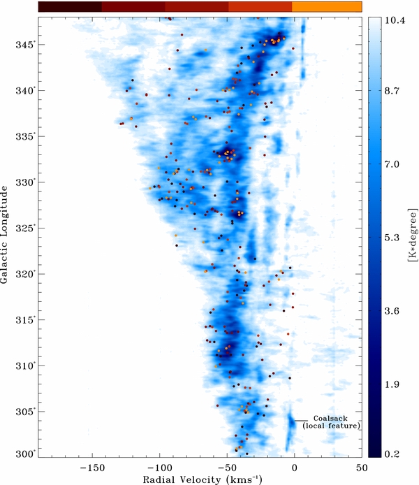
Figure 1. Longitude–velocity diagram of the Columbia University–Universidad de Chile CO Survey and IRAS point-like sources with FIR colors of UC H ii regions (Wood & Churchwell 1989; IRAS/CS sources) in the fourth Galactic quadrant. The longitude–velocity diagram of the CO emission was obtained by integrating the data set over b = ±2 0. The bluish color scale denotes values of antenna temperature as ∫TAdb. A brief summary of the survey parameters is presented in Table 1. For the IRAS/CS sources, the reddish color scale represents the FIR flux (94–704 Jy, brown; 728–1590 Jy, dark red; 1629–3561 Jy, red; 3598–8140 Jy, orange; and 8160–62,864 Jy, yellow). The kinematic information of the sources was obtained from the most complete currently available CS(2–1) survey of IRAS point-like sources with FIR colors characteristic of UC H ii regions (Bronfman et al. 1996), complemented by a new CS(2–1) unpublished survey (L. Bronfman et al. 2014, in preparation).
Download figure:
Standard image High-resolution imageTable 1. The CO Survey of the Southern Milky Way
| Galactic longitude | 300° to 348° | |
| Galactic latitude | −2° to +2° | |
| Velocity coverage | −166 km s−1 to +166 km s−1 | (300° ⩽l ⩽ 335°) |
| −180 km s−1 to +153 km s−1 | (335° ⩽l ⩽ 345°) | |
| −218 km s−1 to +144 km s−1 | (345° ⩽l ⩽ 348°) | |
| Sampling interval | 0125 |
(000 ⩽|b| ⩽ 075) |
| 0250 |
(075 ⩽|b| ⩽ 200) | |
| Telescope HPBW | 0147 |
|
| Velocity resolution | 1.3 km s−1 | |
| Sensitivitya | ΔTrms ⩽ 0.13 K | |
| Main beam efficiency | η = 0.82 |
Notes. A detailed description of the Columbia Southern Deep CO Survey of the Milky Way can be found in Bronfman et al. (1988b, 1989). aAt velocity resolution of 1.3 km s−1.
Download table as: ASCIITypeset image
In order to identify the largest molecular clouds in the longitude–velocity diagram, similar to the analysis done by Dame et al. (1986) for the first Galactic quadrant, a synthetic data set was generated using the ASM of the CO emission by Bronfman et al. (1988b) (see the inset in the lower left corner of Figure 2) and was subtracted from the observed CO data set, creating a LBV background-subtracted data cube. In this data cube, individual boxes were defined containing the main emission features. As a consistency check, we used the spatial and radial velocity distribution of the IRAS/CS sources to trace the extension of such structures in phase space. The physical information of GMCs was then derived from their spatial maps and spectra. A detailed explanation of the method utilized to define the clouds is presented in Appendix A. After the subtraction of the CO background emission, the largest molecular clouds appear as isolated structures, allowing us to assign a (v, b, l) box in phase space to each one of the 92 clouds presented in our catalog. GMCs in the IVQ are presented in Figure 2, a longitude–velocity diagram of the model-subtracted CO emission from the CO Survey in units of antenna temperature.

Figure 2. Giant molecular clouds in the fourth Galactic quadrant. The longitude–velocity diagram was obtained by integrating the model-subtracted CO data set across the Galactic plane over b = ±20. The blue color scale denotes values of ∫TAdb. The first contour is located at 0.25 K. The axisymmetric model of the background emission is presented in the inset in the lower left corner. The model was subtracted from the data in Figure 1 in order to isolate GMCs from their surrounding background. The result is shown here.
Download figure:
Standard image High-resolution imageThe observational information of each cloud, contained in its phase space, is utilized in deriving its physical parameters (radius, mass, etc.). Integrating the phase space box over its angular extension, the composite spectrum of the cloud TA(v) = ∑TA(v, l, b)ΔbΔl, with Δb = Δl = 0125, is generated, and a Gaussian profile is fitted to obtain the radial velocity center (Vlsr), the velocity width (Δv(FWHM)), and intensity (ICO = ∫T(v)dv). In some cases because of the large velocity dispersion of the clouds, larger than the cloud separation, there is a partial blend of the CO profiles along the line of sight between two clouds. In those cases and in order to properly estimate the CO intensity for each individual cloud, two Gaussians were fitted simultaneously. An example of a two-Gaussian profile fit to recover the kinematic information and CO emission of the cloud GMC G333.625−0.125 is shown in Figure 3.
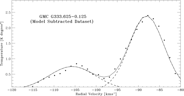
Figure 3. Composite spectrum for GMC G333.625−0.125. Filled circles represent the antenna temperatures in the composite spectrum, after subtraction of the axisymmetric model (ASM) of the CO background emission from the original data set. The solid line shows the results of the two-component Gaussian fit to the composite spectrum. The dashed lines show each individual Gaussian obtained in the fit procedure.
Download figure:
Standard image High-resolution imageThe physical parameters, such as position and angular size, are derived from the spatial map for each GMC. An example of the spatial map for a GMC in our catalog is presented in Figure 4, corresponding to GMC G331.500-0.125 (number 43 in Table 2). The limits in phase space were identified after the subtraction of the background model emission. The bluish color scale represents the CO intensity of the cloud (I(l, b) = ∑TA(v, l, b)Δv, with Δv = 1.3 km s−1), and the white square shows the CO peak intensity. Superimposed on the contours are 10 IRAS/CS sources associated with this cloud, identified as orange filled circles (the beam size for the CS sources is 50'' from the SEST Telescope at 100 GHz). The correlation of the point sources with the gas is evident, proving that massive star formation occurs primarily in GMCs. Similar spatial maps for all the clouds in our catalog are available on request.
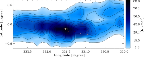
Figure 4. Spatial map for GMC G331.500−0.125. The bluish scale denotes values of CO intensity ∫TAdv. Orange dots denote the location of the IRAS/CS sources associated with this cloud in the present work. The white square shows the center of the cloud based on the CO peak intensity. All the intrinsic physical parameters for each cloud are derived from the information contained within the spatial map and composite spectrum of the cloud.
Download figure:
Standard image High-resolution imageTable 2. Giant Molecular Clouds in the Fourth Galactic Quadrant, within the Solar Circle
| Cloud | l | b | Vlsr | Δv | D | D.R. | R | Mvirial | M(H2) |
|---|---|---|---|---|---|---|---|---|---|
| (FWHM) | GMCs | ||||||||
| (°) | (°) | (km s−1) | (km s−1) | (kpc) | (pc) | log (M/M☉) | log (M/M☉) | ||
| 1 | 302.125 | +0.750 | −26.9* | 12.8 | 2.9 | Na,b | 74 | 6.41 | 6.13 |
| 2 | 305.250 | +0.375 | −35.1 | 11.4 | 3.7 | Na,b | 54 | 6.17 | 6.16 |
| 3 | 305.625 | −0.625 | −20.7 | 4.7 | 8.0 | Fc | 41 | 5.29 | 5.45 |
| 4 | 305.750 | +1.250 | −39.7* | 9.6 | 5.0 | Ta,d,e | 75 | 6.16 | 6.10 |
| 5 | 306.250 | −0.375 | −18.7 | 6.2 | 8.4 | Fb | 45 | 5.56 | 5.49 |
| 6 | 308.000 | −0.375 | −13.2 | 4.7 | 9.3 | Ff | 32 | 5.18 | 5.13 |
| 7 | 308.375 | +0.000 | −47.3* | 10.8 | 5.3 | Te | 69 | 6.23 | 5.89 |
| 8 | 309.000 | −0.250 | −10.8 | 12.8 | 7.3 | Fc,g | 65 | 6.35 | 5.93 |
| 9 | 309.125 | −0.375 | −40.2 | 11.5 | 3.7 | Na | 55 | 6.19 | 6.17 |
| 10 | 311.125 | +0.125 | −41.0* | 12.6 | 3.5 | Na,f | 66 | 6.34 | 6.41 |
| 11 | 311.875 | +0.125 | −47.1 | 9.4 | 4.1 | Nb,c,f | 58 | 6.04 | 6.19 |
| 12 | 312.375 | +0.125 | −11.5 | 10.9 | 10.5 | Fd | 62 | 6.19 | 6.00 |
| 13 | 312.500 | +0.125 | −49.4* | 6.5 | 5.7 | Te | 35 | 5.50 | 5.69 |
| 14 | 313.875 | −0.125 | −44.9 | 9.3 | 3.6 | Nc,g | 65 | 6.07 | 6.31 |
| 15 | 314.250 | +0.250 | −57.6 | 8.0 | 5.2 | Nf | 48 | 5.81 | 6.26 |
| 16 | 316.875 | +0.250 | −21.3 | 11.0 | 10.8 | Fc | 100 | 6.41 | 6.42 |
| 17 | 317.750 | +0.000 | −17.6 | 12.8 | 11.2 | Fc,f | 106 | 6.56 | 6.46 |
| 18 | 318.250 | −0.375 | −41.8 | 12.5 | 3.1 | Na,b,f | 73 | 6.38 | 6.45 |
| 19 | 319.375 | −0.125 | −20.3 | 7.5 | 11.3 | Ff | 100 | 6.07 | 6.18 |
| 20 | 319.750 | −0.375 | −8.4 | 14.9 | 12.3 | Fc | 82 | 6.58 | 6.27 |
| 21 | 320.375 | +0.125 | −7.8 | 9.0 | 12.5 | Fc,f | 82 | 6.14 | 6.11 |
| 22 | 320.750 | −0.375 | −66.3 | 11.7 | 4.8 | Nb | 32 | 5.97 | 6.00 |
| 23 | 320.750 | −0.250 | −55.3 | 5.6 | 3.9 | Na,b | 34 | 5.36 | 5.52 |
| 24 | 321.875 | +0.000 | −31.6 | 4.7 | 2.3 | Nc,f | 58 | 5.43 | 5.76 |
| 25 | 322.125 | +0.625 | −54.8 | 4.1 | 3.8 | Na,f | 23 | 4.92 | 5.32 |
| 26 | 323.500 | +0.000 | −65.5 | 4.0 | 4.5 | Nb | 33 | 5.04 | 5.50 |
| 27 | 323.500 | +0.625 | −45.3 | 10.7 | 3.2 | Nc,g | 22 | 5.72 | 5.23 |
| 28 | 323.750 | −0.250 | −52.3 | 8.0 | 3.6 | Nb,f | 43 | 5.77 | 5.78 |
| 29 | 326.625 | +0.625 | −42.1 | 9.6 | 3.0 | Na,b,f | 56 | 6.04 | 6.11 |
| 30 | 327.250 | −0.500 | −46.7 | 6.0 | 3.3 | Na,f | 16 | 5.08 | 4.99 |
| 31 | 327.250 | −0.250 | −62.3 | 10.2 | 4.2 | Nf | 52 | 6.06 | 6.08 |
| 32 | 327.750 | −0.375 | −70.7 | 11.3 | 4.6 | Nc,f,g | 65 | 6.24 | 6.22 |
| 33 | 328.250 | −0.500 | −45.0 | 11.9 | 3.2 | Na,b,f | 54 | 6.21 | 6.08 |
| 34 | 328.250 | +0.375 | −92.0 | 18.4 | 6.0 | Nf | 86 | 6.78 | 6.71 |
| 35 | 329.250 | +0.750 | −66.2 | 5.5 | ... | ... | ... | ... | ... |
| 36 | 329.375 | −0.250 | −74.3 | 7.7 | ... | ... | ... | ... | ... |
| 37 | 329.500 | +0.125 | −99.0 | 12.1 | 6.5 | Nf | 49 | 6.18 | 6.03 |
| 38 | 329.500 | +0.500 | −80.9 | 9.4 | 5.2 | Nf | 52 | 5.99 | 5.93 |
| 39 | 329.625 | +0.125 | −65.3 | 6.5 | ... | ... | ... | ... | ... |
| 40 | 330.000 | +1.000 | −86.2 | 4.7 | 5.5 | Nd | 21 | 4.98 | 5.02 |
| 41 | 331.125 | −0.500 | −65.0 | 10.6 | 4.3 | Na,b,f | 78 | 6.26 | 6.37 |
| 42 | 331.125 | +0.000 | −45.3 | 8.6 | 3.3 | Nf | 43 | 5.83 | 5.82 |
| 43 | 331.500 | −0.125 | −92.0 | 15.9 | 5.7 | Nb,f | 92 | 6.69 | 6.68 |
| 44 | 333.000 | +0.750 | −48.0 | 5.0 | 3.5 | Nf | 34 | 5.25 | 5.41 |
| 45 | 333.250 | −0.375 | −50.1 | 8.9 | 3.6 | Na,c,f | 67 | 6.05 | 6.29 |
| 46 | 333.625 | −0.125 | −88.1 | 9.6 | 5.4 | Nb,f | 75 | 6.17 | 6.30 |
| 47 | 333.875 | −0.375 | −105.0 | 12.2 | 6.3 | Nc,g | 70 | 6.34 | 6.19 |
| 48 | 334.125 | +0.500 | −62.2 | 12.2 | 11.1 | Fc,f | 95 | 6.47 | 6.57 |
| 49 | 334.250 | −0.125 | −40.4 | 8.2 | 3.1 | Nc,f | 64 | 5.96 | 6.12 |
| 50 | 336.000 | −0.875 | −48.3 | 7.4 | 3.6 | Nd | 23 | 5.44 | 5.25 |
| 51 | 336.875 | +0.125 | −74.2 | 16.0 | 10.8 | Fb,f | 121 | 6.81 | 6.84 |
| 52 | 337.000 | −1.125 | −42.2 | 7.4 | 3.3 | Nd | 29 | 5.53 | 5.49 |
| 53 | 337.250 | +0.000 | −116.1 | 14.2 | 6.7 | Nf | 75 | 6.50 | 6.37 |
| 54 | 337.750 | +0.000 | −55.1 | 18.2 | 11.7 | Fb,f | 104 | 6.86 | 6.94 |
| 55 | 338.000 | −0.125 | −94.1 | 16.2 | 5.7 | Nf | 57 | 6.50 | 6.03 |
| 56 | 338.250 | −1.000 | −111.5 | 7.4 | 6.4 | Nd | 37 | 5.63 | 5.36 |
| 57 | 338.625 | −0.125 | −119.1 | 8.4 | 6.7 | Nb,f | 69 | 6.01 | 6.07 |
| 58 | 338.875 | −0.625 | −45.7 | 6.8 | 3.6 | Nc | 30 | 5.47 | 5.44 |
| 59 | 339.000 | +0.625 | −60.5 | 10.6 | 4.4 | Na,f | 35 | 5.93 | 5.71 |
| 60 | 339.125 | +0.000 | −100.3 | 9.3 | 9.9 | Fc | 76 | 6.14 | 6.01 |
| 61 | 339.125 | +0.250 | −78.9 | 9.3 | 10.7 | Fc,f | 60 | 6.04 | 5.97 |
| 62 | 339.500 | +0.125 | −111.6 | 6.1 | 6.4 | Ng | 31 | 5.38 | 5.21 |
| 63 | 339.750 | −1.250 | −30.7 | 7.2 | 2.8 | Na,c,d | 33 | 5.56 | 5.51 |
| 64 | 340.250 | +0.000 | −122.1 | 8.6 | 6.8 | Ng | 77 | 6.07 | 6.14 |
| 65 | 340.375 | −0.375 | −42.9 | 12.3 | 3.6 | Na,c,f | 63 | 6.30 | 6.32 |
| 66 | 340.625 | −0.625 | −90.8 | 5.8 | 5.7 | Nc | 68 | 5.68 | 5.86 |
| 67 | 340.750 | −1.000 | −28.9 | 5.5 | 2.7 | Na,d | 25 | 5.20 | 5.31 |
| 68 | 341.000 | +0.000 | −101.1 | 6.5 | 6.0 | Nc,g | 49 | 5.64 | 5.43 |
| 69 | 341.375 | +0.250 | −24.3 | 8.6 | ... | ... | ... | ... | ... |
| 70 | 341.500 | −0.125 | −129.3 | 11.2 | 7.0 | Ng | 45 | 6.08 | 5.69 |
| 71 | 341.500 | +0.000 | −121.9 | 6.5 | 6.8 | Ng | 37 | 5.51 | 5.35 |
| 72 | 342.125 | +0.500 | −26.6 | 5.4 | 2.7 | Nc,f | 30 | 5.27 | 5.35 |
| 73 | 342.250 | +0.250 | −122.8 | 8.3 | 6.8 | Ng | 47 | 5.83 | 5.56 |
| 74 | 342.625 | +0.125 | −41.5 | 5.1 | 12.5 | Fb | 87 | 5.67 | 6.12 |
| 75 | 342.750 | −0.500 | −27.0 | 7.7 | ... | ... | ... | ... | ... |
| 76 | 342.750 | +0.000 | −79.8 | 13.2 | 5.4 | Nc,g | 75 | 6.44 | 6.35 |
| 77 | 343.250 | +0.125 | −120.1 | 10.3 | 6.7 | Ng | 66 | 6.17 | 5.95 |
| 78 | 344.125 | −0.625 | −26.0 | 10.0 | 2.8 | Nf | 38 | 5.90 | 5.85 |
| 79 | 344.500 | +0.125 | −68.2 | 12.0 | 5.1 | Nf | 67 | 6.31 | 6.10 |
| 80 | 344.500 | +0.125 | −44.1 | 9.6 | 12.4 | Ff | 131 | 6.41 | 6.77 |
| 81 | 345.000 | −0.250 | −85.9 | 4.3 | 5.8 | Nc | 36 | 5.16 | 5.18 |
| 82 | 345.125 | −0.250 | −93.8 | 4.7 | 10.4 | Fc | 52 | 5.38 | 5.50 |
| 83 | 345.125 | +0.125 | −119.6 | 14.2 | 6.7 | Ng | 59 | 6.40 | 5.83 |
| 84 | 345.250 | −1.000 | −108.0 | 7.4 | 6.4 | Ng | 37 | 5.62 | 5.15 |
| 85 | 345.250 | −0.750 | −22.1 | 7.0 | 2.6 | Na,b | 32 | 5.52 | 5.52 |
| 86 | 345.250 | +1.000 | −13.7 | 10.1 | 1.8 | Na,b | 34 | 5.87 | 5.72 |
| 87 | 345.875 | +0.000 | −36.0 | 7.7 | 3.7 | Nc,f | 27 | 5.53 | 5.42 |
| 88 | 346.000 | +0.000 | −79.8 | 13.9 | 10.8 | Fc,f | 90 | 6.56 | 6.35 |
| 89 | 346.125 | −0.125 | −104.9 | 8.3 | 6.4 | Ng | 26 | 5.57 | 5.14 |
| 90 | 346.500 | +1.000 | −57.6 | 7.4 | 4.9 | Nc,d | 49 | 5.75 | 5.71 |
| 91 | 347.000 | +0.250 | −118.4 | 7.4 | 6.8 | Ng | 49 | 5.76 | 5.38 |
| 92 | 347.250 | +0.000 | −68.8 | 9.3 | 11.1 | Fc,f | 61 | 6.04 | 5.94 |
Notes. The following letters represent the method in which the two-fold distance ambiguity was removed: aSpatial association with optical objects from the RCW catalog (Rodgers et al. 1960) or visual optical counterparts (Caswell & Haynes 1987). bIRAS/CS source associated to the cloud with distance ambiguity already removed. cObservational size-to-linewidth relationship (Larson's Law). dLatitude criterion. eCO radial velocity of the cloud close (|v| < 10 km s−1) to the tangential velocity. fPresence or absence of absorption features from species like H2CO or OH against the Hα continuum emission from H ii regions, or cold (10–30 K) H i absorption against the warm (100–104 K) H i continuum background. gContinuity of spiral arm. (*) The CO radial velocity of the cloud was corrected by +12.2 km s−1 in order to take into account the unusual velocity excess toward terminal velocities up to galactocentric longitude 312° reported by Alvarez et al. (1990). (...)The two-fold distance ambiguity could not be removed for these clouds.
2.2. Distance Determination
The determinations of heliocentric distances to GMCs are crucial to obtain many of their physical parameters. Currently, a huge effort is being made to obtain distances to massive-star-forming regions (such as water and methanol masers) in the northern hemisphere via trigonometric parallaxes (Brunthaler et al. 2011; The BeSSeL Survey), and it is planned to extend this work to southern hemisphere sources (Reid et al. 2009a). Since this is ongoing work, distances for southern massive-star-forming regions are not available yet. On the other hand, because of optical extinction in the Galactic disk, kinematic distances are usually the only ones available for objects beyond ∼3 kpc. Using the radial velocity of the source and a rotation curve (under the assumption of pure circular motion of the gas around the Galactic center), a kinematic distance to the source can be determined. In the outer Galaxy, given the radial velocity of the source, a unique kinematic distance can be assigned to it. This is not the case for the inner Galaxy, where, because of geometric effects, the radial velocity of the source can come from two different places along the same line of sight. This geometric effect is known as the twofold distance ambiguity of the inner Galaxy. After the determination of the two possible kinematic distances for a source within the solar circle, the distance ambiguity must be removed in order to calculate distance-dependent physical parameters. In this simple way, distances can be obtained for GMCs in our catalog.
In order to estimate the kinematic distances to the GMCs in the present work, we adopt the rotation curve derived by Alvarez et al. (1990) from the same data set analyzed here, assuming a heliocentric distance to the Galactic center of R☉ = 8.5 kpc and a circular velocity of the local standard of rest Θ☉ = 220 km s−1:

Effects such as blending along the line of sight and deviations from the common assumption of pure circular motion are among the main sources of uncertainty in kinematic distances. Large-scale streaming motions have been observed in a number of regions (Burton 1988; Brand & Blitz 1993). They produce deviations from pure circular motion and may introduce uncertainties of up to 5% in the estimation of galactocentric radii with corresponding uncertainties in the estimated heliocentric distances that may go from 0.6 to 1.7 kpc if the streaming motion is along the line of sight (Luna et al. 2006). There are also several good examples in the fourth Galactic quadrant of large-velocity perturbations caused by the action of energetic events such as the large hole in the longitude–velocity diagram at 325°, −40 km s−1, attributed by Nyman et al. (1987) to a single event causing multiple supernova explosions and stellar winds.
On the basis of measurements of trigonometric parallaxes and proper motions of high-mass star-forming regions in the Galactic plane, Reid et al. (2009b) investigated deviations from a flat rotation curve by fitting a rotation curve of the form Θ(R) = Θ☉ + (dΘ/dR)(R − R☉), with Θ☉ = 254 km s−1 and R☉ = 8.4 kpc. Two values for the derivative dΘ/dR are obtained: 1.9 and 2.3. We tested both models and found no significant differences with the kinematic distances derived from the rotation curve in Equation (1). For both values of dΘ/dR, kinematic distances for clouds closer than 7.5 kpc (68 GMCs) are systematically underestimated. For ∼80% of these clouds, differences are less than 15%, on the order of the estimated errors. For the remaining 20% of these clouds, the largest difference is less than 30%. For clouds with heliocentric distances larger than 7.5 kpc (19 GMCs), the distance estimations are essentially the same (less than 5% difference).
The well-known twofold distance ambiguity is an important source of uncertainty in kinematic distances within the solar circle. In the present work, the ambiguity between far and near distance has been removed by several methods: (1) spatial association with optical objects and the existence of visual counterparts and (2) absorption measurements against H ii regions or IRAS/CS sources associated with the cloud for which the distance ambiguity has been solved. Other criteria, such as the latitude criterion (distance off the Galactic plane), the size-to-linewidth relationship, also known as Larson's first law (Larson 1981), and continuity of spiral arms, are complementary to the former criteria. The proximity of the CO radial velocity to the terminal velocity (|v| < 10 km s−1) is used to assign the tangent distance to the cloud. From the 92 GMCs previously defined, we were able to solve the twofold distance for 87 of them, which are the ones used in the following sections to analyze the properties of GMCs in our catalog. A detailed analysis of the methods utilized in removing the twofold distance ambiguity is presented in Appendix B.
After the distance ambiguity was removed for most of the GMCs in our catalog, we compared our distance ambiguity resolution criteria with those used for the 6.7 GHz methanol (CH3OH) masers by Green & McClure-Griffiths (2011, and references therein) as a consistency check. In most cases there is a good agreement between the distance assigned to the methanol masers and the distance determined in the present work for their parent GMCs. A detailed discussion of this consistency check can be found in Appendix B.
2.3. Physical Properties
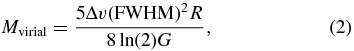
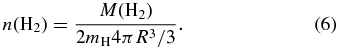
The physical parameters characterizing the GMCs identified here are summarized in Table 2. The first column represents the identification number of each GMC, from smaller to larger Galactic longitudes and from lower to higher Galactic latitudes. The second and third columns represent the Galactic longitude l and Galactic latitude b of the CO peak intensity in the spatial map of each GMC (as described in Figure 4). The fourth column represents Vlsr of each cloud, estimated from the Gaussian fit to its composite spectrum. Radial velocities with an asterisk were corrected by +12.2 km s−1 to take into account the anomaly in terminal radial velocities between l = 300° and 312° found by Alvarez et al. (1990). The fifth column is the linewidth Δv(FWHM) of each GMC composite spectrum. Column 6 gives the heliocentric kinematic distance D to each cloud. Column 7 gives the adopted distance (N = near, F = far, and T = tangent) and, as upper indexes, the criteria used in removing the distance ambiguity (see footnotes at the bottom of the table). Column 8 contains the radius for each GMC, defined as R = Rang × D, with Rang being the effective angular radius defined as  and Aang being the angular area. Since this criterion depends on the intensity threshold in the velocity-integrated spatial map, above which the observed position belongs to the cloud, Ungerechts et al. (2000) proposed to estimate the effective physical radius by weighting it by the CO intensity of the cloud. We keep our estimation of the effective physical radius mainly to be consistent with the previous northern catalog of Dame et al. (1986). Column 9 gives the virial mass Mvirial of GMCs in our catalog. Under the assumption of virial equilibrium, we estimate virial masses as follows:
where G is the gravitational constant. The last column contains the molecular mass M(H2) for each cloud estimated as follows:

A mean molecular weight per H2 molecule corrected for helium abundance of  (Allen 1973) is used. The χ factor is the Galactic average W(CO) to N(H2) conversion factor χ = 1.56 ± 0.05 × 10²⁰ (K km s−1)−1 cm−2 (Hunter et al. 1997) between the integrated CO main beam temperature WCO (WCO = ∫Tdv) and the molecular column density N(H2). The factor LCO represents the CO luminosity of the cloud estimated as
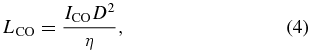
where η = 0.82 is the main beam efficiency correction of the antenna temperatures (Bronfman et al. 1989) and ICO (in units of K km s−1 sr2) is the integrated CO intensity of the cloud. To obtain ICO for each GMC, we perform the integral of T(v) over the Gaussian model fit for each cloud (ICO = ∫T(v)dv). However, the peak temperature of T(v) depends strongly on the level of the background emission model used to define the clouds (see Section 2.1). To remove such uncertainty, before computing ICO, the Gaussian fit is performed again over the original observed data set, but fixing Vlsr and Δv(FWHM) to the values obtained previously in the cloud definition process and leaving the peak temperature as the only free parameter. The value of ICO is then calculated from this new Gaussian fit and is independent of the level of the background model used to define the clouds. The procedure is further explained in Appendix A.
2.4. Statistical Properties
2.4.1. Size-to-linewidth Relationship
The theoretical interpretation of the apparently universal size-to-linewidth relationship of molecular clouds has been a matter of debate for many years, and often, different theoretical interpretations have been suggested. One of the first attempts was done by Larson (1981). They noticed that the power index (∼1/3) is similar to Kolmogorov's law of incompressible turbulence and argued that the observed nonthermal linewidths originate from a common hierarchy of interstellar turbulent motions and the structures in the clouds could not have formed by simple gravitational collapse. On the other hand, Solomon et al. (1987) argued that the Kolmogorov turbulent spectrum is ruled out by the "new" data with a power index of ∼1/2. They suggest that the size-to-linewidth relation arises from the virial equilibrium of the clouds since their mass, determined dynamically, agrees with other independent measurements and they are not in pressure equilibrium with a warm/hot interstellar medium. Recently, MHD models have shown that supersonic turbulence is sufficient to explain the observed slope of the size-to-linewidth relation and that self-gravity may be important on large and small scales (Evans 1999; Kritsuk 2007).
The size-to-linewidth relationship Δv(FWHM) = ARα for clouds in Table 2 is presented in Figure 5. A least-squares fit yields

The mean value of the FWHM for clouds in our sample is Δv(FWHM) = 9.3 km s−1, which implies a mean velocity dispersion of ∼4.0 km s−1. The mean physical radius of the clouds in Table 2 is R = 60 pc. The values A = 1.26 ± 0.35 and α = 0.50 ± 0.07 are in agreement with the values in Dame et al. (1986), A = 1.20 ± 0.22 and α = 0.50 ± 0.05 (since their estimations for the galactocentric radii do not scale linearly with R☉, we have explicitly adopted their radii estimates in Figures 5 and 6). Solomon et al. (1987) found a power-law relationship of the form σv = 1.0 ± 0.1S0.5 ± 0.05, where σv is the velocity dispersion of the cloud and S is its physical radius. The difference in the proportionality factor A is due to the different definitions of the physical radius of the clouds (geometrical average in their case) and the use of the velocity dispersion instead of Δv(FWHM) for the fit. The slope of the relationship is surprisingly similar to the value obtained in the present work, especially if the different methods employed in defining GMCs are considered. The same occurs in Scoville et al. (1987). They reported a relationship of the form σv = 0.5 ± 0.1S0.55 ± 0.05, which is close to our values within the error.
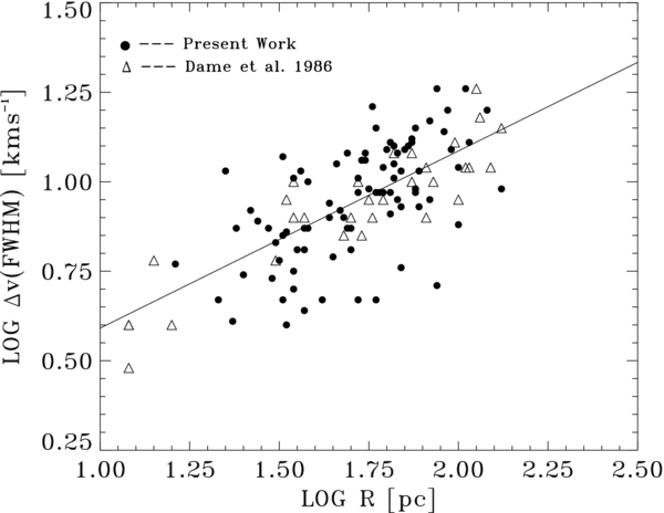
Figure 5. Logarithm of the observed linewidth Δv(FWHM) vs. the logarithm of the effective physical radius R of GMCs in Table 2 (filled circles) and for GMCs in the catalog of Dame et al. (1986) (open triangles). The straight line is a least-squares fit to the clouds in our catalog given by the equation log Δv(FWHM) = 0.10 + 0.50log R.
Download figure:
Standard image High-resolution image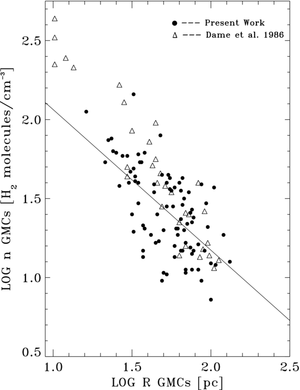
Figure 6. Logarithm of the H2 volume density corrected for helium n(H2) vs. the logarithm of the effective physical radius R for GMCs in Table 2 (filled circles) and for GMCs in the catalog of Dame et al. (1986) (open triangles). The straight line is a least-squares fit given by the equation log n(H2) = 2.95–0.89log R.
Download figure:
Standard image High-resolution image2.4.2. H2 Density-to-size Relationship
The H2 volume density n(H2) can be expressed as a function of the cloud's mass and radius:
The existence of a power-law relationship between n(H2) and R for molecular clouds (n(H2) = BR−β) was first reported by Larson (1981). This relationship is shown in Figure 6 for the clouds in our catalog. A least-squares fit to the physical quantities of GMCs in Table 2 gives

The dispersion of the data points is large. This is mainly due to the radius dependence in Equation (6) and the corresponding difficulties in defining such a radius. Nonetheless, a trend in Figure 6 is recognizable. The fit results are close to the values obtained by Grabelsky et al. (1987) for GMCs in the Carina spiral arm (B = 2.67 ± 1.75 × 10², β = 0.94 ± 0.16), in particular the slope (within error uncertainties). Since most clouds there do not suffer from the distance ambiguity and are very well defined, we believe that the determination of such an observational relationship should be more accurate for clouds in the outer Galaxy. On the other hand, the fit parameters are quite different from the values found by Dame et al. (1986) (B = 3.6 ± 1.2 × 10³, β = 1.3 ± 0.1), even if GMCs with densities greater than 100 cm−3 in their catalog are excluded and a new fit to their data is made, and there seems to be no easy way to reconcile both estimates. We believe this might be due to the different rotation curve utilized in their work.
2.4.3. Virial Mass to CO Luminosity Relationship and the W(CO) to N(H2) Conversion Factor
A relationship between virial mass and CO luminosity of the form Mvirial = CLCOδ is presented in Figure 7. A power-law fit represented by the dotted line yields

The correlation between virial masses and CO luminosities is evident from Figure 7. The fit parameters C = 13 ± 8 and δ = 0.90 ± 0.05 are similar to previous estimates in Solomon et al. (1987), C = 39 ± 12 and δ = 0.81 ± 0.03, although the slope in our relationship is closer to unity than in their work. The difference in the proportionality factor C is mainly due to the recovery of CO flux in our catalog. The well-behaved correlation makes the CO luminosity a good tracer of mass in the inner Galaxy.
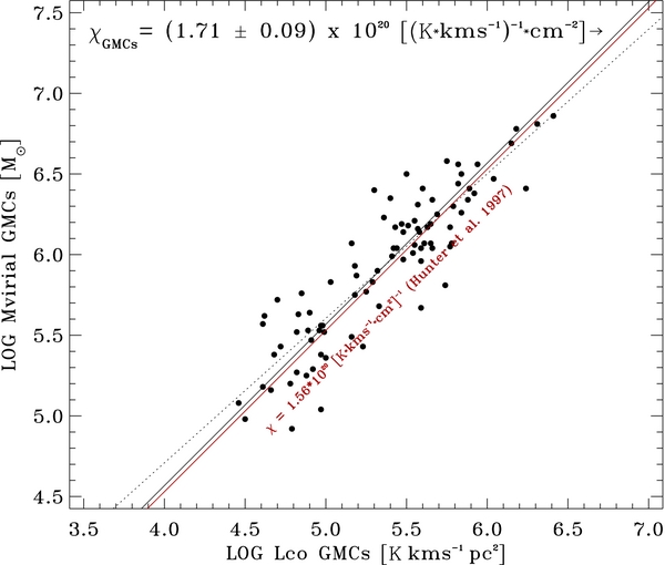
Figure 7. Logarithm of the virial mass vs. the logarithm of the CO luminosity for GMCs in Table 2. The dotted straight line is a least-squares fit given by the equation log Mvirial = 1.11 + 0.90 log LCO. The solid black straight line is a least-squares fit given by the equation log Mvirial = 0.57 + log LCO. The red straight line represents the W(CO) to N(H2) factor utilized in the present work (Hunter et al. 1997).
Download figure:
Standard image High-resolution imageA linear relationship between the virial mass and the CO luminosity might be used to estimate a W(CO) to N(H2) conversion factor for GMCs close to virial equilibrium. In such a case, the slopes found in Equations (5) and (7) are expected to follow the relationship α + β/2 = 1 (Dame et al. 1986; Bertoldi & McKee 1992). For our sample, this relationship yields α + β/2 = 0.95, supporting the idea that GMCs in our catalog are close to virial equilibrium. If we consider that the virial mass is close to the real mass of the clouds, the χ factor can be evaluated directly from the proportionality between the virial and molecular masses. The solid straight line in Figure 7 represents a least-squares fit procedure yielding Mvirial = (3.7 ± 0.2) LCO. The corresponding W(CO) to N(H2) average conversion factor, if GMCs are in virial equilibrium, is

This value is consistent within 10% with the χ conversion factor of 1.56 ± 0.05 × 10²⁰ (K km s−1)−1 cm−2 from Hunter et al. (1997) utilized here (see Figure 7).
From a theoretical point of view, Shetty et al. (2011) discussed possible variations in gas simulations of the χ factor for typical conditions in the Milky Way disk. They reported that the χ factor is not expected to be constant within individual molecular clouds, although in most cases it is similar to the Galactic value. From simulations, their best-fit model resembling typical conditions of the disk predicts an average value of χ = 2 × 10²⁰ (K km s−1)−1 cm−2, which is somewhat larger than our observational estimated value. Glover & Mac Low (2011, abstract) showed that "there is a sharp cut-off in CO abundance at mean visual extinctions Av ⩽ 3," where photodissociation becomes important. This is not the case for H2, which is argued to be controlled principally by the product of density and the metallicity and is insensitive to photodissociation. This could imply a different conversion factor for clouds and the intercloud medium. Ungerechts et al. (2000) studied GMCs in the Perseus spiral arm traced by the 12CO and 13CO lines. They adopt a factor χ = 1.9 × 10²⁰ (K km s−1)−1 cm−2, which is larger than the value of Hunter et al. (1997, p. 231), and they suggest that the "relatively large virial masses or equivalently, the low CO luminosities in relation to the linewidths show that χ could be even higher than the adopted value."
2.5. Molecular Mass Spectrum and Comparison with the Total Molecular Mass of the Galactic Disk
The molecular mass spectrum of clouds in Table 2 is shown in Figure 8. Following Williams & McKee (1997), we adopted a logarithmic mass bin interval of Δlog = 0.30 in constructing the mass spectrum of the clouds. Since the shape of the mass spectrum depends strongly on the selected mass bin (Williams & McKee 1997; Rosolowsky 2005), the adopted mass bin interval allows us to make a direct comparison between our results and the results presented in Williams & McKee (1997) in analyzing the catalogs of Solomon et al. (1987) and Scoville et al. (1987). The vertical dotted lines in Figure 8 indicate our completeness limit (around 1.3 × 10⁶ M☉), where about 75% of the molecular mass is concentrated toward the high-mass end of the spectrum, meaning that we are, in fact, detecting most of the molecular mass in the catalog. Error bars are estimated as  , where N is the number of clouds that fall into each mass bin. Triangles represent the central mass of each mass bin. A least-squares fit to the data is performed in the range indicated by the solid line. The dashed line is an extrapolation of the fit to the lower-mass end of the distribution. The least-squares fit yields
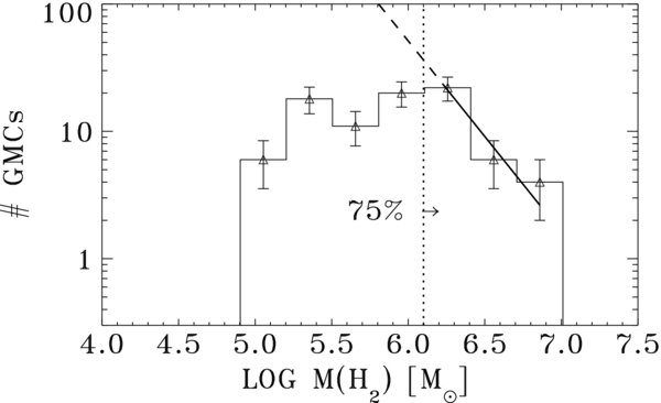
Figure 8. Mass spectrum for GMCs in Table 2. A least-squares fit has been made over the range indicated by the solid line, with the dashed line being an extrapolation to the lower-mass end of the spectra. The logarithmic mass bin is Δlog = 0.3. Small triangles represent the central mass in each mass bin, and the dotted line represents the 75% of the total molecular mass contained in the high-mass end of the distribution. The slope of the distribution is γ = 1.50 ± 0.40.
Download figure:
Standard image High-resolution imageThe mass distribution of GMCs determines how the molecular mass is distributed among GMCs. For the inner Galaxy, observational evidence has shown a slope of the mass spectrum for GMCs γ < 2 (Dame 1983; Casoli et al. 1984; Sanders et al. 1985; Solomon et al. 1987; Solomon & Rivolo 1989; May et al. 1997; Williams & McKee 1997; Blitz & Rosolowsky 2004; Rosolowsky 2005; Blitz et al. 2007). The value for the index of the mass distribution of GMCs in the inner Galaxy, γ = 1.50 ± 0.40 in the present work, γ = 1.81 ± 0.14 for the Solomon et al. (1987) GMC catalog, and γ = 1.67 ± 0.25 for the clouds in Scoville et al. (1987), strongly suggests that most of the molecular mass is concentrated toward the largest molecular clouds in the Galactic disk.
The total molecular mass in the form of GMCs in our catalog is M(H2) = 1.14 ± 0.05 × 10⁸ M☉. The most massive cloud in the catalog is GMC G337.750+0.000, with a molecular mass of M(H2) = 8.7 × 10⁶ M☉. This last result shows that that the molecular mass upper limit Mmax = 6 × 10⁶ M☉, established in other GMCs catalogs, may depend on the way GMCs are defined. From stability arguments it is clear that a mass upper limit must exist, but here we find it is higher than the previous value in the literature.
2.5.1. Comparison with Axisymmetric Model Mass
The total molecular mass obtained for all the clouds in our catalog is 1.14 ± 0.05 × 10⁸ M☉. The sum of the virial masses for all clouds is very similar, 1.21 ± 0.03 × 10⁸ M☉. Errors are estimated from the standard deviations of the physical parameters from the Gaussian fits. In comparison, the molecular mass derived from the axisymmetric analysis of Bronfman et al. (1988b) for the same region sampled here is 3.03 × 10⁸ M☉. Therefore, we account for only about 40% of the axisymmetric model mass in our cloud decomposition analysis. Such a difference was already detected for the first Galactic quadrant by Williams & McKee (1997), who estimated about 80% of the axisymmetric model mass not accounted for in the catalogs of Solomon et al. (1987) and Scoville et al. (1987).
A possible explanation for this result may arise from the χ conversion factor used here to determine the GMC mass, which is the same conversion factor, averaged over the whole Galactic plane, used to calculate the axisymmetric model mass. It is possible to postulate different conversion factors for the GMCs and the intercloud medium (ICM). For instance, using the same conversion factor, half of the total mass is in GMCs and the other half is in the ICM, but using a conversion factor for GMCs twice that for the ICM, one would obtain 2/3 of the mass in GMCs and 1/3 in the ICM. Such a difference between χGMCs and χICM is consistent with results obtained from comparing LTE column densities measured with 13CO with those obtained from CO observations of GMC and ICM regions (A. Luna et al. 2014, in preparation).
In terms of the distance, the molecular mass in our catalog is distributed as follows: 59% is contained in 64 clouds at the near distance and 39% in 20 clouds at the far distance (the remaining 2% is contained in the 3 clouds for which the tangent distance was assigned), reflecting the fact that the model of the CO background emission is less sensitive to the mass at the far distance. The beam dilution causes GMCs at the near distance to be more easily detected than the clouds at the far distance, but this difference is not too large, as shown by the percentage of molecular mass detected at the near and far distances.
3. GMCs AS TRACERS OF THE LARGE-SCALE STRUCTURE IN THE FOURTH GALACTIC QUADRANT: SPIRAL ARM FEATURES
In this section we examine the large-scale structure traced by the GMCs in our catalog. In longitude–velocity space, spiral arm features appear as opening loops as a consequence of the rotation of the Galaxy (Bronfman et al. 2000, Figure 5). Since we have already removed the distance ambiguity for the GMCs in our catalog, we attempt to reconstruct the spiral structure of the southern Galaxy, within the solar circle, by following the position of the clouds in both longitude–velocity space and in the Galactic plane.
3.1. Identification of Spiral Arm Features
The large-scale spiral structure can be inferred in the longitude–velocity diagram of the IVQ. Using the model-subtracted data set and location of giant molecular clouds in the longitude–velocity diagram (only clouds with their twofold distance ambiguity removed), we reconstruct a tentative picture of the spiral structure in the IVQ (Figure 9). Clouds with different colors are used for each spiral arm. We distinguish three main large-scale features across the Galactic plane: the Centaurus spiral arm (near and far sides traced by clouds in red and orange boxes, respectively), the Norma spiral arm (blue boxes for the near and far sides of the arm), and the 3 kpc expanding arm (black boxes for the near and far sides of the arm). We assign the cloud in the yellow box to the near side of the Carina spiral arm identified by Grabelsky et al. (1987). The clouds at positive velocities are tracing the far side of the Carina arm (Bronfman 1986; Grabelsky et al. 1988), and as they are beyond the solar circle, they are out of the scope of the present work.

Figure 9. Giant molecular clouds in the fourth Galactic quadrant as tracers of the large-scale spiral structure in the southern Galaxy. From the plot we identify three spiral arms: Centaurus (red clouds tracing the near side and orange clouds tracing the far side), Norma (blue clouds tracing the near and far sides of the arm), and the 3 kpc expanding arm (black box clouds tracing the near and far sides of the arm). On the basis of spatial coincidence, we also identify one cloud (yellow box) belonging to the well-known Carina spiral arm (Grabelsky et al. 1987). On the basis of the distribution of GMCs in the longitude–velocity diagram, a tentative picture of the limits in CO radial velocity and Galactic longitude of the spiral features is presented in the inset in the lower left corner. The limits are plotted over the CO data of the CO Survey.
Download figure:
Standard image High-resolution imageThe most prominent spiral feature in Figure 9 is by far the Centaurus spiral arm, very clearly traced by 50 GMCs in our catalog, over 40° in its near side (red boxes), and over 15° in its far side (orange boxes). The near side of the arm extends roughly from 305° to 348° and from −70 to −30 km s−1, while its far side extends roughly from 35° to 321° and from −20 to 0 km s−1. Close to the far-side velocity of the Centaurus arm is a well-known feature, the Coalsack at 303° and 0 km s−1.
The Norma spiral arm is shown as blue boxes in Figure 9, extending roughly from 327° to 348° and from −110 to −50 km s−1. The detection of the far side of the arm is particularly difficult in this case since at some spots far emission overlaps with near emission. Such is the case for GMC G334.125+0.500 (48 in Table 2). In the latitude–velocity maps of Bronfman et al. (1989), the near emission appears as wide lanes along the Galactic latitude, while the far emission has a small angular extension but is very extended along the velocity axis. The far side of the Norma arm also harbors the most massive clouds in our catalog, namely, GMC G336.875+0.125 and GMC G337.750+0.000. This statement would change if GMC G342.750+0.000 (76 in Table 2) had the wrong distance assignment. We adopted the near distance to this cloud using the evidence we have collected from the literature, but its distance ambiguity resolution is still not as solid as in other cases. If the cloud were indeed at the far distance, it would be associated with the far side of the 3 kpc expanding arm, and it would have the same molecular mass as the most massive cloud in our catalog, GMC G337.750+0.000, which is located at the far side of the Norma spiral arm. For further discussion on cloud 76, see Appendix B.
The 3 kpc expanding arm, the closest to the center of the Galaxy, is traced by clouds on its near side, between 335° and 348° and between −150 and −100 km s−1, and on its far side, between 345° and 348° and between −100 and −60 km s−1. The near side of the 3 kpc expanding arm has long been recognized in CO and 21 cm longitude–velocity diagrams as a nearly linearly feature in the range l = 348° to 12°, with an expanding motion of −53 km s−1 toward l = 0°. Recently, Dame & Thaddeus (2008) identified the far side of the arm over the same longitude range as a similar parallel feature displaced ∼100 km s−1 to positive velocities. At longitudes further from the Galactic center, the loci of the near and far arms are difficult to trace, and theoretical predictions vary widely (e.g., Cohen & Davies 1976; Romero-Gómez et al. 2011b). We find 13 clouds at l < 338°, with velocities and kinematic distances that suggest they trace the near side of the arm, and 4 more that may trace the far side (GMC 339.125+0.000, GMC 345.125+0.250, GMC 346.000+0.000, and GMC 347.250+0.000). Although the velocities of these clouds, −100 to −60 km s−1, are far below the velocity of the far arm at l > 348° as traced by Dame & Thaddeus (2008), just such a sharp drop in the far arm velocities at lower longitudes is predicted by the recent modeling of Romero-Gómez et al. (2011b). Furthermore, the derived distances of these clouds are consistent with that of the far arm as estimated by Dame & Thaddeus (2008).
In the following, we define limits in Galactic longitude and CO LSR velocity to produce spatial maps of each of the arms. In Figure 9, the inset in the lower left corner contains the radial velocity and Galactic longitude limits (orange lines) for each of the spiral arms overplotted on the CO data of the CO Survey. We set such limits following the distribution of the GMCs in the spiral arms. The limits in radial velocity and Galactic longitude of the boxes defined for the clouds belonging to the same spiral segment are used to establish the extension of the arm in longitude–velocity space. The view in Galactic longitude and latitude of the spiral arms is presented in Figure 10. In Figure 10, the CO Survey (without the subtraction of the axisymmetric model of the background emission) is used. The color scale of the gas represents the CO intensity (I(l, b) = ∑TA(v, l, b) × Δv) of the arms. The integration limits along the velocity axis were taken from the inset in Figure 9. The near and far sides of the 3 kpc expanding arm and the Norma arm are plotted on the same map. Overplotted on Figure 9 are the 284 IRAS/CS sources utilized in the present work (Section 4) to estimate the massive star formation rate per unit H2 mass and massive star formation efficiency. The sources are presented as filled circles in a reddish color scale representing the flux of each IRAS/CS source (see Figure 1). The correlation of the CO intensity and the distribution of IRAS/CS sources is evident, with the latter being very concentrated toward the plane within b = ±1° in all three arms. Since most parts of the arms are traced by GMCs, the role that they play as the places of most of the massive star formation in the Galactic disk is evident in Figure 9.

Figure 10. Spatial edge-on maps of the Galactic spiral arms obtained by integrating the CO data of the CO Survey across the corresponding velocity range presented in Figure 9 for each arm. Contours denote values of CO intensity I(l, b) = ∫TAdv. Each map has its own intensity color scale (except for the two maps showing the near side of the Centaurus arm, which share a common color scale), with the lowest intensity being at 7σ of the corresponding map, where σ is the characteristic intensity noise of the map. The spatial distribution of 284 IRAS/CS sources utilized in the present work along the spiral arms is also shown as superimposed filled circles.
Download figure:
Standard image High-resolution image3.2. Empirical Model of the Spiral Arms in the Southern Galaxy, within the Solar Circle
A face-on view of molecular clouds in the Galaxy, including our results and previous ones, is presented in Figure 11. In the fourth Galactic quadrant, GMCs in our catalog are plotted as filled circles with the color corresponding to its parent spiral arm (as defined in Figure 9) over the physical area covered in the present work (area filled with gray) between Galactic longitudes l = 300° and l = 348°. The size of the circles is proportional to the molecular mass of the GMCs (last column in Table 2). Also plotted are giant molecular clouds (black filled circles) from the catalog of Grabelsky et al. (1987), tracing the Carina spiral arm outside the solar circle. For the first Galactic quadrant, GMCs from the catalog of Dame et al. (1986) are plotted as black filled circles between Galactic longitudes l = 12° and l = 60°, tracing the Sagittarius, Scutum, and 4 kpc spiral arms, as identified by the authors. For the catalogs of Grabelsky et al. (1987) and Dame et al. (1986) their heliocentric distances were corrected by a factor of 0.85 to account for the different R☉ adopted, and for simplicity, molecular masses are those given by the authors. The dotted circle between the Sun and the Galactic center represents the "tangent distances" in the inner Galaxy, i.e., the distance at the CO terminal velocity. At the position of the Galactic center, the "molecular bar" is represented as a dash-dotted line. The parameters for the molecular bar were taken from Englmaier & Gerhard (1999) (for consistency with the work of Russeil 2003), with a radius of 3.5 kpc and an orientation angle of 225 measured from the Galactic center and in clockwise direction. Currently, there is a relatively broad consensus that our Galaxy is a moderate barred Galaxy and that the Galactic bar has two main components: a triaxial bulge (also referred as the "thick bar") inclined at an angle with values found in the literature between 15° and 30° and with a semimajor axis between 3.1 and 3.5 kpc long and a long "thin bar" inclined ∼45° (although more recent works suggest angles between 25° and 35°) with a semimajor axis of 4 kpc. The former is mainly traced by an old star population, while the latter is traced by a current star formation, such as methanol masers (Green et al. 2011; Romero-Gómez et al. 2011a, and references therein). Whether the angular separation between the thick and thin bars is real or just a projection artifact is still a matter of debate (Romero-Gómez et al. 2011a). In terms of star formation activity, an increase in star formation is expected where the thin bar and the 3 kpc expanding arm meet. Between Galactic longitudes of 345° and 351° and radial velocities of −30 and +10 km s−1, such an increase in star formation activity is observed in the methanol maser distribution of Green et al. (2011). It is interesting to notice that if one assumes a 45° inclination angle and a semimajor axis of 3.4 kpc for the thin long bar, the three GMCs at the far side of the 3 kpc expanding arm would match its southern end almost exactly.
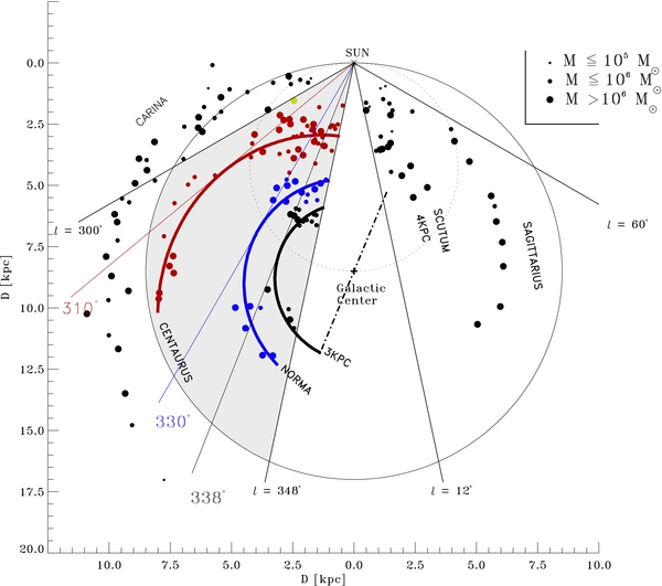
Figure 11. Spatial distribution (face-on view) of giant molecular clouds in the first and fourth Galactic quadrants. In the fourth Galactic quadrant, the 87 molecular complexes from Table 2 are drawn within the area covered in this work (gray filled area between l = 300° and l = 348°) and are associated by color with their corresponding spiral arm, as explained in Figure 9. The size of a circle is related to the molecular mass of the cloud. Toward lower Galactic longitudes, the molecular complexes tracing the Carina arm plotted as black filled circles are from Grabelsky et al. (1987). In the first Galactic quadrant, between l = 12° and l = 60°, the molecular complexes plotted as filled black circles are from Dame et al. (1986). The large dotted circle represents the tangent region within the solar circle, and the dash-dotted straight line represents the position of the Galactic bar taken from Englmaier & Gerhard (1999). The parameters for the three fitted spiral arms (seen as thick colored lines) in our catalog are summarized in Table 3. The fit was done by weighting each point by its galactocentric radius error.
Download figure:
Standard image High-resolution imageWe aim to quantify empirically the parameters describing the principal spiral features presented here. Following Russeil (2003), we fit a logarithmic spiral arm model to the positions of the clouds tracing each of the three spiral features seen in Figure 9 as

In the logarithmic spiral arm model, the origin of the reference frame to measure the angle ϕ (in radians) is set to the position of the Galactic center, and ϕ is measured clockwise, with ϕ = 0° at Galactic longitude l = 0°. The relationship in Equation (11) is defined by two parameters: the initial radius of the spiral arm r○ (kpc) and the pitch angle p, defined as the angle between the tangent to the corresponding galactocentric radius at a certain point in the spiral arm and the tangent direction to the arm at the same position. It is important to notice that the pitch angle is measured clockwise in the present work, yielding, by definition, only positive values, meaning that the −pϕ expression in Equation (11) is positive, and as a consequence, the galactocentric radius of the arm increases as the angle ϕ moves toward negative values, i.e., into the fourth Galactic quadrant. The model in Equation (11) is not intended to account for possible variations of the pitch angle along the spiral arm (Russeil 2003). In the fitting procedure, we weighted all clouds by the error in galactocentric radius. Other weights, such as molecular mass, yield the same results within error uncertainties. In Table 3 we summarize the results of the fit procedures for the spiral arms identified in our sample. The last column in Table 3 accounts for the tangent direction to each spiral arm seen from the Sun, i.e., as measured in Galactic longitude. The spiral arm models for the clouds in our catalog are plotted as thick colored lines in Figure 11. Tangent directions to the model spiral arms are plotted as colored straight lines.
Table 3. Fitted Parameters for the Logarithmic Spiral Arms Model in the Fourth Galactic Quadrant
| Spiral Arm | r○ | p | Tangent |
|---|---|---|---|
| (kpc) | (°) | (°) | |
| Centaurus | 5.40 ± 0.14 | 13.4 ± 2.0 | 310 |
| Norma | 3.72 ± 0.16 | 6.6 ± 2.3 | 330 |
| 3-kpc | 2.75 ± 0.16 | 5.6 ± 3.0 | 338 |
Download table as: ASCIITypeset image
In the following, we discuss the face-on view of GMCs in the Galaxy. The most prominent feature, as expected from Figure 9, is the Centaurus arm, traced over 10 kpc in the inner Galaxy. The tangent direction to the arm model in Table 3 around 310° is consistent with previous estimates (Alvarez et al. 1990; Bronfman 1992; Englmaier & Gerhard 1999). The arm is quite open and spatially closer to the Carina spiral arm than to the other spiral arm segments in the fourth quadrant. The pitch angle of this arm p = 134 is consistent with the values obtained by Russeil (2003) (∼11°) and Dame & Thaddeus (2011) (∼14°). The far side of the arm is better traced by GMCs than the near side, mainly because at far distances the CO background is much less prominent because of the beam dilution effects. The Norma spiral arm is the second major spiral feature in our catalog and contains the most massive clouds in our sample. The tangent direction to the model arm, ∼330°, is consistent with the values of 328° found by Alvarez et al. (1990) and Bronfman (1992). The pitch angle of the arm p = 66 in Table 3 is consistent with previous estimates (Russeil 2003, and references therein).
We pay special attention to the 3 kpc expanding arm. The far side of the 3 kpc expanding arm appears to be well traced by four clouds, but the spiral structure disappears at the near distances. We extended the fit of the logarithmic model for this arm to the position of the Galactic bar. The correlation between the clouds at the far distance and the position of the bar is evident and is also consistent with the distance determined by Dame & Thaddeus (2008) for the far side of the arm (11.8 kpc). The tangent direction for the arm, ∼338°, is also very consistent with the value of 337° found by Alvarez et al. (1990) and Bronfman (1992). A dense ridge of masers near l = 338° is identified as the tangent point of the 3 kpc expanding arm in the work of Green et al. (2011). Using the ATLASGAL 870 μm Survey, Beuther et al. (2012) identified an increase in the submillimeter clump distribution at l = 338° also attributed to the tangent point of the 3 kpc expanding arm. These results are fully consistent with the tangent direction we find from the logarithmic spiral model of the 3 kpc expanding arm. The GMCs associated with this spiral arm might be responding to the presence of a Galactic bar, causing their radial velocities to deviate from the assumption of pure circular motion. No previous estimation of the 3 kpc expanding arm pitch angle p ∼ 56 in Table 3 is found in the literature. On the observational side, the methanol maser distribution follows an oval structure in the longitude–velocity diagram that could be physically related to an elliptical structure in the face-on disk (Green et al. 2011). Such a structure accounts for the parallel lanes of the maser distribution at the far and near distances seen in the longitude–velocity diagram toward the Galactic center and, to some degree, also accounts for the tangent point at l = 338°. Beuther et al. (2012) show the 3 kpc expanding arm as a continuous elliptical structure in the Galactic disk following the work of Reid et al. (2009b). On the modeling side, Romero-Gómez et al. (2011a) applied for the first time the "invariant manifold" theory to model spiral arm features in the Galactic disk. Romero-Gómez et al. (2011b) approximately reproduce the observed longitude–velocity CO emission of the near and, to a lesser extent, the far sides of the 3 kpc expanding arm. Their PMM04-2 bar model naturally forms a continuous elliptical structure surrounding the composite Galactic bar (thick and thin bars). A continuous elliptical structure of the 3 kpc expanding arm seems to be also supported by the spatial distribution of GMCs associated with this arm in our catalog.
Concerning the region enclosed between the Norma and the 3 kpc expanding arms in Figure 11, Green et al. (2011) suggest that part of the Perseus arm could harbor some of the methanol masers found toward the tangent direction of the 3 kpc expanding arm and in the radial velocity range from −60 to −85 km s−1. They suggest that these sources could be attributed to the origin of the Perseus arm. In our catalog, only GMC G339.125+0.250, associated with the far side of the Norma arm, falls within this range. In Figure 11 we do not see any clear indication of the starting point of the arm in the region between the Norma and the 3 kpc expanding arms, the place where the starting point of the Perseus arm would be found according to the spiral arms models of Russeil (2003). Since our model is not sensitive to low-mass clouds at the far distance, if only low-mass GMCs were tracing the starting point of the Perseus arm, we would not be able detect them.
The transformation from longitude–velocity phase space to geometrical space in the inner Galaxy has to be done cautiously. Perturbations in the velocity field caused by density waves (Burton 1971) and energetic events, such as supernovae, as well as by the cloud-cloud velocity dispersion, introduce large uncertainties in the derived kinematic distances (typically between 10% and 20%). Such effects will inevitably wash out much of our description of the spiral structure in the derived distribution of clouds, even if the clouds are confined to a well-defined spiral pattern (Combes 1991). This is particularly true for the clouds tracing the 3 kpc expanding arm since its expanding velocity, around 53 km s−1, introduces large uncertainties into the position of the arm in phase and geometrical space. Another example of deviations of the pure circular motion is the hole at 329°, −60 km s−1 in the longitude–velocity diagram surrounded by molecular clouds with velocity differences of up to 30 km s−1 along the line of sight that, according to formaldehyde (H2CO) absorption measurements, are probably at the near side of the Centaurus arm. Usually, large variations in model parameters such as pitch angle, initial radius, and tangent direction are found depending on the tracer (21 cm emission, H ii regions, stellar population, etc.) used to identify the large-scale structure in the Galactic disk (Englmaier & Gerhard 1999; Russeil 2003).
Despite all difficulties involved in transforming CO radial velocities into heliocentric distances, the spiral structure in the southern Milky Way stands out clearly when traced by giant molecular clouds. In the present work, with a simple logarithmic spiral arm model, we reproduce some characteristics found by other authors, such as the tangent directions to the spiral arms in the southern Galaxy. More sophisticated models are necessary to account for the details of the parameters in each spiral arm. The purpose here is to test the consistency of the large-scale spiral structure traced by GMCs in the fourth Galactic quadrant with previous work.
4. MASSIVE STAR FORMATION RATE PER UNIT H2 MASS AND THE STAR FORMATION EFFICIENCY DERIVED FOR GMCs
There is close relationship between GMCs and massive stars in our study. While our CO Survey is the best available tracer of GMCs, the CS(2–1) survey is the best tracer of UC H ii regions. We find a close relationship between GMCs and massive stars in our study. Since most of the UV photons emitted by massive stars are absorbed and reemitted by the surrounding dust in the FIR part of the electromagnetic spectrum (Kennicutt 1998), the FIR emission of UC H ii regions is a good tracer of the massive star formation (Luna et al. 2006). On the other hand, the CS(2–1) emission requires high molecular gas densities, 104–105 cm−3, to become excited, resulting also in a good tracer of massive star formation regions. In order to estimate the massive star formation rate per unit H2 mass and the star formation efficiency of giant molecular clouds in our catalog, we use the catalog of IRAS point-like sources. The FIR flux of the UC H ii regions is obtained directly from the four bands (12, 25, 60, and 100 μm) of the IRAS point-like source catalog. Since the IRAS catalog does not provide the velocity information of the sources necessary to locate them along the radial velocity axis, we use the CS(2–1) line. We obtain the kinematic information of the UC H ii regions from the CS(2–1) survey by Bronfman et al. (1996) of IRAS point-like sources with FIR colors characteristic of UC H ii regions in the whole Galaxy complemented by a new survey to be published elsewhere. The new data amount to 19% of the detections.
There is a clear correlation between the molecular gas and the IRAS/CS sources, in particular, toward the position of spiral arms traced by GMCs. The IRAS/CS sources utilized in the present work are plotted over the CO emission in the longitude–velocity diagram from the CO Survey in Figure 1. The reddish color scale represents the FIR fluxes of the UC H ii regions. IRAS/CS sources with positive velocities were excluded from the present work since they are located outside the solar circle. From Figure 1 the correlation between the gas and the position of the IRAS/CS sources is evident, particularly their concentration at the position of the spiral features, such as the prominent Centaurus arm (the near side from 305° to 348° and from −70 to −30 km s−1 and the far side from 35° to 321° and from −20 to 0 km s−1). The 284 IRAS/CS sources are plotted in different velocity ranges, corresponding to spiral arms in the southern Galaxy, in Figure 10. We see that most of the sites of massive star formation are very concentrated within ±1° of the Galactic plane and correlate well to giant molecular clouds tracing the spiral arms. The 3 kpc expanding arm contains around 4% of the UC H ii regions in the present work. Concerning the Norma arm, two prominent regions of massive star formation appear at 3315 and between 336° and 338°. This spiral arm contains around 14% of the IRAS/CS sources. Since the near side of the Centaurus arm is the largest spiral segment in the longitude–velocity diagram, it contains most of the UC H ii regions in our sample (57% of the IRAS/CS sources). Important regions of massive star formation in this spiral arm appear between 310° and 313°, at 331°, and between 332° and 334°. The far side of the Centaurus arm contains around 4% of the IRAS/CS sources. Although these sources have small FIR fluxes, they are very luminous since they are located at the far distance of the spiral arm.
The first step in estimating the MSFR of the clouds in our catalog is related to the association of each IRAS/CS source with its parent GMC. The association between UC H ii regions and GMCs is established using the following criteria: (1) the Galactic coordinates (b, l) of the IRAS/CS source fall inside the spatial range defined for each GMC, and (2) the CS radial velocity of the IRAS/CS source falls within the 3× σv velocity range, where σv is the velocity dispersion of the parent GMC. We associated 214 sources (∼75% of the total 284 IRAS/CS sources within the covered area in this work) with their parent GMCs. The remaining 49 IRAS/CS sources either are associated with less bright GMCs not considered in our catalog or have peculiar velocities for their parental GMCs. Since these sources represent only ∼20% of the total number of IRAS/CS sources, we consider the remaining 75% to be a fair representation of the massive star formation within giant molecular clouds in our catalog. An example of IRAS/CS sources with their parent GMCs is found in Figure 4.
The FIR luminosity LFIR of embedded stars in giant molecular clouds is summarized in Table 4. The first column represents the GMCs identification (clouds). The second column shows the amount of UC H ii associated with the cloud. The third column contains the total FIR flux FIRAS of the massive-star-forming regions associated with each giant molecular cloud. The FIR flux of each UC H ii region was derived directly from the fluxes reported in the four bands of the IRAS point-like catalog (version 1) as follows:
The fourth column contains the FIR luminosity LFIR derived for each GMC as LFIR = FIRASD2, where FIRAS is the total FIR flux for each cloud and D is its distance. The fifth column contains the massive star formation efficiency of GMCs described in Section 4.2. In our sample, the total molecular mass of the GMCs that harbor at least one massive star formation region is ∼9.7 × 10⁷ M☉, which accounts for 85% of the total molecular mass in the form of GMCs, and of the 60 GMCs in Table 4 with at least one associated UC H ii region, 36 have molecular masses larger than 106 M☉. In general, the most massive clouds exhibit most of the massive star formation in the Galactic disk. The total FIR luminosity in Table 4 emitted by the UC H ii regions associated with giant molecular clouds is 3.66 × 10⁷ L☉. From Table 4, the Norma spiral arm concentrates most of the massive star formation in the southern Galaxy. The 11 giant molecular clouds in this arm account for a total FIR luminosity of 1.85 × 10⁷ L☉, equivalent to 50% of the total FIR luminosity contained in GMCs. GMC G337.750+0.000 (54 in Table 2), which belongs to the far side of this arm, is the most prominent massive-star-forming region in the inner fourth Galactic quadrant, with a FIR luminosity of 6.45 × 10⁶ L☉, around 35% of the total FIR luminosity in the Norma spiral arm.
Table 4. FIR Luminosity and Massive Star Formation Efficiency for GMCs
| Cloud | No. of Sources | FIRAS | LFIR | |
Cloud | No. of Sources | FIRAS | LFIR | |
|---|---|---|---|---|---|---|---|---|---|
| (L☉ kpc−2) | log (L/L☉) | (%) | (L☉ kpc−2) | log (L/L☉) | (%) | ||||
| 1 | 10 | 57344 | 5.69 | 2.4 | 37 | 4 | 32191 | 6.13 | 8.1 |
| 2 | 11 | 76319 | 6.02 | 4.8 | 38 | 4 | 13121 | ... | ... |
| 3 | 1 | 306 | 4.30 | 0.5 | 41 | 7 | 54382 | 6.00 | 2.8 |
| 4 | 1 | 1763 | 4.64 | 0.2 | 42 | 1 | 1462 | 4.19 | 0.2 |
| 5 | 1 | 1693 | 5.08 | 2.5 | 43 | 10 | 85494 | 6.45 | 3.8 |
| 8 | 3 | 1957 | 5.02 | 0.8 | 44 | 1 | 8433 | 5.00 | 2.5 |
| 9 | 3 | 6501 | 4.95 | 0.4 | 45 | 14 | 218249 | 6.45 | 9.2 |
| 10 | 8 | 30355 | 5.57 | 0.9 | 46 | 2 | 7361 | 5.34 | 0.7 |
| 11 | 3 | 17899 | 5.48 | 1.3 | 49 | 1 | 3017 | 4.46 | 0.1 |
| 13 | 1 | 1343 | 4.65 | 0.6 | 50 | 1 | 4492 | 4.76 | 2.1 |
| 14 | 3 | 4059 | 4.72 | 0.2 | 51 | 2 | 36413 | 6.63 | 4.0 |
| 15 | 3 | 9828 | 5.42 | 0.9 | 53 | 5 | 23309 | 6.02 | 2.9 |
| 16 | 1 | 1825 | 5.33 | 0.5 | 54 | 8 | 46858 | 6.81 | 4.8 |
| 17 | 1 | 797 | 5.00 | 0.2 | 57 | 1 | 4807 | 5.34 | 1.2 |
| 18 | 11 | 56481 | 5.73 | 1.3 | 59 | 1 | 3119 | 4.77 | 0.7 |
| 19 | 1 | 5874 | 5.88 | 3.2 | 61 | 1 | 2210 | 5.41 | 1.8 |
| 20 | 1 | 748 | 5.05 | 0.4 | 62 | 2 | 5697 | 5.37 | 9.4 |
| 21 | 2 | 13753 | 6.33 | 10.7 | 63 | 2 | 15141 | 5.07 | 2.4 |
| 22 | 2 | 16087 | 5.57 | 2.4 | 64 | 3 | 5286 | 5.39 | 1.1 |
| 23 | 1 | 6657 | 5.02 | 2.0 | 65 | 11 | 59526 | 5.88 | 2.4 |
| 24 | 1 | 321 | 3.24 | 0.0 | 67 | 2 | 26713 | 5.30 | 6.4 |
| 26 | 1 | 11122 | 5.35 | 4.7 | 69 | 1 | 1272 | ... | ... |
| 28 | 3 | 9132 | 5.08 | 1.3 | 74 | 2 | 5097 | 5.90 | 3.9 |
| 29 | 7 | 93905 | 5.93 | 4.2 | 76 | 1 | 2304 | 4.83 | 0.2 |
| 31 | 7 | 12227 | 5.33 | 1.1 | 78 | 5 | 22821 | 5.26 | 1.7 |
| 32 | 3 | 12550 | 5.43 | 1.1 | 79 | 1 | 13478 | 5.55 | 1.8 |
| 33 | 5 | 22562 | 5.36 | 1.3 | 80 | 1 | 254 | 4.59 | 0.0 |
| 34 | 7 | 55326 | 6.31 | 2.6 | 85 | 2 | 63312 | 5.64 | 8.5 |
| 35 | 1 | 1565 | ... | ... | 86 | 12 | 174892 | 5.77 | 7.2 |
| 36 | 2 | 6612 | ... | ... | 88 | 1 | 2196 | 5.41 | 0.7 |
Download table as: ASCIITypeset image
4.1. Massive Star Formation Rate per Unit H2 Mass
We calculate the massive star formation rate per unit H2 mass, defined as MSFR = LFIR/M, for GMCs in our catalog, following Bronfman et al. (2000). In Figure 12, the observational relationship between the FIR luminosity in Table 4 and molecular masses for GMCs in Table 2 is shown. For this plot, we used only FIR luminosities of GMCs from Table 4 that have more than one associated UC H ii regions to reduce the statistical error of the relationship. The colors of the filled circles are related to the spiral arms in Figure 9.

Figure 12. Logarithm of the far-infrared luminosity in Table 4 vs. the molecular mass of GMCs. Only clouds with more than one associated IRAS/CS source are included. The straight line is a least-squares fit given by log LFIR = −0.39 + log M(H2). Colors are associated with spiral arm features, as explained in Figure 9. Red crosses are GMCs 9 and 14 in Table 2, which belong to the Centaurus spiral arm and were not considered in the fit. The straight line in the upper right square is a least-squares fit given by log LFIR = −0.24 + log M(H2) to the four most massive GMCs in the figure. We notice that the most intense massive star formation activity takes place in the Norma spiral arm (blue filled circles).
Download figure:
Standard image High-resolution imageThe two red crosses in the plot are GMC G309.125−0.375 and GMC G313.875−0.125, which belong to the Centaurus spiral arm, and were left out of the fit in Figure 12 because of their deviation from the general trend. GMC G309.125−0.375 has neither other IRAS/CS sources in LBV space close to the clouds nor nondetections in the CS data, so the low FIR luminosity seems to be real and not an artifact of the criteria used to associate UC H ii regions with GMCs. For GMC G313.875−0.125, there are two IRAS/CS sources close to the cloud in (l, b, v) space, but they do not fulfill the association criteria. The total IRAS FIR flux of the sources is 3293 L☉ kpc−2, which would increase LFIR by a factor 1.8. Nonetheless, this increase would not reconcile the position of the cloud within the general trend in Figure 9. In addition, no nondetections in the CS data are present. A possible reason for the deviation of the clouds from the trend in Figure 9 could be related to some UC H ii regions "missing" during the process to select them using FIR colors in the IRAS catalog.
The massive star formation rate is obtained from a least-squares fit to the proportionality relationship between the FIR luminosity and molecular mass of GMCs, which yields LFIR = 0.41 ± 0.07 M(H2). Additionally, a least-squares fit to the four most massive (M(H2) > 3 × 10⁶ M☉) and most active (LFIR > 2 × 10⁶ L☉) star-forming GMCs of the sample, GMC G328.250+0.375, GMC G331.500−0.125, GMC G336.875+0.125, and GMC G337.750+0.000, which belong to the Norma spiral arm (blue filled circles in the region enclosed by the dotted lines), was performed, yielding LFIR = 0.58 ± 0.09 M(H2).
The clouds belonging to the far side of the Norma arm are, within our catalog, the most massive and have the highest massive star formation rate in the southern Galaxy. Bronfman et al. (2000) showed that the mean massive star formation rate per unit H2 mass is higher in the southern Galaxy than in the northern Galaxy, being around ∼0.21 L☉/M☉ for 0.2 ⩽ R/R☉ ⩽ 1 and around ∼0.28 L☉/M☉ for 0.4 ⩽ R/R☉ ⩽ 0.8 and having a peak around ∼0.41 L☉/M☉ for 0.5 ⩽ R/R☉ ⩽ 0.6 (without correction for helium abundance). They suggested that such an enhancement of massive star formation appears to be dominated by the presence of the Norma spiral arm, where a large fraction of the most FIR luminous sources are found.
In order to compare our results with those in Bronfman et al. (2000), we first divide their estimates by m(H2)*/m(H2) = 2.72m(H)/2m(H) = 1.36, where m(H2)* is the H2 molecular mass corrected for helium abundance utilized in this work. The clouds in Table 4 are located in the range 0.37 ⩽ R/R☉ ⩽ 0.94. Their MSFR is about a factor of 2 higher than one derived by Bronfman et al. (2000) for almost the same region of the Galactic disk (∼0.21 L☉/M☉ for 0.4 ⩽ R/R☉ ⩽ 0.8). The four most massive GMCs in the sample are located in the range 0.55 ⩽ R/R☉ ⩽ 0.60 in galactocentric radius and coincide with the position of the MSFR peak found by Bronfman et al. (2000). Their MSFR is also about a factor of 2 higher than the one found by Bronfman et al. (2000) at the peak of the distribution of embedded stars of ∼0.30 L☉/M☉ with galactocentric radii in the range 0.5 ⩽ R/R☉ ⩽ 0.6. This shows that most massive star formation activity in the southern Galaxy occurs not only in the Norma spiral arm but in its most massive clouds. It is interesting to notice that the factor of 2 difference between the MSFRs in GMCs found here and by Bronfman et al. (2000) for the average and peak values is the same difference we have between the molecular mass in the form of GMCs here and the axisymmetric model molecular mass estimated by Bronfman et al. (1988b). According to this evidence, it appears reasonable to use the massive star formation rate per unit H2 mass of the most massive clouds in the Norma spiral arm as a standard scale to compare the massive star formation activity in the rest of the Galaxy.
The massive star formation rates estimated here and in Bronfman et al. (2000) are a strict lower limit because only UC H ii regions contribute to it. Since the diffuse FIR emission from dust contained in the clouds is not considered in the IRAS point-like source catalog and some embedded OB star probably illuminate dust regions with large angular sizes, escaping from the identification as ultracompact sources, the total FIR flux derived for a particular cloud is a lower limit to the real value, giving a lower limit for the MSFR.
4.2. Massive Star Formation Efficiency
The values for the massive star formation efficiency of the GMCs in our catalog are given in the last column of Table 4. To derive the massive star formation efficiency we first transform the FIR luminosity of the clouds into the corresponding massive star formation rate  in units of M☉ yr−1. Following Luna et al. (2006), we convert the FIR-Infrared luminosity of the clouds as follows:
Using  computed in Equation (13), the massive star formation efficiency for GMCs in our catalog can be determined as
where τOB = 108 yr is assumed to be a typical lifetime for an OB star region (Luna et al. 2006, and references therein). The estimated massive star formation efficiencies shown in Table 4 are derived for the molecular mass of clouds in our catalog. All efficiencies derived here are a few percent of the available molecular mass of the clouds, and the average value is 3%. This is consistent with the values found in the literature (Mac Low & Klessen 2004; Luna et al. 2006; Zinnecker & Yorke 2007; McKee & Ostriker 2007). Our estimates reinforce the common idea that GMCs are inefficient in forming massive stars, implying that processes other than simple gravitational collapse must control the MSFR in the clouds.
5. SUMMARY
Using the Columbia University–Universidad de Chile CO Survey of the southern Milky Way, we present the first catalog of GMCs in the fourth Galactic quadrant, within the solar circle. Their average size, linewidth, and mass are estimated, and their statistical properties are determined.
5.1. GMC Identification and Physical Properties
We identify 92 molecular complexes in the inner southern Galaxy and remove the twofold distance ambiguity for 87 of them. The total molecular mass of GMCs is M(H2) = 1.14 ± 0.05 × 10⁸ M☉. The evidence in our catalog from the observational size to linewidth (Δv(FWHM)∝Rα) and size to H2 volume density (n(H2)∝R−β) relationships suggests that GMCs are close to virial equilibrium (α + β/2 = 0.95). The mass spectrum of the clouds (slope γ = 1.50 ± 0.40) shows that most of the molecular mass is concentrated in the high-mass end of the distribution. For the total molecular mass in our sample, 60% is located at the near distance, while the remaining 40% is at the far distance. The completeness limit of the molecular mass spectrum is at 75% of the total mass.
5.2. Total GMCs Mass and Axisymmetric Model
The total molecular mass of GMCs in our catalog accounts for 40% of the molecular mass derived from the axisymmetric analysis of the H2 volume density in the fourth Galactic quadrant, while in previous studies it was only 20%. From the virial analysis, we estimate an average W(CO) to N(H2) conversion factor GMCs χGMCs = 1.71 ± 0.09 × 10²⁰ (K km s−1)−1 cm−2, which is consistent with the Galactic average value χ = 1.56 ± 0.05 × 10²⁰ (K km s−1)−1 cm−2 (Hunter et al. 1997). The average Galactic value of the conversion factor in Hunter et al. (1997) is estimated for both cloud and intercloud media simultaneously. A higher conversion factor for GMCs and a lower conversion factor for the intercloud medium could also reproduce the estimated average Galactic value and increase the molecular mass of GMCs, reducing the difference even further.
5.3. Large-scale Spiral Structure
We trace here three large-scale spiral arms within the solar circle: the Centaurus, Norma, and 3 kpc expanding arms. The Carina arm is not traced because of its wide latitude. After fitting a logarithmic spiral arm model for each of the arms, tangent directions are found to be at roughly 310°, 330°, and 338°, respectively. These values are consistent with previous determinations of the tangent directions done by Alvarez et al. (1990) and Bronfman (1992). The Centaurus arm is the most prominent feature in the southern Galaxy. Its pitch angle p = 134 is large compared to the pitch angles of the Norma (p = 66) and 3 kpc (p = 56) arms. The spatial maps of the arms show that the molecular gas contained in GMCs and UC H ii regions (IRAS/CS sources) are tightly correlated, with the Norma spiral arm being the feature with the most massive clouds in our sample. The positions of the far clouds in the 3 kpc expanding arm converge to the location of the far side of the arm traced in Dame & Thaddeus (2008) down to l = 348°.
5.4. Massive Star Formation Rate for GMCs
Massive stars form in GMCs. Making use of the CS(2–1) survey (Bronfman et al. 1996) toward IRAS point-like sources with FIR colors characteristic of UC H ii regions (Wood & Churchwell 1989) and a new unpublished CS(2–1) survey, we analyzed massive star formation GMCs. The total molecular mass of GMCs with massive star formation activity accounts for 85% of the total molecular mass in our sample, and 60% of them have masses larger than 6 × 10⁶ M☉. From the spiral features identified in our catalog, the Norma spiral arm is the most active in forming massive stars. The GMCs in this arm have a total FIR luminosity of 1.85 × 10⁷ L☉, equivalent to 50% of the total FIR luminosity in our sample. GMC G337.750+0.000 is the most prominent massive-star-forming region in the inner southern Galaxy, with a FIR luminosity of 6.45 × 10⁶ L☉, equivalent to 35% of the total FIR luminosity in the arm. The observational evidence is consistent with the idea that, in general, the most massive clouds exhibit most of the massive star formation in the Galactic disk.
The massive star formation rate per unit H2 mass and the massive star formation efficiency are estimated for GMCs in our catalog. From the molecular mass of GMCs in our sample, the massive star formation rate is 0.41 ± 0.06 L☉/M☉. A separate estimation for the most massive and most active massive-star-forming GMCs in our sample, GMC G328.250+0.375, GMC G331.500−0.125, GMC G336.875+0.125, and GMC G337.750+0.000, which belong to the Norma spiral arm, yields MSFR = 0.58 ± 0.09 L☉/M☉.
The MSFR in GMCs is about a factor of 2 higher than the values derived for the Galactic plane of ∼0.21 L☉/M☉ in the range 0.4 ⩽ R/R☉ ⩽ 0.8 and peak value of ∼0.31 L☉/M☉ for 0.5 ⩽ R/R☉ ⩽ 0.6 (where part of the Norma arm is located) derived by Bronfman et al. (2000) after a correction for helium abundance is applied to their results. The discrepancy could be explained in terms of the molecular mass difference between GMCs in the present catalog and the molecular mass derived from the axisymmetric model analysis done by Bronfman et al. (1988b). We derive an average massive star formation efficiency for GMCs of ∼3% of their available molecular mass.
We gratefully acknowledge Professor Patrick Thaddeus for his seminal contributions to this work. We thank Hector Alvarez for his early help with the analysis. We remember Professor Jorge May (deceased) for his unconditional dedication to this project. P.G. and L.B. acknowledge support from Basal Center for Astrophysics and Associated Technologies PFB-06.
APPENDIX A: AXISYMMETRIC MODEL SUBTRACTION
A.1. Axisymmetric Model
In order to isolate the largest molecular clouds in the fourth Galactic quadrant from the CO background emission in which they are immersed, similar to the work of Dame et al. (1986), an axisymmetric model of CO background emission was generated and subtracted from the full three-dimensional LBV observed CO data set. We assumed that the background emission follows the same radial distribution of the molecular mass in the fourth Galactic quadrant determined by Bronfman et al. (1988b). Following Dame et al. (1986), the background level was adjusted so that 65% of the nonlocal (|v| < 20 km s−1) emission was removed from the survey.
On large scales, the effect of subtracting the axisymmetric model from the CO data set can be observed in Figure 13, which shows standard longitude–velocity diagrams at Galactic latitude b = 0° for CO and 13CO emission. Figures 13(a)–(c) show CO(1–0) emission from the Columbia CO Survey, CO(1–0) emission of the CO Survey with the axisymmetric model subtracted, and 13CO(1–0) emission from Bronfman et al. (1988a), respectively. The inset in the lower left corner in panel (a) represents the axisymmetric model subtracted from the CO data to produce the longitude–velocity diagram in panel (b). The emission of the rare 13CO isotope is less saturated than the CO line, which is a better molecular mass tracer at high densities (∼103 cm−3), and its narrow line facilitates separation of individual clouds along the velocity axis (Dickman 1978; Frerking et al. 1982; Liszt et al. 1984; Liszt 1995). From Figure 13 it is evident that the subtraction of the background model from the CO data set dramatically improves the similarity between the 13CO and 12CO longitude–velocity diagrams, suggesting that such a subtraction effectively distinguishes the clouds from the CO background in which they are immersed.
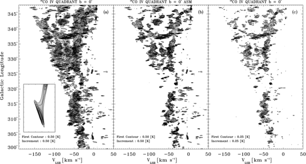
Figure 13. Longitude–velocity diagrams of CO and 13CO emission at b = 0° in the fourth Galactic quadrant. (a) CO observations from the CO Survey. The inset in the lower left corner shows the axisymmetric model subtracted from the CO data. The first contour in the model inset is at 0.5 K, and contour intervals are at 0.1 K. (b) Model-subtracted CO emission and (c) 13CO observations of the Galactic plane (Bronfman et al. 1988a). The subtraction of the axisymmetric model from the CO data dramatically improves the similitude between the 13CO (tracer of molecular densities higher than CO) and CO data.
Download figure:
Standard image High-resolution imageThe large-scale features are preserved after the model subtraction. The total CO intensity with no correction for the main beam efficiency (I = ∑TA(v, l, b)ΔvΔbΔl, with Δv =1.3 km s−1 and Δb = Δl = 0125) is 6.9 × 10³ and 2.4 × 10³ K km s−1 deg2 for the observed and subtracted model data sets, respectively, indicating that 65% of the total emission was removed. The subtraction of the model from the observed CO data set does not modify the overall shape of the intensity distribution, preserving the large-scale features of the emission. In Figure 14 the CO intensity distribution as a function of Galactic longitude (I(l) = ∑TA(v, l, b)ΔvΔb) is presented for the model-subtracted (CO MSD) and the observed (CO Survey) data sets. The tangent directions to spiral arms at 309°, 328°, and 337° (Bronfman 1992) are present in both data sets.

Figure 14. Intensity distribution along the Galactic longitude (I(l) = ∫TAdvdb) of the CO Survey (CO raw data) and the model-subtracted data set (MSD). Although a large fraction of the CO emission was removed from the observed data set by the model subtraction (63% of the nonlocal, |v| < 20 km s−1, emission), the intensity structure of the emission is preserved, and features like tangent directions toward spiral arms around 309° (Centaurus arm), 328° (Norma arm), and 337° (3 kpc expanding arm) (Bronfman 1992) appear in both data sets.
Download figure:
Standard image High-resolution imageA.2. Impact of the Model Subtraction on Individual Clouds
We investigate variations in the molecular mass M(H2) due to changes in the peak antenna temperature Tpeak from the recovery of the CO flux lost during the subtraction of the background axisymmetric model from the observed data set. In the following, we refer to the values calculated in the model-subtracted data set as "MSD" and the values determined for the clouds in our catalog as "GMCs." The values of Tpeak and M(H2) for both data sets are presented in Table 5. The relationship for each quantity between both data sets is shown in Figure 15. A least-squares fit between Tpeak(MSD) versus Tpeak(GMCs) and M(H2)(MSD) versus M(H2)(GMCs) yields


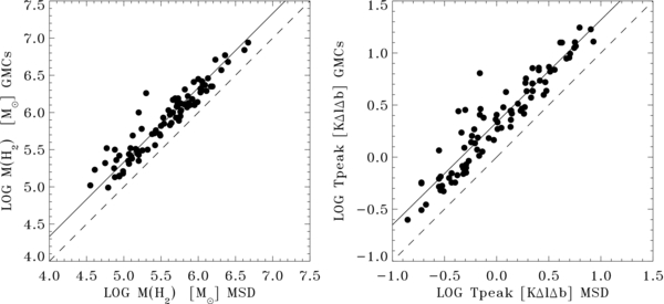
Figure 15. Left: molecular mass of GMCs vs. the molecular mass obtained from Gaussian fits in the MSD. The solid straight line represents a proportionality fit of the form log M(H2)GMCs = 0.33 + log M(H2)GMCs. Right: peak antenna temperature of GMCs vs. the peak antenna temperature obtained from Gaussian fits in the MSD. The solid straight line represents a power-law fit of the form log Tpeak(GMCs) = 0.33 + 0.98 log Tpeak(MSD). All values are summarized in Table 5.
Download figure:
Standard image High-resolution image
Table 5. Peak Antenna Temperature and Molecular Mass Derived from the Model Subtracted Data Set (MSD) and GMCs
| Cloud | l | b | MSD | GMCs | ||
|---|---|---|---|---|---|---|
| Tpeak | M(H2) | Tpeak | M(H2) | |||
| (°) | (°) | (KΔlΔb) | log (M/M☉) | (KΔlΔb) | log (M/M☉) | |
| 1 | 302.125 | +0.750 | 4.98 | 5.87 | 9.03 | 6.13 |
| 2 | 305.250 | +0.375 | 2.54 | 5.73 | 6.83 | 6.16 |
| 3 | 305.625 | −0.625 | 0.37 | 5.18 | 0.70 | 5.45 |
| 4 | 305.750 | +1.250 | 2.83 | 5.95 | 3.96 | 6.10 |
| 5 | 306.250 | −0.375 | 0.30 | 5.25 | 0.53 | 5.49 |
| 6 | 308.000 | −0.375 | 0.14 | 4.88 | 0.25 | 5.13 |
| 7 | 308.375 | +0.000 | 1.36 | 5.74 | 1.95 | 5.89 |
| 8 | 309.000 | −0.250 | 0.54 | 5.70 | 0.92 | 5.93 |
| 9 | 309.125 | −0.375 | 2.21 | 5.66 | 7.15 | 6.17 |
| 10 | 311.125 | +0.125 | 4.24 | 5.94 | 12.59 | 6.41 |
| 11 | 311.875 | +0.125 | 2.54 | 5.73 | 7.21 | 6.19 |
| 12 | 312.375 | +0.125 | 0.28 | 5.66 | 0.62 | 6.00 |
| 13 | 312.500 | +0.125 | 0.46 | 5.12 | 1.72 | 5.69 |
| 14 | 313.875 | −0.125 | 4.08 | 5.82 | 12.60 | 6.31 |
| 15 | 314.250 | +0.250 | 0.69 | 5.30 | 6.40 | 6.26 |
| 16 | 316.875 | +0.250 | 0.66 | 6.05 | 1.54 | 6.42 |
| 17 | 317.750 | +0.000 | 0.62 | 6.13 | 1.36 | 6.46 |
| 18 | 318.250 | −0.375 | 6.25 | 6.00 | 17.55 | 6.45 |
| 19 | 319.375 | −0.125 | 0.65 | 5.92 | 1.18 | 6.18 |
| 20 | 319.750 | −0.375 | 0.35 | 6.03 | 0.63 | 6.27 |
| 21 | 320.375 | +0.125 | 0.48 | 5.95 | 0.69 | 6.11 |
| 22 | 320.750 | −0.375 | 0.43 | 5.20 | 2.76 | 6.00 |
| 23 | 320.750 | −0.250 | 0.50 | 4.77 | 2.84 | 5.52 |
| 24 | 321.875 | +0.000 | 8.01 | 5.43 | 16.88 | 5.76 |
| 25 | 322.125 | +0.625 | 0.69 | 4.75 | 2.55 | 5.32 |
| 26 | 323.500 | +0.000 | 0.70 | 4.88 | 2.90 | 5.50 |
| 27 | 323.500 | +0.625 | 0.28 | 4.61 | 1.16 | 5.23 |
| 28 | 323.750 | −0.250 | 1.23 | 5.24 | 4.22 | 5.78 |
| 29 | 326.625 | +0.625 | 5.56 | 5.81 | 11.20 | 6.11 |
| 30 | 327.250 | −0.500 | 0.73 | 4.79 | 1.13 | 4.99 |
| 31 | 327.250 | −0.250 | 2.20 | 5.72 | 5.09 | 6.08 |
| 32 | 327.750 | −0.375 | 2.21 | 5.86 | 5.10 | 6.22 |
| 33 | 328.250 | −0.500 | 3.18 | 5.71 | 7.35 | 6.08 |
| 34 | 328.250 | +0.375 | 1.91 | 6.23 | 5.69 | 6.71 |
| 35 | 329.250 | +0.750 | 0.35 | ... | 0.96 | ... |
| 36 | 329.375 | −0.250 | 0.40 | ... | 0.98 | ... |
| 37 | 329.500 | +0.125 | 0.58 | 5.60 | 1.60 | 6.03 |
| 38 | 329.500 | +0.500 | 1.00 | 5.53 | 2.55 | 5.93 |
| 39 | 329.625 | +0.125 | 0.31 | ... | 1.01 | ... |
| 40 | 330.000 | +1.000 | 0.19 | 4.55 | 0.57 | 5.02 |
| 41 | 331.125 | −0.500 | 4.68 | 6.09 | 8.84 | 6.37 |
| 42 | 331.125 | +0.000 | 2.60 | 5.50 | 5.43 | 5.82 |
| 43 | 331.500 | −0.125 | 3.60 | 6.40 | 6.90 | 6.68 |
| 44 | 333.000 | +0.750 | 1.60 | 5.10 | 3.26 | 5.41 |
| 45 | 333.250 | −0.375 | 8.49 | 6.11 | 12.87 | 6.29 |
| 46 | 333.625 | −0.125 | 2.93 | 6.05 | 5.25 | 6.30 |
| 47 | 333.875 | −0.375 | 0.75 | 5.69 | 2.39 | 6.19 |
| 48 | 334.125 | +0.500 | 1.02 | 6.31 | 1.86 | 6.57 |
| 49 | 334.250 | −0.125 | 5.64 | 5.77 | 12.68 | 6.12 |
| 50 | 336.000 | −0.875 | 0.57 | 4.87 | 1.39 | 5.25 |
| 51 | 336.875 | +0.125 | 1.70 | 6.62 | 2.79 | 6.84 |
| 52 | 337.000 | −1.125 | 1.38 | 5.18 | 2.80 | 5.49 |
| 53 | 337.250 | +0.000 | 1.36 | 6.06 | 2.78 | 6.37 |
| 54 | 337.750 | +0.000 | 1.40 | 6.67 | 2.62 | 6.94 |
| 55 | 338.000 | −0.125 | 0.84 | 5.77 | 1.52 | 6.03 |
| 56 | 338.250 | −1.000 | 0.19 | 4.90 | 0.56 | 5.36 |
| 57 | 338.625 | −0.125 | 1.37 | 5.85 | 2.28 | 6.07 |
| 58 | 338.875 | −0.625 | 0.98 | 5.07 | 2.30 | 5.44 |
| 59 | 339.000 | +0.625 | 1.11 | 5.48 | 1.91 | 5.71 |
| 60 | 339.125 | +0.000 | 0.47 | 5.76 | 0.82 | 6.01 |
| 61 | 339.125 | +0.250 | 0.29 | 5.62 | 0.65 | 5.97 |
| 62 | 339.500 | +0.125 | 0.29 | 4.99 | 0.48 | 5.21 |
| 63 | 339.750 | −1.250 | 1.94 | 5.16 | 4.30 | 5.51 |
| 64 | 340.250 | +0.000 | 1.83 | 5.99 | 2.61 | 6.14 |
| 65 | 340.375 | −0.375 | 5.07 | 6.03 | 9.85 | 6.32 |
| 66 | 340.625 | −0.625 | 1.75 | 5.64 | 2.92 | 5.86 |
| 67 | 340.750 | −1.000 | 2.14 | 5.07 | 3.73 | 5.31 |
| 68 | 341.000 | +0.000 | 0.51 | 5.20 | 0.85 | 5.43 |
| 69 | 341.375 | +0.250 | 0.75 | ... | 1.73 | ... |
| 70 | 341.500 | −0.125 | 0.42 | 5.49 | 0.67 | 5.69 |
| 71 | 341.500 | +0.000 | 0.40 | 5.20 | 0.57 | 5.35 |
| 72 | 342.125 | +0.500 | 2.22 | 5.06 | 4.31 | 5.35 |
| 73 | 342.250 | +0.250 | 0.51 | 5.42 | 0.71 | 5.56 |
| 74 | 342.625 | +0.125 | 0.49 | 5.72 | 1.23 | 6.12 |
| 75 | 342.750 | −0.500 | 1.92 | ... | 3.61 | ... |
| 76 | 342.750 | +0.000 | 3.00 | 6.19 | 4.33 | 6.35 |
| 77 | 343.250 | +0.125 | 0.94 | 5.76 | 1.46 | 5.95 |
| 78 | 344.125 | −0.625 | 3.26 | 5.54 | 6.63 | 5.85 |
| 79 | 344.500 | +0.125 | 1.86 | 5.89 | 3.02 | 6.10 |
| 80 | 344.500 | +0.125 | 1.16 | 6.36 | 3.01 | 6.77 |
| 81 | 345.000 | −0.250 | 0.51 | 4.99 | 0.79 | 5.18 |
| 82 | 345.125 | −0.250 | 0.31 | 5.32 | 0.47 | 5.50 |
| 83 | 345.125 | +0.125 | 0.48 | 5.62 | 0.78 | 5.83 |
| 84 | 345.250 | −1.000 | 0.21 | 4.94 | 0.35 | 5.15 |
| 85 | 345.250 | −0.750 | 1.89 | 5.09 | 5.16 | 5.52 |
| 86 | 345.250 | +1.000 | 5.74 | 5.41 | 11.64 | 5.72 |
| 87 | 345.875 | +0.000 | 0.61 | 4.94 | 1.85 | 5.42 |
| 88 | 346.000 | +0.000 | 0.68 | 6.17 | 1.03 | 6.35 |
| 89 | 346.125 | −0.125 | 0.19 | 4.94 | 0.31 | 5.14 |
| 90 | 346.500 | +1.000 | 1.02 | 5.38 | 2.16 | 5.71 |
| 91 | 347.000 | +0.250 | 0.28 | 5.11 | 0.52 | 5.38 |
| 92 | 347.250 | +0.000 | 0.37 | 5.75 | 0.57 | 5.94 |
From Figure 15 we see that Tpeak changes linearly from the model-subtracted data set to the GMCs catalog. The differences between the subtracted model data set and the values of the GMCs in our catalog are only due to the CO flux recovery. After we have accounted for the loss of CO flux (see Section 2.3), the (average) Tpeak value increases by a factor of 2.14, as shown in Equation (A2), and this is directly mirrored in the increase of molecular mass shown in Equation (A3).
APPENDIX B: NOTES ON INDIVIDUAL GMCs
In this appendix we review the resolution for the twofold distance ambiguity for giant molecular clouds in our sample. After making an exhaustive search in the literature, we use nine criteria to distinguish between near and far distances. In most cases, more than one criterion is used to remove the distance ambiguity, and when all methods converge to the same solution, we assign the near or far distance to the cloud. The criteria are the following:
- a.Spatial association with optical objects of the RCW catalog (Rodgers et al. 1960) and visual counterparts for H ii regions (Caswell & Haynes 1987): usually, because of the high extinction in optical wavelengths, optical emission is detectable only for objects closer than 6 kpc within the Galactic plane, locating any cloud, with an optical counterpart, almost certainly at the near distance.
- b.IRAS/CS sources with distance ambiguity already removed associated with a GMC: in this case, the distance ambiguity resolution of the IRAS/CS source is assigned to the cloud, but the kinematic distance derived from the rotation curve is used to estimate all physical quantities of the parent GMC.
- c.Presence (or absence) of absorption features of species such as formaldehyde (H2CO) or the hydroxyl radical (OH) against the Hα continuum emission of H ii regions (Caswell & Haynes 1987) or H i absorption features in molecular clouds of the cold (10–30 K) atomic hydrogen against the warm (100–104 K) 21 cm continuum emission across the Galactic plane (Roman-Duval et al. 2009): In the first method, depending on the radial velocity of the recombination and absorption features and on the CO radial velocity Vlsr of the cloud, it is possible to distinguish between far and near distances to the cloud in several cases. For instance, if the absorption feature occurs at a radial velocity close to Vlsr (within 2σv) and it is smaller (less negative) than the radial velocity of the recombination line, the absorption can be interpreted as the cloud being in front of the H ii region absorbing the continuum emission, most likely at the near distance. On the other hand, if the LSR velocity of the absorption feature does not coincide with the LSR velocity of the cloud, the far distance is the most probable distance to the cloud. Because of the large linewidths of the H i recombination line (Δv(FWHM) ∼ 20–30 km s−1), the absorption features sometimes fall inside the recombination linewidth, making it hard to distinguish whether the emission originates in a location in the Galactic disk different from that of the recombination line. In those cases, the distance resolution solved by this technique should be taken with caution. The second method consists of comparing the H i self-absorption of the cold gas against the background of the H i warm continuum emission in the Galactic plane with the 13CO(1–0) emission at the same LSR velocity (Busfield et al. 2006; Roman-Duval et al. 2009). If H i self-absorption is identified to be at the same radial velocity of the 13CO(1–0) velocity for a particular source, the source lies almost certainly at the near distance since at the far distance the absorption feature would be "filled up" with the background of the H i continuum emission along the line of sight.
- d.Observational size-to-linewidth relationship (Larson's first law): the existence of an observational size-to-linewidth relationship for GMCs (Solomon et al. 1987; Scoville et al. 1987; Dame et al. 1986) can be used in some cases to distinguish between the near and far distances. Since the physical radius of a cloud is proportional to the distance, locating a cloud at the wrong position might yield an unrealistically large (more than 200 pc) or small (less than 10 pc) physical radius for the GMC. In regard to the velocity structure of the clouds, very massive GMCs at the far distance present an elongated structure along the radial velocity axis and a very reduced angular extension. An example of this can be found in the latitude-velocity maps in Bronfman et al. (1989) at 337250 between v = −90 km s−1 and v = −30 km s−1. If a cloud is located at a given distance (near or far), the physical radius of the cloud should be consistent with the overall trend in the observational size-to-linewidth relationship.
- e.Distance off the Galactic plane following the molecular gas distribution of Bronfman et al. (1988b): the position of a certain cloud relative to the Galactic plane in the azimuth direction can be used in some cases to distinguish between near and far distances. We examined the perpendicular projection of the distance to the clouds with respect to the plane and compared it with the distribution of the molecular gas in Bronfman et al. (1988b). The near distance is assigned to clouds that, being located at the far distance, strongly deviate (∼3σz) from the molecular gas distribution of the Galactic plane in the azimuth direction.
- f.Continuity of the near or far side of spiral arms: in a few cases, well-defined segments of spiral arms might also indicate the location of a particular cloud in the Galactic plane. Since spiral arms are seen as lanes of emission in the longitude–velocity diagram and the near and far sides of the arms are usually separated by a few tens of kilometers per second, clouds located at the far and near distances of the same arm are expected to be separated in LSR velocity well enough to be distinguishable from each other.
- g.CO radial velocity of a cloud lies close (|v| < 10 km s−1) to the tangential LSR velocity: since the difference between near and far distances decreases toward the tangent point to the line of sight, clouds that are close enough to the tangent LSR velocity at a given Galactic longitude l (Alvarez et al. 1990) are located at the tangent distance, i.e., at the distance where the galactocentric radius is minimum (Rgal = R☉sin l).
We explore the consistency of these criteria by comparing our distance determination results with those obtained for 6.7 GHz methanol (CH3OH) masers in the work of Green & McClure-Griffiths (2011) using the H i self-absorption method. We associated the methanol masers with their parent GMCs following the criteria explained for associating the IRAS/CS sources with GMCs. We only considered the methanol masers with the most solid distance ambiguity resolution (labeled with an "a" in column 5 of Table 2 in their work) that fall within the solar circle and within the range covered by the present work: l = 300°–348° and b = ±2°.
We found 20 GMCs with at least one associated methanol maser in our catalog. These GMCs in Table 2 are clouds 18, 28, 45, 49, 51, 63, 72, and 78, for which the maser information is fully consistent with the distance assigned to the corresponding GMC; clouds 9, 34, 35, 38, and 76, for which the methanol maser information contradicts our distance estimate but can be explained in terms of the sensitivity of our work to clouds less massive at the far distance; clouds 57, 64, and 73, which are associated with the near side of the 3 kpc expanding arm but for which the maser information puts them at the far distance; and clouds 14, 21, 33, and 54, for which there is an unexplained discrepancy between the methanol maser distance determination and our distance estimates. We include a detailed discussion of the methanol maser information for each GMC in the following notes on individual clouds.
1: IRAS/CS sources G300.969+1.152 and G301.116+0.966 associated with this cloud have as visual counterparts objects RCW65 (G301.0+1.2) and RCW66 (G301.1+0.9; Whiteoak & Gardner 1974; Shaver & Goss 1970; Caswell & Haynes 1987), locating this cloud at the near distance. The radial velocity of this cloud (Vlsr = −39.1 km s−1) was corrected by +12.2 km s−1 in order to take into account the anomalous terminal CO velocities between l = 300° and 312° in the fourth Galactic quadrant, as described in Alvarez et al. (1990).
2: IRAS/CS sources G305.085+0.062 and G305.194+0.036 are associated with optical object RWC74 (G305.1+0.15; Shaver & Goss 1970; Caswell & Haynes 1987; Caswell & Robinson 1974; Lockman 1979; Wilson et al. 1970), locating this cloud at the near distance. We did not correct the radial velocity of this cloud (Vlsr = −36.4 km s−1) by the anomalous +12.2 km s−1 radial velocity since it lies far (>15 km s−1) from the terminal velocity vterm = −55 km s−1 (Alvarez et al. 1990) at this Galactic longitude (l = 305250).
3: At the position of this cloud, no observations of absorption or recombination line emission were found in the literature. Locating this cloud at the near distance (1.9 kpc) yields a very small physical radius (∼10 pc). In this case, the absence of an optical counterpart at such a close distance is unlikely. Placing this cloud at the far distance yields a physical radius (∼42 pc) more consistent with the size-to-linewidth relationship. We adopt the far distance to the cloud.
4: The H ii region G305.678+1.607 has a visual optical counterpart (Caswell & Haynes 1987). The high latitude of this cloud (b = +1250) also suggests the near distance. The CO radial velocity (Vlsr = −51.9 km s−1) was corrected by +12.2 km s−1 in order to take into account the anomalous terminal CO velocities between l = 300° and 312°, as described in Alvarez et al. (1990). After this correction, we noticed that its galactocentric radius (Rgal = 6.88 kpc) is slightly smaller than the galactocentric radius at the tangent point of its line of sight (l = 305750) given by R☉sin (l) = 6.90 kpc. Since that is not allowed under the assumption of pure circular motion, the tangent galactocentric radius was chosen, and the corresponding heliocentric distance was assigned to this cloud.
5: On the basis of 13CO(1–0) and H i absorption observations, Busfield et al. (2006) assigned the far distance to the IRAS/CS source (G306.313−0.347) associated with this cloud. Since the H i data present no absorption at the 13CO(1–0) radial velocity of this source, the location of this cloud at the far distance is almost certain.
6: H ii region G308.092−0.432 presents deep H2CO absorption at −57 and at −13 km s−1 and recombination line emission at −17 km s−1. The absorption features and the absence of an optical counterpart place the source almost certainly at the far distance (Caswell & Haynes 1987), and by spatial and velocity coincidence, its parent GMC is also at the far distance.
7: The radial velocity of this cloud (Vlsr = −59.5 km s−1) was corrected by +12.2 km s−1 in order to take into account the anomalous terminal CO velocities between l = 300° and 312°, as described in Alvarez et al. (1990). After this correction, we noticed that its galactocentric radius (Rgal = 6.59 kpc) is slightly smaller than the galactocentric radius at the tangent point of its line of sight (l = 308375) given by R☉sin (l) = 6.66 kpc. Since that is not allowed under the assumption of pure circular motion, the tangent galactocentric radius was chosen, and the corresponding heliocentric distance was assigned to this cloud.
8: Given the large velocity dispersion of this cloud (Δv(FWHM) = 12.8 km s−1), putting this cloud at the far distance yields a physical radius (∼65 pc) more consistent with the observational size-to-linewidth relationship (Larson's first law) than the physical radius estimated from the near distance (∼30 pc). The continuity of the far side of the Centaurus spiral arm also suggests the far distance. Therefore, the far distance is assigned to this cloud.
9: H ii region G309.057+0.186 has a visual counterpart and exhibits recombination line emission at −47 km s−1 and no absorption, putting this cloud almost certainly at the near distance (Caswell & Haynes 1987). The 6.7 GHz methanol maser 308.754+0.549 is apparently associated with this cloud. The removal of its distance ambiguity by Green & McClure-Griffiths (2011) seems to contradict our distance determination for the GMC. Nonetheless, there is an explanation for the discrepancy. The maser is very close to a local maximum, far from the bulk of the integrated CO emission in the GMC's spatial map. The local maximum can be attributed to a less massive cloud at the far distance (if the distance determination of the associated maser is right) whose CO emission overlaps in phase space with the CO emission of the GMC at the near distance. Since our model is sensitive to only the most massive GMCs at the far distance, this is to be expected in some cases. In this sense, there is no contradiction to our determination of the GMC distance because the maser is associated with a different and less massive cloud at the far distance that we cannot properly isolate with the ASM subtraction technique applied in this work.
10: H ii region G310.994+0.389 is associated with catalog object RCW82 (G311.00+0.40; Caswell & Haynes 1987), locating this cloud at the near distance. The IRAS/CS source (G311.625+0.291; radial velocity from the CS(2–1) line is −56.2 km s−1) associated with this cloud presents H2CO absorption at −54 and −49 km s−1 and recombination line emission at −61 km s−1, also placing this cloud almost certainly at the near distance. The radial velocity of this cloud (Vlsr = −53.2 km s−1) was corrected by +12.2 km s−1 in order to take into account the anomalous terminal CO velocities between l = 300° and 312°, as described in Alvarez et al. (1990).
11: IRAS/CS source G311.899+0.084, associated with this cloud, presents a H i self-absorption feature at the same radial velocity as the recombination line emission, locating this cloud almost certainly at the near distance (Goss et al. 1970; Caswell & Robinson 1974; Caswell et al. 1975). IRAS/CS source G312.109+0.309 (radial velocity from the CS(2–1) line is −48.4 km s−1), also associated with this cloud, presents H2CO absorption and recombination line emission at −49 km s−1 (Caswell & Haynes 1987; Goss et al. 1970; Caswell & Robinson 1974; Caswell et al. 1975). Since no other absorption feature is present along the line of sight, this suggests the near distance. Given the velocity dispersion of the cloud (Δv(FWHM) = 9.4 km s−1), putting this cloud at the near distance yields a physical radius (59 pc) more consistent with the observational size-to-linewidth relationship (Larson's first law) than the physical radius estimated from the far distance (103 pc). Therefore, the near distance is assigned to this cloud.
12: Given the velocity dispersion of this cloud (Δv(FWHM) = 10.9 km s−1), putting this cloud at the far distance yields a physical radius (∼62 pc) much more consistent with the observational size-to-linewidth relationship (Larson's first law) than the physical radius estimated from the near distance (∼6 pc). Locating this cloud at the near distance yields a heliocentric distance of 0.9 kpc to the cloud. In this case, the absence of an optical counterpart at such a close distance is unlikely, also suggesting the far distance. The continuity of the far side of the Centaurus spiral arm also suggests the far distance. Therefore, the far distance is assigned to this cloud.
13: To assign a heliocentric distance to this cloud, we notice that its CO radial velocity (Vlsr = −61.6 km s−1) is very close to the CO terminal velocity (Vlsr = −65 km s−1) at the line of sight l = 312500 (Alvarez et al. 1990). Its galactocentric radius (Rgal = 6.07 kpc) is slightly smaller than the galactocentric radius at the tangent point given by R☉sin (l) = 6.27 kpc. Since that is not allowed under the assumption of pure circular motion, we extend the Galactic longitude range as suggested by Alvarez et al. (1990) and apply the +12.2  correction to the radial velocity of the cloud. The new galactocentric radius Rgal = 6.43 kpc is slightly larger than the one at the tangent point of the line of sight. Since the calculated galactocentric radii are very close before and after the correction (less than 5% difference), the galactocentric radius tangent to the line of sight was chosen, and the corresponding heliocentric distance was assigned to this cloud.
14: Given the velocity dispersion of this cloud (Δv(FWHM) = 9.3 km s−1), putting this cloud at the far distance implies a large physical radius (148 pc), causing the cloud to deviate from the observational size-to-linewidth relationship (Larson's first law). The continuity of the near side of the Centaurus arm also suggests the near distance for this cloud. We also notice that clouds at distances farther than 4 kpc usually subtend angular scales smaller than 1° (Green et al. 2011), while the angular size of the cloud in Galactic longitude is larger than 2° and in Galactic latitude it is larger than 1°. The 6.7 GHz methanol maser 314.320+0.112 is associated with this cloud. The removal of its distance ambiguity by Green & McClure-Griffiths (2011) contradicts our distance determination for its parent GMC. Inspecting the spatial distribution of the CO emission as well as the longitude–velocity diagram does not show any particular structure at the position of the maser that could be associated with a less massive cloud at the far distance. In this case, there is no obvious explanation to account for the contradictory evidence. We stick to our result and adopt the near distance to the GMC.
15: H ii regions G314.183+0.314 and G314.228+0.473 present H2CO absorptions features at −61 km s−1 and recombination line emission at −62 and −63 km s−1. We notice that the terminal velocity at l = 314250 is around −67 km s−1 (Alvarez et al. 1990), implying that the H ii regions are either at the near or the tangent distance. Since the absorption features at −61 km s−1 are close to the CO velocity of the cloud (Vlsr = −57.6 km s−1) and fall within its extension in radial velocity (Δv(FWHM) ∼ 8 km s−1), we interpret this as the cloud being in front of the H ii regions producing the absorption features, locating the cloud at the near distance.
16: At the position of this cloud, no observations of absorption or recombination line emission were found in the literature. We assign the far distance to the cloud on the basis of the observational size-to-linewidth relationship (Larson's first law). Putting the cloud at the near distance yields a very small physical radius (∼15 pc), causing the cloud to deviate far away from the general trend (Δv(FWHM) = 11.0 km s−1). We also notice that, in general, clouds at the far distance tend to have a small solid angle and small Galactic latitude (because of the distance projection) but still have, if the cloud is massive, a large velocity dispersion (Δv(FWHM) > 10 km s−1). This is, in fact, the case for this cloud.
17: On the basis of 13CO(1–0) and H i absorption observations Busfield et al. (2006) assigned the far distance to MYSO G318.2650−00.1269, which coincides in phase space with this cloud. Since the H i data present no absorption at the 13CO(1–0) radial velocity of the MYSO, the location of this source and its parent cloud at the far distance is almost certain. Also on the basis of H i absorption data, Urquhart et al. (2012) place H ii region G318.7251−0.2241 at the far distance. The observational size-to-linewidth relationship (Larson's first law) also suggests the far distance. Putting the cloud at the near distance yields a very small physical radius (∼13 pc), causing the cloud to deviate far from the general trend (Δv(FWHM) = 12.8 km s−1).
18: H ii region G320.153+0.780 is associated with optical object RCW87 (G320.20+0.80; Caswell & Haynes 1987; Wilson et al. 1970). H ii regions G319.874+0.770 and G316.808−0.037 present visual optical counterparts (Caswell & Haynes 1987; Churchwell et al. 1974). On the basis of 13CO(1–0) and H i absorption observations, Busfield et al. (2006) solved the distance ambiguity for IRAS/CS source G316.810−0.070, which is associated with this cloud, putting it at the near distance. On the basis of H i absorption data, Urquhart et al. (2012) place H ii regions G317.4122+0.1050 and G318.7748−0.1513 at the near distance. The 6.7 GHz methanol maser 318.050+0.087 is associated with this cloud. The removal of its distance ambiguity by Green & McClure-Griffiths (2011) confirms our distance determination for its parent GMC.
19: H ii regions G319.157−0.423 and G319.380−0.025, listed by Caswell & Haynes (1987), present H2CO absorption features at −20 km s−1 and recombination line emission at −22 and −14 km s−1, respectively. No optical counterparts were found. The authors put these sources at the far distance. Since the H2CO absorption radial velocity coincides with the CO radial velocity of this cloud (Vlsr = −20.3 km s−1), we locate this cloud at the far distance. On the basis of H i absorption data, Urquhart et al. (2012) place H ii regions G318.9148−0.1647, G319.1632−0.4208, and G319.3622+0.0126 at the far distance.
20: We assign the far distance to this cloud on the basis of the following: given the velocity dispersion of this cloud (Δv(FWHM) = 14.9 km s−1), putting this cloud at the near distance implies an unrealistically small physical radius (5 pc), causing the cloud to deviate from the observational size-to-linewidth relationship (Larson's first law).
21: H ii region G320.317−0.208 (possibly the same object as IRAS/CS G320.316−0.180) presents H2CO absorption at −11.4 km s−1 and recombination line emission at −11 km s−1 (Caswell & Haynes 1987). The same occurs with H ii region G320.379+0.139, which presents H2CO absorption and recombination line emission at the same velocity, −3 km s−1 (Caswell & Haynes 1987). These observations and the lack of an optical counterpart place this cloud almost certainly at the far distance. Putting this cloud at the near distance leads to an unrealistic physical radius of ∼4 pc. The 6.7 GHz methanol maser 320.123−0.504 is associated with this cloud. The removal of its distance ambiguity by Green & McClure-Griffiths (2011) contradicts our distance determination for its parent GMC. We notice that the maser coincides spatially and spectrally with IRAS/CS G320.124−0.501, associated with this cloud. In the longitude–velocity diagram, there is no other CO emission feature around this GMC to which the maser could be associated, so the evidence suggests that the maser is indeed at the far distance. Given the strong evidence we have to put this cloud at the far distance, we believe that the distance determination of the maser may be wrong, so we stick with our distance estimate with the GMC at the far distance.
22: The IRAS/CS source (G320.252−0.296) associated with this cloud presents H2CO absorption at −13 km s−1 and recombination line emission at −68 km s−1 (Caswell & Haynes 1987). The absence of absorption features between the IRAS/CS radial velocity and the terminal velocity at its line of sight (vterm ∼ −76 km s−1) suggests the near distance for the source. For IRAS/CS source G320.332−0.307, Georgelin & Georgelin (1976) place it at the near distance, applying the criterion of the continuity of the arms. We adopt the near distance to the cloud.
23: H ii regions G321.038−0.519 and G321.105−0.549 have visual optical counterparts (Caswell & Haynes 1987; Wilson et al. 1970). IRAS/CS source G321.057−0.520 is associated with optical object RCW91 (G321.20−0.50; Whiteoak & Gardner 1974; Caswell & Haynes 1987), locating this cloud at the near distance.
24: H ii region G324.192+0.109 presents several H2CO absorptions behind −92 km s−1 (Caswell & Haynes 1987), with no features between the recombination line velocity and the terminal velocity, locating this region at the near distance. One of the H2CO absorption features of this region occurs at −29 km s−1, very close to the CO radial velocity of this cloud (Vlsr = −31.6 km s−1), locating this cloud in front of the H ii region at the near distance. We also notice that, given the velocity dispersion of the cloud (Δv(FWHM) = 4.7 km s−1), putting this cloud at the far distance implies an unrealistically large physical radius (280 pc), causing the cloud to deviate from the general trend of the observational size-to-linewidth relationship (Larson's first law). The large angular extension of this cloud also supports the near distance.
25: H ii region G322.153+0.613 is associated with optical object RCW92 (G322.20+0.60), locating this cloud at the near distance (Caswell & Haynes 1987; Wilson et al. 1970). On the basis of H i absorption data, Urquhart et al. (2012) place H ii region G322.1729+0.6442 at the near distance.
26: The study by Caswell & Reynolds (2001) is devoted to IRAS/CS source G323.459−0.079, which is associated with this cloud. They place the source at the near distance, so we adopt the near distance to its parent cloud.
27: Given the velocity dispersion of this cloud (Δv(FWHM) = 8.0 km s−1), putting this cloud at the near distance yields a physical radius (∼44 pc) more consistent with the observational size-to-linewidth relationship (Larson's first law) than the physical radius estimated from the far distance (∼121 pc). The continuity of the near side of the Centaurus spiral arm also suggests the near distance for this cloud.
28: Walsh et al. (2002) is devoted to IRAS/CS source G323.740−0.254, which is associated with this cloud. From observations of the Bracket γ recombination line of atomic hydrogen in the near-infrared the authors place the source at the near distance. Phillips et al. (1998) report CH3OH emission of two close sources: G323.740−0.263 (−51.2 km s−1) and G323.741−0.263 (−57.1 km s−1). Because of the high luminosity resulting at the far distance, the authors place the source "almost certainly" at the near distance. H ii region G324.192+0.109 presents several H2CO absorptions behind −92 km s−1 (Caswell & Haynes 1987), with no features between the recombination line velocity and the terminal velocity, locating this region at the near distance. One of the H2CO absorption features occurs at −50 km s−1, very close to the CO radial velocity of this cloud (Vlsr = −45.3 km s−1, Δv(FWHM) = 10.7 km s−1), locating this cloud in front of the H ii region at the near distance. The 6.7 GHz methanol maser 323.740−0.263 is associated with this cloud. The removal of its distance ambiguity by Green & McClure-Griffiths (2011) confirms our distance determination for its parent GMC.
29: H ii regions G326.230+0.976 and G326.315+0.689 and IRAS/CS source G326.447+0.906 are associated with optical object RCW94 (G326.20+0.90; Georgelin & Georgelin 1976; Whiteoak & Gardner 1974; McClure-Griffiths et al. 2001; Caswell & Haynes 1987; Shaver et al. 1983). IRAS/CS sources G326.655+0.592 and G326.726+0.613 and H ii region G326.645+0.589 are associated with optical object RCW95 (G326.70+0.80; Georgelin & Georgelin 1976; Caswell & Haynes 1987; Robinson et al. 1971; Goss et al. 1972; Shaver et al. 1982; Wilson et al. 1970). Concerning these sources, Goss et al. (1972) gives the H i spectrum at the position (3266,+06), showing absorption at −47 km s−1. The authors place the source at the near distance. Robinson et al. (1971) report OH absorption at −45 km s−1, at the 1665, 1667, and 1720 MHz transitions, and report emission at the same velocity at 1612 MHz. There is also absorption at −21 km s−1 at 1665 and 1667 MHz. This study places the source at the near distance. On the basis of H i absorption data, Urquhart et al. (2012) place H ii region G326.7249+0.6159 at the near distance.
30: H ii region G327.313−0.536 is associated with optical object RCW97 (G327.30−0.55), putting this cloud at the near distance (Caswell & Haynes 1987). On the basis of H i absorption data, Urquhart et al. (2012) place H ii region G327.3017−0.5382 at the near distance.
31: H ii region G326.441−0.396 presents H2CO absorption at −44 km s−1 and recombination line emission at −61 km s−1 (Caswell & Haynes 1987), locating the source at the near distance (at the l = 326500 line of sight, the terminal velocity is ∼ −100 km s−1, as shown by Alvarez et al. 1990). H ii region G326.660−0.471 presents no H2CO absorption but presents recombination line emission at −57 km s−1 (Caswell & Haynes 1987), locating the source almost certainly at the near distance. H ii region G326.959−0.031 presents H2CO absorption at −57.3 and −45.5 km s−1 and recombination line emission at −64 km s−1 (Caswell & Haynes 1987), locating the source at the near distance (at the l = 327000 line of sight, the terminal velocity is ∼ −107 km s−1, as shown by Alvarez et al. 1990). Since the CO radial velocity of this cloud is Vlsr = −62.3 km s−1 (Δv(FWHM) = 10.8 km s−1), we associate the previous H ii regions with this cloud and put it at the near distance. On the basis of H i absorption data, Urquhart et al. (2012) place H ii region G326.4719−0.3777 at the near distance.
32: H ii region G328.593−0.518 is associated with optical object RCW99 (G328.57−0.53), which locates this source at the near distance (Caswell & Haynes 1987). The source presents H2CO absorptions features at −71.5 and −46.1 km s−1 and recombination line emission at −51 km s−1. We notice that the absorption feature coincides with the CO radial velocity of this cloud, Vlsr = −70.7 km s−1. Although the absorption feature at −70 km s−1 occurs at larger velocities (more negative) than that of the recombination line emission, the FWHM of the recombination line (Δv(FWHM) = 27 km s−1) shows that the absorption feature falls within 2σv of its velocity profile. Therefore, such a feature cannot be assigned directly to the cloud in front of the H ii region. On the basis of H i absorption data, Urquhart et al. (2012) place H ii region G327.7579−0.3515 at the near distance. Given the velocity dispersion of the cloud (Δv(FWHM) = 11.3 km s−1), putting this cloud at the far distance implies a large physical radius (137 pc), causing the cloud to deviate from the general trend of the observational size-to-linewidth relationship (Larson's first law). The continuity of the near side of the Centaurus spiral arm also suggests the near distance.
33: H ii region G328.593−0.518 is associated with optical object RCW99 (G328.57−0.53), which locates this source at the near distance (Caswell & Haynes 1987). The source presents H2CO absorptions features at −71.5 and −46.1 km s−1, the latter coinciding with the CO velocity of this cloud (Vlsr = −45.0 km s−1), putting this cloud in front of the H ii region at the near distance. For IRAS/CS source G328.191−0.571, which is associated with this cloud, Georgelin & Georgelin (1976) reported the distance to the exiting stars (2.6 kpc) at position (3281,−05), locating this cloud at the near distance. Using recombination line velocities vrrl from continuum sources and H i absorptions along the same line of sight, Jones & Dickey (2012) locate continuum source G328.567−0.533 (vrrl = −51 km s−1), associated with this cloud, at the near distance. The 6.7 GHz methanol masers 329.029−0.205, 329.031−0.198, and 329.066−0.308 are associated with this cloud. The removal of its distance ambiguity by Green & McClure-Griffiths (2011) contradicts our distance determination for the parent GMC. We notice that maser 329.066−0.308 coincides spatially and spectrally with IRAS/CS G329.066−0.307, associated with the GMC. Inspecting the spatial distribution of the CO emission as well as the longitude–velocity diagram shows a structure at the position of the masers that could represent a different cloud at the far distance overlapping with this GMC in phase space. The fact that the masers are all around the same CO emission contour, far from the peak of the CO emission in the CO spatial map of the cloud, suggests that they could indeed be tracing another cloud. Since our evidence for putting the GMC at the near distance is strong but the sources found in the literature to assign the near distance only go up to l = 328576, we cannot discount that the masers located at larger longitudes are indeed tracing a different GMC.
34: H ii region G328.310+0.448 presents H2CO absorption at −92 and −52 km s−1, with recombination line emission at −97 km s−1 (Caswell & Haynes 1987). Because of its proximity to the terminal velocity (∼ −111 km s−1, as shown by Alvarez et al. 1990) and the lack of absorption features toward higher (more negative) velocities, the source is located either at the tangent or at the near distance. Since the CO radial velocity of this cloud (Vlsr = −92.0 km s−1) coincides with the absorption feature, we assign the near distance to the cloud. Using recombination line velocities vrrl from continuum sources and H i absorptions along the same line of sight, Jones & Dickey (2012) locate continuum source G328.311+0.433 (vrrl = −97 km s−1), associated with this cloud, at the near distance. The 6.7 GHz methanol masers 327.590−0.094 and 327.618−0.111 are apparently associated with this cloud. The removal of their distance ambiguity by Green & McClure-Griffiths (2011) seems to contradict our distance determination for the GMC. Nonetheless, there is an explanation for the discrepancy. The masers are very close to a local maximum, far from the bulk of the integrated CO emission in the GMC's spatial map. The local maximum can be attributed to a less massive cloud at the far distance (if the distance determination of the associated masers is right) whose CO emission overlaps in phase space with the CO emission of the GMC at the near distance. Since our model is sensitive to only the most massive GMCs at the far distance, this is to be expected in some cases. In this sense, there is no contradiction with our determination of the GMC distance because the masers are associated with a different and less massive cloud at the far distance that we cannot properly isolate with the ASM subtraction technique applied in this work.
35: In the case of this cloud, none of the previous methods could distinguish between near and far distances, and therefore, no distance was assigned to this cloud. The 6.7 GHz methanol maser 329.469+0.503 is apparently associated with this cloud. The removal of its distance ambiguity by Green & McClure-Griffiths (2011) seems to contradict our distance determination for the GMC. Nonetheless, there is an explanation for the discrepancy. The maser is very close to a local maximum, far from the bulk of the integrated CO emission in the GMC's spatial map. The local maximum can be attributed to a less massive cloud at the far distance (if the distance determination of the associated maser is right) whose CO emission overlaps in phase space with the CO emission of the GMC at the near distance. Since our model is sensitive to only the most massive GMCs at the far distance, this is to be expected in some cases. In this sense, there is no contradiction to our determination of the GMC distance because the maser is associated with a different and less massive cloud at the far distance that we cannot properly isolate with the ASM subtraction technique applied in this work.
36: In the case of this cloud, none of the previous methods could distinguish between near and far distances, and therefore, no distance was assigned to this cloud.
37: H ii region G329.353+0.144 presents H2CO absorption at −106 and −85 km s−1, recombination line emission at −107 km s−1, and H i absorption at −109 km s−1 (Caswell & Haynes 1987; McClure-Griffiths et al. 2001), locating this source either at the near or tangent distance. The same occurs for H ii region G329.489+0.207, which presents H2CO absorption at −100 km s−1, recombination line emission at −102 km s−1, and H i absorption at −109 km s−1 (Caswell & Haynes 1987; McClure-Griffiths et al. 2001). Caswell & Haynes (1987) assigned both sources the tangent distance. Since the CO radial velocity of the cloud Vlsr = −99.0 km s−1 coincides with the absorption feature at −100 km s−1, we locate the cloud in front of the H ii region, at the near distance. Using recombination line velocities vrrl from continuum sources and H i absorptions along the same line of sight, Jones & Dickey (2012) locate continuum sources G329.478+0.211 (vrrl = −102 km s−1) and G329.333+0.144 (vrrl = −107 km s−1) at the tangent point, behind the cloud.
38: H ii region G329.353+0.144 presents H2CO absorption at −106 and −85 km s−1 and recombination line emission at −107 km s−1. Since the terminal velocity at l = 3295 is around −110 km s−1 (Alvarez et al. 1990), Caswell & Haynes (1987) locate the source at the tangent distance. The absorption at −85 km s−1 falls within the CO velocity distribution of the cloud (Vlsr = −80.9 km s−1, Δv(FWHM) = 9.4 km s−1), putting the cloud in front of the source at the near distance. Using recombination line velocities vrrl from continuum sources and H i absorptions along the same line of sight, Jones & Dickey (2012) locate continuum sources G329.478+0.211 (vrrl = −102 km s−1) and G329.333+0.144 (vrrl = −107 km s−1) at the tangent point, behind the cloud. The 6.7 GHz methanol maser 329.622+0.138 is apparently associated with this cloud. The removal of its distance ambiguity by Green & McClure-Griffiths (2011) seems to contradict our distance determination for the GMC. The maser mid-velocity vmid = −84.7 km s−1 is almost the same as the velocity of the peak emission in the spectrum vpeak = −85.0 km s−1, which, in turn, is identical to the formaldehyde absorption at −85.0 km s−1. Green & McClure-Griffiths (2011) put the maser at the far distance because of the lack of H i self-absorption at the mid-velocity. Nonetheless, the H i spectrum of this maser presents a sharp decrease in brightness temperature around ±5 km s−1 of vmid that the authors did not attribute to an absorption feature. We believe that our distance determination for the GMC is solid and that the methanol maser may have been incorrectly assigned to the far distance because of the complex H i spectrum it shows.
39: In the case of this cloud, none of the previous methods could distinguish between near and far distances, and therefore, no distance was assigned to this cloud.
40: The location of this cloud in Galactic latitude (b = 1000) favors the near distance. Putting the cloud at the far distance yields a distance off the plane of 146 pc toward positive latitudes. This contradicts the molecular gas distribution at the galactocentric radius of the cloud Rgal = 4.66 kpc (for R☉ = 8.5 kpc). The centroid of the molecular gas distribution lies at z ∼ 45 pc, with a half-width at half-maximum extension of ∼81 pc (Bronfman et al. 1988b) at this galactocentric radius. We adopt the near distance to the cloud.
41: H ii region G332.148−0.446 has an optical counterpart, suggesting the near distance (Caswell & Haynes 1987). IRAS/CS source G330.883−0.369 is discussed in Bash & Leisawitz (1985) as having an anomalous velocity. It is placed at 5.0 kpc, corresponding to the near distance. IRAS/CS source G331.169−0.455 (Whiteoak & Gardner 1970) shows observations of 4830 MHz H2CO absorption, pointing to 3311−04. They report also 1667 MHz OH emission at −41.8 km s−1. Whiteoak & Gardner (1970) place the source at the near distance. IRAS/CS source G331.333−0.339 (Caswell et al. 1975) presents a H i spectrum that shows deep absorption features at about −69 and −47 km s−1. In an individual note Caswell et al. (1975) discuss "a single weak possible absorption feature at −94 km s−1"; however, they favor the near kinematic distance. On the basis of H i absorption data, Urquhart et al. (2012) place H ii regions G330.8708−0.3715, G331.1194−0.4955, and G331.4181−0.3546 at the near distance. Using recombination line velocities vrrl from continuum sources and H i absorptions along the same line of sight, Jones & Dickey (2012) locate continuum sources G330.867−0.367 (vrrl = −56 km s−1), G330.678−0.389 (vrrl = −61 km s−1), and G331.122−0.533 (vrrl = −68 km s−1), associated with this cloud, at the near distance.
42: H ii region G331.026−0.152 presents H2CO absorption features at −92.2 and −46.7 km s−1 and recombination line emission at −89 km s−1 (Caswell & Haynes 1987; Wilson et al. 1970), putting the source at the far distance. According to the pure circular motion assumption, since the recombination line emission occurs at −89 km s−1, the absorption feature at −46.7 km s−1 must be located at the near distance. We identify this absorption feature as being produced by the cloud (Vlsr = −45.3 km s−1 and Δv(FWHM) = 8.6 km s−1) along the line of sight of the H ii region, locating this cloud at the near distance.
43: Caswell et al. (1975) present a H i spectrum for IRAS/CS source G331.552−0.115, which shows absorption at −90 km s−1 and H109α emission at −89 km s−1. They discuss this source extensively and place it at the near distance. H ii region G331.517−0.069 has absorption features at −99.8 and −89.3 km s−1 and recombination line emission at −89 km s−1 (Caswell & Haynes 1987). On the basis of H i absorption data, they put the region at the near distance. Goss et al. (1970) present OH spectra for the same source, showing emission between −87 and −95 km s−1, especially at 1665 MHz. Using recombination line velocities vrrl from continuum sources and H i absorptions along the same line of sight, Jones & Dickey (2012) locate continuum sources G331.522−0.078 (vrrl = −89 km s−1), G331.055−0.144 (vrrl = −89 km s−1), G331.278−0.189 (vrrl = −85 km s−1), and G331.055-0.222 (vrrl = −89 km s−1), associated with this cloud, at the tangent point. The reason is their adopted tolerance for the difference between the terminal and LSR velocity of the source (25 km s−1), which leads them to assign these to the tangent point, is larger than the one we use in this work (10 km s−1). We adopt the near distance to the cloud.
44: H ii region G332.978+0.792, associated with this cloud, presents H2CO absorption at −48.4 km s−1 and recombination line emission at −52 km s−1 (Caswell & Haynes 1987). The absence of absorption features between the emission and terminal velocities places the source almost certainly at the near distance. On the basis of H i absorption data, Urquhart et al. (2012) place H ii regions G333.0058+0.7707 and G333.0162+0.7615 at the near distance. Using recombination line velocities vrrl from continuum sources and H i absorptions along the same line of sight, Jones & Dickey (2012) locate continuum source G332.978+0.767 (vrrl = −52 km s−1), associated with this cloud, at the near distance.
45: H ii region G332.662−0.607 is associated with optical RCW106 (G332.90−0.60), locating the cloud at the near distance (Shaver et al. 1983; Shaver & Goss 1970). On the basis of H i absorption data, Urquhart et al. (2012) place H ii regions G332.1544−0.4487 to G332.8256−0.5498, G333.0145-0.4438, and G333.1306−0.4275 to G333.6032−0.2184 at the near distance. The observational size-to-linewidth relationship (Larson's first law) also suggests the near distance. Putting the cloud at the far distance yields an unrealistically large physical radius (∼218 pc), causing the cloud to deviate far away from the general trend (Δv(FWHM) = 8.9 km s−1). Using recombination line velocities vrrl from continuum sources and H i absorptions along the same line of sight, Jones & Dickey (2012) locate continuum sources G333.133−0.433 (vrrl = −52 km s−1), G332.833−0.555 (vrrl = −57 km s−1), and G332.656−0.611 (vrrl = −48 km s−1), associated in phase space with this cloud, at the near distance and G333.689−0.444 (vrrl = −50 km s−1), also associated in phase space with this cloud, at the far distance. Most of the evidence favors the near distance to the cloud. The 6.7 GHz methanol masers 332.352−0.117 and 332.960+0.135 are associated with this cloud. The removal of their distance ambiguity by Green & McClure-Griffiths (2011) confirms our distance determination for their parent GMC.
46: H ii region G333.168−0.081 presents H2CO absorption features at −88.6 and −46.6 km s−1 and recombination line emission at −91 km s−1 (Caswell & Haynes 1987). The lack of absorption features at higher (more negative) velocities puts this source at the near distance, with this cloud in front of it absorbing at −88.6 km s−1, which is the same as the CO radial velocity of the cloud (Vlsr = −88.1 km s−1). For IRAS/CS source G333.168−0.104 Caswell & Haynes (1975) report 1612 MHz OH emission at −87 km s−1 and absorption at −41 km s−1 at position (3331,−01), suggesting the near distance for the source. They note that this source is associated with an extensive cloud, which is also detected at 100 adjacent positions. Using recombination line velocities vrrl from continuum sources and H i absorptions along the same line of sight, Jones & Dickey (2012) locate continuum source G333.167−0.100 (vrrl = −91 km s−1) at the tangent point, just behind the cloud.
47: Because of the proximity of its CO radial velocity (Vlsr = −105.0 km s−1) to the terminal velocity at l = 334° (vterm = −116 km s−1, as shown by Alvarez et al. 1990), the difference between the far and near distances to this cloud (2.7 kpc) is not as large as in other parts of the longitude velocity diagram. The observational size-to-linewidth relationship and the continuity of the near side of the Norma spiral arm place this cloud at the near distance. Using recombination line velocities vrrl from continuum sources and H i absorptions along the same line of sight, Jones & Dickey (2012) locate continuum source G333.167−0.100 (vrrl = −91 km s−1) at the tangent point, which would lie in front of the cloud. We adopt the near distance to the cloud.
48: H ii region G334.173+0.068 presents H2CO absorption at −86 and −40 km s−1 and recombination line emission at −70 km s−1 (Caswell & Haynes 1987). The presence of an absorption feature toward the terminal velocity locates the source at the far distance. Since the cloud is located along the line of sight of this H ii region at Vlsr = −62.2 km s−1, the absence of absorption features within the velocity dispersion of the cloud locates it behind the H ii region at the far distance. We also notice that, in general, clouds at the far distance tend to have a small solid angle and small Galactic latitude (because of the distance projection) but still have, if the cloud is massive, a large velocity dispersion (Δv(FWHM) > 10 km s−1), which is, in fact, the case for this cloud.
49: H ii regions G335.751+0.110 and G335.978+0.185 present H2CO absorption features at −38 km s−1 and −37 km s−1, and recombination line emission −51 and −79 km s−1, respectively (Caswell & Haynes 1987). The absence of absorption features between the recombination line velocity and terminal velocity at the line of sight (∼ −131 km s−1 at l = 336°, as shown by Alvarez et al. 1990) strongly supports the near distance for these sources and the position of the cloud in front of them absorbing against their continuum emission (Vlsr = −40.4 km s−1 and Δv(FWHM) = 8.2 km s−1), locating the cloud at the near distance. Putting the cloud at the far distance yields an unrealistically large physical radius (∼258 pc), causing the cloud to deviate far away from the general trend of the size-to-linewidth relationship (Δv(FWHM) = 8.2 km s−1). The 6.7 GHz methanol maser 335.060−0.427 is associated with this cloud. The removal of its distance ambiguity by Green & McClure-Griffiths (2011) confirms our distance determination for its parent GMC.
50: This cloud is located far off the Galactic plane, at b = −0875. Putting this cloud at the far distance implies a distance off the plane of 182 pc toward negative latitudes. Bronfman et al. (1988b) estimated the distribution of the molecular layer for the southern Galaxy. At the galactocentric radius of this cloud (Rgal = 5.4 kpc), the molecular ring centroid lies at z = −5 pc, with a half-width at half-maximum extension of ∼68 pc. Following the molecular gas distribution, a far distance to this cloud is unlikely. Therefore, we adopt the near distance in this case.
51: IRAS/CS source G336.872−0.014 presents OH absorption at −120 km s−1, H i absorption at −128 km s−1, and recombination line emission at −78.9 km s−1, locating the source at the far distance (McGee et al. 1967; Kerr & Knapp 1970; Wilson et al. 1970). IRAS/CS source G337.121−0.174 presents H2CO absorption at −119.6 and at −73.7 km s−1, OH absorption at −118 km s−1 (and around this velocity), H i absorption at −116 km s−1, and recombination line emission at −73 km s−1, suggesting the far distance (Caswell & Haynes 1987; Turner 1979; Caswell et al. 1975; Wilson et al. 1970). The presence of absorption features in several lines between the recombination line velocity and the tangent velocity at l = 339° (−128 km s−1, as shown by Alvarez et al. 1990) in these two sources locates this cloud almost certainly at the far distance. On the basis of H i absorption data, Urquhart et al. (2012) place H ii regions G336.8324+0.0301, G337.0047+0.3226, G337.7091+0.0932, and G337.1218−0.1748 at the far distance. Using recombination line velocities vrrl from continuum sources and H i absorptions along the same line of sight, Jones & Dickey (2012) locate continuum sources G337.711+0.089 (vrrl = −76.7 km s−1), G337.122−0.178 (vrrl = −73 km s−1), G336.911−0.155 (vrrl = −73 km s−1), and G336.844−0.000 (vrrl = −79 km s−1), associated with this cloud, at the far distance. The 6.7 GHz methanol masers 337.202−0.094 and 337.258−0.101 are associated with this cloud. The removal of their distance ambiguity by Green & McClure-Griffiths (2011) confirms our distance determination for their parent GMC.
52: This cloud is located far off the Galactic plane, at b = −1125. Putting this cloud at the far distance implies a distance off the plane of 242 pc toward negative latitudes. Bronfman et al. (1988b) estimated the distribution of the molecular layer for the southern Galaxy. At the galactocentric radius of this cloud (Rgal = 5.6 kpc), the molecular ring centroid lies at z = −18 pc, with a half-width at half-maximum extension of ∼76 pc. Following the molecular gas distribution, a far distance to this cloud is unlikely. Therefore, we adopt the near distance in this case.
53: For IRAS/CS source G336.888+0.049, associated with this cloud, McGee et al. (1967) reports 1665 MHz OH absorption at −120 and −53.2 km s−1 for position (3368,+005). Considering the CS radial velocity of this source at −121.2 km s−1, we locate it at the near distance. Georgelin & Georgelin (1976) discuss the three close sources, G336.8+0.0, G336.9−0.1, and G337.1−0.2 ("group 4"), and place them at the near distance. For IRAS/CS source G336.993−0.023, associated with this cloud, Walsh et al. (1997) report CH3OH emission at −126 km s−1 and adopt a distance of 9.3 kpc (close to the tangent point, for R☉ = 10 kpc and Θ☉ = 250 km s−1), probably because of the resulting spectral type of the exciting star. Using recombination line velocities vrrl from continuum sources and H i absorptions along the same line of sight, Jones & Dickey (2012) locate continuum source G337.533−0.311 (vrrl = −101 km s−1), associated with this cloud, at the tangent point. The source lies just above the lowest-intensity contour, so the spatial association with the cloud is dubious. We adopt the near distance to the cloud.
54: H ii region G338.014−0.121 presents H2CO absorption at −88 and −49 km s−1 and recombination line emission at −54 km s−1 (Caswell & Haynes 1987). H ii region G338.131−0.173 presents H2CO absorption at −89.1 and −42.7 km s−1 and recombination line emission at −53 km s−1. Caswell & Haynes (1987) use the H2CO data from Whiteoak & Gardner (1974) and Gardner & Whiteoak (1984) to study the position of H ii region G337.665−0.048, which presents H2CO absorption at −94.4 and at −47.5 km s−1 and recombination line emission at −55 km s−1. In these three cases, the presence of H2CO absorption features at velocities higher (more negative) than the recombination line velocity puts these sources at the far distance, and because of the spatial and velocity coincidence of the sources with the cloud, we assigned the far distance to the cloud. Fish et al. (2003) present a H i spectrum at position (3377,−005) (coinciding with IRAS/CS G337.703−0.052, associated with this cloud), showing absorption at −50 and −106 km s−1. They assigned the far distance to the source. On the basis of H i absorption data, Urquhart et al. (2012) place H ii regions G337.6651−0.1750 and G337.7051−0.0575 at the far distance. Using recombination line velocities vrrl from continuum sources and H i absorptions along the same line of sight, Jones & Dickey (2012) locate continuum sources G338.122−0.189 (vrrl = −53 km s−1), G338.078+0.011 (vrrl = −47 km s−1), G337.711−0.056 (vrrl = −50 km s−1), G337.622−0.067 (vrrl = −55 km s−1), G337.667−0.167 (vrrl = −53 km s−1), and G337.289−0.122 (vrrl = −54 km s−1), associated with this cloud, at the far distance. The 6.7 GHz methanol maser 337.632−0.079 is associated with this cloud. The removal of its distance ambiguity by Green & McClure-Griffiths (2011) contradicts our distance determination for its parent GMC. The maser is spatially close to the associated IRAS/CS G337.616−0.061 but ∼10 km s−1 apart in LSR velocity. Inspecting the spatial distribution of the CO emission as well as the longitude–velocity diagram does not show any particular structure at the position of the maser that could be associated with a less massive cloud at the near distance. In this case, there is no obvious explanation to account for the discrepancy. Since our evidence to adopt the far distance to the GMC is strong, we stick to our result in this case.
55: H ii region G337.548−0.304 presents H2CO absorption at −62 and −35 km s−1 and recombination line emission at −101 km s−1 (Caswell & Haynes 1987). The absence of absorption features at larger velocities suggests the near distance for the source. Because of the spatial and velocity coincidence of the H ii region with the cloud, we assign the near distance to the GMC. Using recombination line velocities vrrl from continuum sources and H i absorptions along the same line of sight, Jones & Dickey (2012) locate continuum source G337.533−0.311 (vrrl = −101 km s−1) at the tangent point, just behind the cloud.
56: This cloud is located far off the Galactic plane, at b = −1000. Putting this cloud at the far distance (9.4 kpc) implies a distance off the plane of 164 pc toward negative latitudes (and 206 pc at the far distance of 11.8 kpc, as suggested by Dame & Thaddeus (2008) for the far side of the arm). Bronfman et al. (1988b) estimated the distribution of the molecular layer for the southern Galaxy. At the galactocentric radius of this cloud (Rgal = 3.5 kpc), the molecular ring centroid lies at z = −12 pc, with a half-width at half-maximum extension of ∼70 pc. Following the molecular gas distribution, a far distance to this cloud is unlikely. Therefore, we adopt the near distance in this case.
57: H ii region G339.089−0.216, associated with this cloud, presents no absorption features but has recombination line emission at −120 km s−1 and is placed at the tangent distance by Caswell & Haynes (1987). For IRAS/CS source G338.569−0.145, Caswell & Haynes (1975) present the 1612 MHz OH spectrum at position (3385,−02), showing emission at −128 km s−1 and no absorption features. We also notice that the CO tangent velocity at the line of sight l = 338500 is −126 km s−1 (Alvarez et al. 1990), very close to the CO radial velocity of the cloud (Vlsr = −119.1 km s−1). We adopt the near distance to the cloud. The 6.7 GHz methanol maser 339.053−0.315 is associated with this cloud. Using the H i self-absorption method, Green & McClure-Griffiths (2011) put the source at the far distance. This contradicts our determination of the distance to this GMC. The cloud is clearly associated with the near side of the 3 kpc expanding arm in the longitude–velocity diagram. Since it is known that the arm is expanding, the assumption that the presence or absence of a H i self-absorption feature at the same LSR velocity would remove the distance ambiguity (near or far) of the masers at this galactocentric radius is not clear. Given the LSR expansion velocity of both arm sides (near and far), by definition, there is no material at the same LSR velocity to compare with. Hence, there will always be an absence of H i self-absorption, which will put the masers artificially at the far distance. Also, the invariant manifold models of Romero-Gómez et al. (2011b) reproduce very well the near side of the 3 kpc expanding arm in the longitude–velocity diagram, a region that coincides with the position of this GMC.
58: We assign the near distance to this cloud on the basis of the observational size-to-linewidth relationship (Larson's first law). Putting the cloud at the far distance yields a large physical radius (∼103 pc), causing the cloud to deviate from the general trend of the relationship (Δv(FWHM) = 6.8 km s−1).
59: H ii region G338.742+0.641 has a visual optical counterpart (Caswell & Haynes 1987). H i absorption data of the source H ii region G338.943+0.604 place this cloud at the near distance (Caswell & Haynes 1987). For IRAS/CS source G338.851+0.406, Turner (1979) presents the OH spectrum, showing emission at −62, −60, and −40 km s−1 at 1665, 1612, and 1720 MHz, respectively, and absorption at −2 km s−1 at 1667 MHz. The absence of absorption toward the terminal velocity (−128 km s−1, as shown by Alvarez et al. 1990) at the line of sight l = 339000 locates this source at the near distance. On the basis of H i absorption data, Urquhart et al. (2012) place H ii region G338.9217+0.6233 at the near distance. Using recombination line velocities vrrl from continuum sources and H i absorptions along the same line of sight, Jones & Dickey (2012) locate continuum sources G338.922+0.622 (vrrl = −63 km s−1) and G338.711−0.644 (vrrl = −62 km s−1), associated with this cloud, at the near distance.
60: We based our determination of the near or far distance to this cloud on inspection of the CO latitude–velocity maps in Bronfman et al. (1989). We notice that, in general, clouds at the far distance tend to have a small solid angle and small Galactic latitude (because of the distance projection) but still have, if the cloud is massive, a large velocity dispersion (Δv(FWHM) ∼ 10 km s−1). The elongated structure in the radial velocity of this cloud is very similar to "far" clouds with better determination of their distance ambiguity. It is also interesting to notice that placing the cloud at the far distance leads to much better agreement between the molecular and viral masses of the cloud, within a factor of 2, while at the near distance, the difference between the masses is increased to a factor of 4. The location of the cloud in the longitude–velocity diagram does not allow us to distinguish between far and near distances mainly because of the position of the "far-distance" clouds of the 3 kpc expanding arm. Although the continuity of the near side of the Norma spiral arm suggests the near side for the cloud, it cannot be ruled out that the cloud belongs to the far side of the 3 kpc expanding arm. Since the near and far sides of the 3 kpc expanding arm are separated by more than 100 km s−1 (Dame & Thaddeus 2008), some clouds at the far distance are expected to cross the Norma and Centaurus spiral arms along the radial velocity axis above Galactic longitude l = 337° (tangent point). We choose the far distance to the cloud, but the near distance cannot be ruled out completely.
61: Using recombination line velocities vrrl from continuum sources and H i absorptions along the same line of sight, Jones & Dickey (2012) locate continuum source G339.289+0.233 (vrrl = −71 km s−1), associated with this cloud, at the far distance. Given the velocity dispersion of the cloud (Δv(FWHM) = 9.3 km s−1), putting the cloud at the far distance yields a physical radius (∼61 pc) more consistent with the observational size-to-linewidth relationship (Larson's first law) than the physical radius estimated from the near distance (∼29 pc). Therefore, the far distance is assigned to the cloud. We also notice that, in general, clouds at the far distance tend to have a small solid angle and small Galactic latitude (because of the distance projection) but still have, if the cloud is massive, a large velocity dispersion (Δv(FWHM) ∼ 10 km s−1). The elongated structure in the radial velocity of this cloud is very similar to far clouds with better determination of their distance ambiguity.
63: H ii region G339.128−0.408, associated with this cloud, has a visual counterpart and presents recombination line emission at −37 km s−1 but no absorption features (Caswell & Haynes 1987), putting the cloud at the near distance. Given the velocity dispersion of the cloud (Δv(FWHM) = 7.2 km s−1), putting the cloud at the near distance yields a physical radius (∼31 pc) much more consistent with the observational size-to-linewidth relationship (Larson's first law) than the physical radius estimated from the far distance (∼156 pc). The cloud is located far off the Galactic plane at b = −1250. Putting this cloud at the far distance implies a distance off the plane of 288 pc toward negative latitudes. Bronfman et al. (1988b) estimated the distribution of the molecular layer for the southern Galaxy. At the galactocentric radius of this cloud (Rgal = 6.0 kpc), the molecular ring centroid lies at z = −13 pc, with a half-width at half-maximum extension of ∼53 pc. Following the molecular gas distribution, a far distance to this cloud is unlikely. Therefore, we adopt the near distance in this case. The 6.7 GHz methanol maser 340.034−1.110 is associated with this cloud. The removal of its distance ambiguity by Green & McClure-Griffiths (2011) confirms our distance determination for its parent GMC.
65: H ii region G341.050−0.100 has a visual counterpart and presents H2CO absorption at −42 km s−1 (Caswell & Haynes 1987), very close to the CO radial velocity of the cloud (Vlsr = −42.9 km s−1), locating it at the near distance. IRAS/CS source G340.053−0.237, associated with this cloud, presents absorption at −53.2 and −35.3 km s−1 and recombination line emission at −52 km s−1 (Whiteoak & Gardner 1974; Caswell & Haynes 1987). Considering that the CS line velocity for this source is at −53.1 km s−1 and absorption features between the emission and terminal velocities are absent, the source is located at the near distance. On the basis of H i absorption data, Urquhart et al. (2012) place H ii region G340.2480−0.3725 at the near distance. Using recombination line velocities vrrl from continuum sources and H i absorptions along the same line of sight, Jones & Dickey (2012) locate continuum sources G341.211−0.233 (vrrl = −39 km s−1) and G340.278−0.200 (vrrl = −43 km s−1), associated with this cloud, at the near distance. Putting this cloud at the far distance implies an unrealistic physical radius of 221 pc, placing the cloud far away from the observational size-to-linewidth relationship (Δv(FWHM) = 12.3 km s−1).
66: On the basis of 13CO(1–0) and H i absorption data, Busfield et al. (2006) locate three MYSOs, G339.6221−00.1209 (−93.5 km s−1), G339.8712−00.6701 (−91.89 km s−1), and G340.5454−00.3754 (−90.3 km s−1), at the far distance. Given the velocity dispersion of the cloud (Δv(FWHM) = 5.8 km s−1), putting the cloud at the near distance yields a physical radius (∼69 pc) that is by far more consistent with the observational size-to-linewidth relationship (Larson's first law) than the physical radius estimated from the far distance (∼127 pc). The location of the cloud in the longitude–velocity diagram does not allow us to distinguish between far and near distances mainly because of the position of the far-distance clouds of the 3 kpc expanding arm. Although the continuity of the near side of the Norma spiral arm suggests the near distance to the cloud, it cannot be ruled out that the cloud actually belongs to the far side of the 3 kpc expanding arm. Since the near and far sides of the 3 kpc expanding arm are separated by more than 100 km s−1 (Dame & Thaddeus 2008), some clouds at the far distance are expected to cross the Norma and Centaurus spiral arms along the radial velocity axis above Galactic longitude l = 337° (tangent point). We adopt the near distance to the cloud, but given the contradictory evidence, the far distance cannot be ruled out.
67: H ii region G340.777−1.008 is associated with optical object RCW110 (G340.79−1.01; Caswell & Haynes 1987; Shaver & Goss 1970). Using recombination line velocities vrrl from continuum sources and H i absorptions along the same line of sight, Jones & Dickey (2012) locate continuum source G340.789−1.022 (vrrl = −25 km s−1), associated with this cloud, at the near distance. The cloud is located far off the Galactic plane at b = −1000. Putting this cloud at the far distance implies a distance off the plane of 232 pc toward negative latitudes. Bronfman et al. (1988b) estimated the distribution of the molecular layer for the southern Galaxy. At the galactocentric radius of this cloud (Rgal = 6.0 kpc), the molecular ring centroid lies at z = −13 pc, with a half-width at half-maximum extension of ∼53 pc. Following the molecular gas distribution, a far distance to this cloud is unlikely. Therefore, we adopt the near distance in this case.
68: The observational size-to-linewidth relationship suggests the near distance because it improves the place of the cloud in the general trend of the relationship. Also, the continuity on the near side of the Norma spiral arm suggests the near distance. We locate this cloud at the near distance.
69: In the case of this cloud, none of the previous methods could distinguish between near and far distances, and therefore, no distance was assigned to the cloud.
72: In Busfield et al. (2006), the authors identified three MYSOs, G342.2263−00.3801 (−25.9 km s−1), G342.3877+00.0742 (−25.9 km s−1), and G342.3891−00.0723 (−21.5 km s−1), at the near distance. These three sources coincide in space and radial velocity (Vlsr = −26.6 km s−1) with this cloud. Given the velocity dispersion of the cloud (Δv(FWHM) = 5.4 km s−1), putting it at the near distance yields a physical radius (∼30 pc) that is by far more consistent with the observational size-to-linewidth relationship (Larson's first law) than the physical radius estimated from the far distance (∼152 pc). The 6.7 GHz methanol maser 342.446−0.072 is associated with this cloud. The removal of its distance ambiguity by Green & McClure-Griffiths (2011) confirms our distance determination for its parent GMC.
73: Using recombination line velocities vrrl from continuum sources and H i absorptions along the same line of sight, Jones & Dickey (2012) locate continuum source G342.255+0.300 (vrrl = −122 km s−1) at the tangent point. This would put the cloud at the tangent point. However, their adopted velocity range (25 km s−1) toward the terminal velocity to assign a source to the tangent point is larger than the one we use in this work (10 km s−1). We stick to our limit and, following the discussion for clouds 62, 64, 70, 71, 77, 83, 84, 89, and 91 at the end of this appendix, adopt the near distance to the cloud. The 6.7 GHz methanol maser 342.251+0.308 is associated with this cloud. Using the H i self-absorption method, Green & McClure-Griffiths (2011) put the source at the far distance. This contradicts our determination of the distance to this GMC. The cloud is clearly associated with the near side of the 3 kpc expanding arm in the longitude–velocity diagram. Since it is known that the arm is expanding, the assumption that the presence or absence of a H i self-absorption feature at the same LSR velocity would remove the distance ambiguity (near or far) of the masers at this galactocentric radius is not clear. Given the LSR expansion velocity of both arm sides (near and far), by definition, there is no material at the same LSR velocity to compare with. Hence, H i self-absorption will always be absent, which will put the masers artificially at the far distance. Also, the invariant manifold models of Romero-Gómez et al. (2011b) reproduce very well the near side of the 3 kpc expanding arm in the longitude–velocity diagram, a region that coincides with the position of this GMC.
74: On the basis of 13CO(1–0) and H i absorption data, Busfield et al. (2006) assigned the far distance to IRAS/CS source G342.954−0.311, associated with this cloud. Since the H i data present no absorption at the 13CO(1–0) radial velocity of the source, its location at the far distance is almost certain.
75: In the case of this cloud, none of the previous methods could distinguish between near and far distances, and therefore, no distance was assigned to the cloud.
76: On the basis of 13CO(1–0) and H i data, Busfield et al. (2006) locate MYSO G342.3877+00.0742 (−77.5 km s−1) at the near distance, but the H i absorption feature used to discriminate between near and far distances is less prominent than the 20% of the surrounding continuum emission, making the determination of the distance dubious according to them. Locating this cloud at the far distance yields a large physical radius of ∼170 pc. We also notice that clouds at distances farther than 4 kpc usually subtend angular scales smaller than 1° (Green et al. 2011), while the angular size of the cloud in Galactic longitude is larger than 2° and in Galactic latitude it is larger than 1°. The observational size-to-linewidth relationship suggests the near distance because it improves the place of the cloud in the general trend of the relationship as well as the continuity of the near side of the Norma spiral arm. On the other hand, Busfield et al. (2006) place MYSOs G342.3877+00.0742 (−84.8 km s−1), G342.3891−00.0723 (−85.5 km s−1), and G342.8089−00.3825 (−80.6 km s−1) at the far distance. The MYSOs coincide in position and radial velocity with the GMC, suggesting the far distance to the cloud. If we adopted the far distance to this cloud, it would become the most massive GMC in our catalog, with a molecular mass of M(H2) = 8.7 × 10⁶ M☉, the same as GMC G337.750+0.000 at the far side of the Norma spiral arm. Nonetheless, its FIR luminosity would be very low, around LFIR = 2.7 × 10⁵ L☉, which is only 4% of the FIR luminosity of the Norma GMC. This would yield and extremely massive GMC with almost no massive star formation activity, while clouds of the same order of molecular mass in our catalog are very active in forming massive stars. This difference is counterintuitive to what we know from GMCs. We believe it is unlikely that such a massive GMC could have almost no UC H ii regions tracing its massive star formation activity, as is the case for the Norma clouds, and therefore, we favor the near-distance assignment to this cloud. The 6.7 GHz methanol maser 341.367+0.336 is apparently associated with this cloud. The removal of its distance ambiguity by Green & McClure-Griffiths (2011) seems to contradict our distance determination for the GMC. Nonetheless, there is an explanation for this. The maser is very close to a local maximum, far from the bulk of the integrated CO emission in the GMC's spatial map. The local maximum can be attributed to a less massive cloud at the far distance (if the distance determination of the associated maser is right) whose CO emission overlaps in phase space with the CO emission of the GMC at the near distance. Since our model is sensitive to only the most massive GMCs at the far distance, this is to be expected in some cases. In this sense, there is no contradiction to our determination of the GMC distance because the maser is associated with a different and less massive cloud at the far distance that we cannot properly isolate with the ASM subtraction technique applied in this work.
78: H ii region G343.150−0.402 presents H2CO absorption at −23 km s−1 and recombination line emission at −33 km s−1 (Caswell & Haynes 1987). The lack of absorption features between the recombination and terminal velocities locates the source almost certainly at the near distance. The absorption feature at −23 km s−1 coincides with the CO velocity dispersion of the cloud (Vlsr = −26.0 km s−1, Δv(FWHM) = 10.0 km s−1), locating the cloud in front of the H ii region at the near distance. The 6.7 GHz methanol maser 343.756−0.163 is associated with this cloud. The removal of its distance ambiguity by Green & McClure-Griffiths (2011) confirms our distance determination for its parent GMC.
79: H ii region G344.439+0.048, associated with this cloud, presents H2CO absorption at −65 and −62 km s−1 and recombination line emission at −67 km s−1. The absence of absorption features toward the terminal velocity locates the cloud at the near distance (Caswell & Haynes 1987). On the basis of H i absorption data, Urquhart et al. (2012) place H ii regions G344.3976+0.0533 and G344.4257+0.0451 at the near distance.
80: H ii region G346.206−0.071, located at the near distance, lies in front of this cloud and presents no absorption features within the velocity range of the cloud, implying that the cloud has to be located behind the H ii region, at the far distance (see discussion for cloud 73). Nonetheless, putting this cloud at the near distance is more in agreement with the general trend of the observational size-to-linewidth relationship. We adopt the far distance to the cloud, keeping in mind that the near distance cannot be completely ruled out.
81: Given the velocity dispersion of the cloud (Δv(FWHM) = 4.3 km s−1), putting the cloud at the near distance yields a physical radius (∼32 pc) much more consistent with the observational size-to-linewidth relationship (Larson's first law) than the physical radius estimated from the far distance (∼68 pc). Therefore, the near distance is assigned to this cloud.
82: We based our determination of the far distance to this cloud by inspecting the 12CO(1–0) latitude-velocity maps in Bronfman et al. (1989). Although the extension in velocity of this cloud is small, it still presents an elongated structure similar to far clouds with better determination of their distance ambiguity. The ratio between virial and molecular mass at the near (∼2.3) and the far (∼1.3) distances gives a very weak indication that the cloud could be placed at the far distance. It is interesting to note that assuming that the distances for clouds 82, 88, and 92 are correct, there seems to be a lane of clouds between l = 345° and 348° and v = −95 and −60 km s−1 located at the far distance, possibly tracing the far side of the 3 kpc expanding arm.
85: IRAS/CS source G345.400−0.941 is associated with optical object RCW117 (G345.50−1.00; Caswell & Haynes 1987; Turner 1979). Caswell et al. (1975) and Radhakrishnan et al. (1972) present the H i spectrum showing absorption extending to −34 km s−1. There is a peak of emission at −100 km s−1 in the spectrum of both references, which confirms the near distance. Shaver et al. (1982) and Bash & Leisawitz (1985) discuss this source in the context of explaining anomalous motions of H i clouds. Bash & Leisawitz (1985) place the source at 4.7 kpc, which corresponds to the near distance.
86: H ii regions G345.031+1.540, G345.231+1.035, G345.308+1.471, and G345.404+1.406, associated with this cloud, possess visual optical counterparts (Wilson et al. 1970; Caswell & Haynes 1987), locating them at the near distance. IRAS/CS sources G345.208+1.028 and G345.393+1.399 are associated with supernova remnant CTB 35 (part of RCW116) and RCW116 (G345.00+1.70), respectively (Caswell et al. 1975; Georgelin & Georgelin 1976; Whiteoak & Gardner 1974; Turner 1970). According to the evidence, the near distance to the cloud is almost certain.
87: H ii region G346.206−0.071 presents no absorption features but shows recombination line emission at −108 km s−1 (Caswell & Haynes 1987). Since the CO terminal velocity is −171 km s−1 at the line of sight l = 346° (Alvarez et al. 1990), it is unlikely that if this cloud were at the far distance (∼11.2 kpc), absorption features would be completely absent across the Galactic plane, favoring the near distance for this source. Putting this cloud at the far distance yields a physical radius of ∼96 pc and displaces the position of the cloud from the general trend in the observational Larson's first law (Δv(FWHM) = 7.7 km s−1). We adopt the near distance to this cloud.
88: H ii region G346.206−0.071 presents no H2CO absorption features but has recombination line emission at −108 km s−1, favoring the far distance. Also, given the large velocity dispersion of the cloud (Δv(FWHM) = 13.9 km s−1), putting the cloud at the far distance yields a physical radius (∼90 pc) much more consistent with the observational size-to-linewidth relationship (Larson's first law) than the physical radius estimated from the near distance (∼47 pc). We also notice that, in general, clouds at the far distance tend to have a small solid angle and small Galactic latitude (because of the distance projection) but still have, if the cloud is massive, a large velocity dispersion (Δv(FWHM) ∼ 10 km s−1). The elongated structure in the radial velocity of this cloud is very similar to far clouds with better determination of their distance ambiguity. We adopt the far distance to the cloud.
90: On the one hand, given the velocity dispersion of the cloud (Δv(FWHM) = 7.4 km s−1), putting the cloud at the near distance yields a physical radius (∼50 pc) much more consistent with the observational size-to-linewidth relationship (Larson's first law) than the physical radius estimated from the far distance (∼118 pc). On the other hand, putting the cloud at the far distance implies a distance off the plane of 202 pc toward positive latitudes. Bronfman et al. (1988b) estimated the distribution of the molecular layer for the southern Galaxy. At the galactocentric radius of this cloud (Rgal = 3.9 kpc), the molecular ring centroid lies at z = 2 pc, with a half-width at half-maximum extension of ∼83 pc. Following the molecular gas distribution, a far distance to this cloud is unlikely. Therefore, we adopt the near distance in this case.
92: H ii region G347.386+0.266 presents no H2CO absorption features but has recombination line emission at −97 km s−1. Given the terminal velocity at the line of sight of this source (∼ −200 km s−1, estimated by simple inspection of the longitude–velocity diagram of the CO emission) and the absence of absorption features, we locate the H ii region at the near distance. Since the H ii region coincides with the position of the cloud on the sky, the absence of absorption features suggests the far distance to the cloud. We notice that, in general, clouds at the far distance tend to have a small solid angle and small Galactic latitude (because of the distance projection) but still have, if the cloud is massive, a large velocity dispersion (Δv(FWHM) ∼ 10 km s−1). The elongated structure in the radial velocity of this cloud is very similar to far clouds with better determination of their distance ambiguity. We adopt the far distance to the cloud.
GMCs belonging to the 3 kpc expanding arm, 62, 64, 70, 71, 77, 83, 84, 89, and 91. In order to distinguish between far and near distances for these clouds, we take advantage of the well-known ∼ −53 km s−1 expansion velocity of the 3 kpc expanding spiral arm. The position of these clouds in the longitude–velocity diagram clearly corresponds to the location of the arm in the fourth Galactic quadrant as it has been traced by the 21 cm line observations in previous surveys (Rougoor & Oort 1960). Dame & Thaddeus (2008) traced, for the first time, the far side of the spiral arm between Galactic longitudes l = 13° and l = −12°. The far side of the arm presents also an expanding velocity of +56 km s−1, which is remarkably similar to its near counterpart, indicating a more than 100 km s−1 separation between the near and far sides of the arm, at least in the range of Galactic longitudes covered in their work. The emission from both sides of the arm behaves as parallel lanes of emission across Galactic longitude. Dame & Thaddeus (2008) fit this emission radial velocity as a function of Galactic longitude, yielding v = −53.1 + 4.16l for the near side and v = 56 + 4.08l for the far side. Concerning the near-side fit, we note that it agrees extremely well with the position of these clouds in our catalog tracing this arm up to l = 342375. At smaller longitudes, the position of the clouds in phase space deviates from this trend. Because of the good spatial and velocity correspondence between the near side of the 3 kpc expanding arm and clouds 62, 64, 70, 77, 83, 84, 89, and 91 in our catalog, we are confident in our location of these clouds at the near distance. In the case of cloud 64, the 6.7 GHz methanol masers 340.118−0.021, 340.182−0.047, and 340.249−0.04 are associated with it. Using the H i self-absorption method, Green & McClure-Griffiths (2011) put the masers at the far distance. This contradicts our determination of the distance to this GMC. The cloud is clearly associated with the near side of the 3 kpc expanding arm in the longitude–velocity diagram. Since it is known that the arm is expanding, the assumption that the presence or absence of a H i self-absorption feature at the same LSR velocity would remove the distance ambiguity (near or far) of the masers at this galactocentric radius is not clear. Given the LSR expansion velocity of both arm sides (near and far), by definition, there is no material at the same LSR velocity to compare with. Hence, H i self-absorption will always be absent, which will put the masers artificially at the far distance. Also, the invariant manifold models of Romero-Gómez et al. (2011b) reproduce very well the near side of the 3 kpc expanding arm in the longitude–velocity diagram, a region that coincides with the position of this GMC.