


ABSTRACT
We present a catalog of the 26 currently known magnetars and magnetar candidates. We tabulate astrometric and timing data for all catalog sources, as well as their observed radiative properties, particularly the spectral parameters of the quiescent X-ray emission. We show histograms of the spatial and timing properties of the magnetars, comparing them with the known pulsar population, and we investigate and plot possible correlations between their timing, X-ray, and multiwavelength properties. We find the scale height of magnetars to be in the range of 20–31 pc, assuming they are exponentially distributed. This range is smaller than that measured for OB stars, providing evidence that magnetars are born from the most massive O stars. From the same fits, we find that the Sun lies ∼13–22 pc above the Galactic plane, consistent with previous measurements. We confirm previously identified correlations between quiescent X-ray luminosity, LX, and magnetic field, B, as well as X-ray spectral power-law indexes, Γ and B, and show evidence for an excluded region in a plot of LX versus Γ. We also present an updated kT versus characteristic age plot, showing that magnetars and high-B radio pulsars are hotter than lower-B neutron stars of similar age. Finally, we observe a striking difference between magnetars detected in the hard X-ray and radio bands; there is a clear correlation between the hard and soft X-ray fluxes, whereas the radio-detected magnetars all have low, soft X-ray flux, suggesting, if anything, that the two bands are anticorrelated.
Export citation and abstract BibTeX RIS
1. INTRODUCTION
The class of neutron stars, today identified as "magnetars," was first noted in 1979 with the detection of repeated bursts by space-based hard X-ray/soft gamma-ray instruments (Mazets et al. 1979a, 1979b; Mazets & Golenetskii 1981). Though originally thought to have the same origin as the classical gamma-ray bursts (GRBs), repeated bursts, including one enormous flare on 1979 March 5 from the direction of the star-forming Dorado region in the Large Magellanic Cloud (LMC; Mazets et al. 1979b), as well as from what today is known to be magnetar SGR 1900+14, (Mazets et al. 1979a; Mazets & Golenetskii 1981), provided an important distinction and hint of a new class of Galactic sources. The repeated bursts had somewhat softer spectra than those of most GRBs, hence the sources' designation as "soft gamma repeaters" (SGRs). The 8 s pulsations seen in the declining flux tail following the large flare were strongly suggestive of a neutron-star origin for SGRs. It was more fully recognized that these two sources truly represented a distinct class of gamma-ray bursters in 1983 when a third Galactic source, SGR 1806−20, underwent a major burst episode (Laros et al. 1987). Both Galactic sources were noted to be very close to the Galactic plane, suggesting youth, a conclusion supported by the coincidence of the LMC source with the supernova remnant N49 (Cline et al. 1982).
Meanwhile, Fahlman & Gregory (1981) reported an unusual 7 s X-ray pulsar, 1E 2259+586, in the Galactic supernova remnant CTB 109. Originally thought to be a low-mass X-ray binary albeit without any obvious companion, the source was soon recognized as being similar to a handful of other "anomalous" sources (including 4U 0142+61 and 1E 1048.1−5937) (see Hellier 1994; Duncan & Thompson 1996; van Paradijs et al. 1995; Mereghetti & Stella 1995), distinguished by their bright X-ray pulsations at few-second periods, X-ray luminosities far greater than could be explained via rotation power, but no apparent companions from which to accrete. These distinctions led to the sources being termed "anomalous X-ray pulsars" (AXPs), and this descriptor has stuck.
Duncan & Thompson (1992) proposed that very strongly magnetized neutron stars could be the origin of SGR emission, thereby coining the term "magnetar." Thompson & Duncan (1995) demonstrated that many SGR phenomena are readily explained by a model in which spontaneous magnetic field decay serves as an energy source for both the bursts and any persistent emission. They cited not only energetics arguments but also the need for a high-B field to spin down a young neutron star from tens to hundreds of milliseconds (thought to be the typical birth spin period range) to several seconds, within a supernova remnant lifetime. Thompson & Duncan (1996) further argued that AXPs are also magnetars, with their X-ray luminosities powered by magnetic field decay. The subsequent direct detection of spin-down in an SGR at a rate consistent with the model prediction (Kouveliotou et al. 1998) was a powerful confirmation of the magnetar picture. The detection of SGR-like bursts from two AXPs (Gavriil et al. 2002; Kaspi et al. 2003) unified AXPs and SGRs observationally, as predicted by Thompson & Duncan (1996). Since then, the distinction between AXPs and SGRs has been further blurred, with practically all sources having shown characteristics of both: bursting has now been shown to be a generic behavior of so-called AXPs (e.g., Gavriil et al. 2004; Woods et al. 2005; Kaneko et al. 2010; Scholz & Kaspi 2011) and AXP-like behavior (namely, absence of bursts for long periods) has been seen in objects previously deemed SGRs, including the original LMC SGR (Kaplan et al. 2001). It is clear that a continuous spectrum of behavior exists, ranging from anomalously high quiescent X-ray luminosity to occasional bursting and major flaring, in the single class of objects we now call magnetars. This is the conclusion we adopt in this paper. Several authors have written important review papers on magnetars, their observational properties, and outstanding questions in the field; (see Woods & Thompson 2006; Mereghetti 2008; Kaspi 2010; Rea & Esposito 2011; Mereghetti 2013). We note that some alternative models for AXPs and SGRs have been proposed, including a fall-back disk model that has the sources accreting from surrounding debris (e.g., Ertan et al. 2007, 2009), a massive white dwarf model (e.g., Malheiro et al. 2012), and also a quark nova model (Ouyed et al. 2007a, 2007b). Although these models are interesting and have their merits, the current evidence to support these pictures for the overall magnetar population is weak; however, they may be relevant in describing certain outlier objects. We consider them no further here but refer the interested reader to the above references.
With the number of identified magnetars and magnetar candidates having currently grown to over two dozen, the time is ripe for a systematic compilation of these objects in the form of the first magnetar catalog, presented here. Specifically, we have collected and compiled a wide variety of information on the 21 confirmed and 5 unconfirmed magnetars, including their spatial, spin, and radiative properties across the emission measure spectrum. Our hope is that this catalog serves as a useful resource to the magnetar-interested community, and ultimately helps to identify and highlight important population properties that could help answer some of the outstanding questions in magnetar physics. Accompanying this paper is a fully referenced and linked online version1 that is regularly maintained, the content of which is outlined in Appendix B. We note that Manchester et al. (2005) include magnetars in their online and published radio pulsar catalog,2 however the information compiled there is basic and restricted for the most part to spatial spin and radio properties.
In Section 2, we present the catalog in the form of seven data tables separated by topic. In Section 3, we provide analysis and discussion of the magnetar population based on our cataloged data. Finally, concluding remarks are given in Section 4.
2. DATA TABLES
2.1. Table 1: Positions and Proper Motions
In Table 1, we list the astrometric parameters of the cataloged magnetars. These include the right ascension and declination (J2000.0 epoch), the Galactic longitude, l, and latitude, b, and the proper motion, μ, in R.A. and decl. Measurements of distances to the magnetars are listed in Table 7.
Table 1. Magnetar Positions and Proper Motions
| Name | Right Ascensiona | Declinationa | l | b | μRAb | μDecb | References |
|---|---|---|---|---|---|---|---|
| (J2000) | (J2000) | (°) | (°) | (mas yr−1) | (mas yr−1) | ||
| CXOU J010043.1−721134 | 01 00 43.14(13) | −72 11 33.8(6) | 301.93 | −44.92 | ⋅⋅⋅ | ⋅⋅⋅ | 1 |
| 4U 0142+61 | 01 46 22.407(28)c | +61 45 03.19(20)c | 129.38 | −0.43 | −5.6(1.3) | 2.9(1.3) | 2, 3 |
| SGR 0418+5729 | 04 18 33.867(43) | +57 32 22.91(35) | 147.98 | +5.12 | ⋅⋅⋅ | ⋅⋅⋅ | 4 |
| SGR 0501+4516 | 05 01 06.76(1) | +45 16 33.92(11) | 161.55 | +1.95 | ⋅⋅⋅ | ⋅⋅⋅ | 5 |
| SGR 0526−66 | 05 26 00.89(10) | −66 04 36.3(6) | 276.09 | −33.25 | ⋅⋅⋅ | ⋅⋅⋅ | 6 |
| 1E 1048.1−5937 | 10 50 07.14(8) | −59 53 21.4(6) | 288.26 | −0.52 | ⋅⋅⋅ | ⋅⋅⋅ | 7 |
| 1E 1547.0−5408 | 15 50 54.12386(64)d | −54 18 24.1141(20)d | 327.24 | −0.13 | 4.8(5)f | −7.9(3)f | 8 |
| PSR J1622−4950 | 16 22 44.89(8) | −49 50 52.7(8) | 333.85 | −0.10 | ⋅⋅⋅ | ⋅⋅⋅ | 9 |
| SGR 1627−41 | 16 35 51.844(20) | −47 35 23.31(20) | 336.98 | −0.11 | ⋅⋅⋅ | ⋅⋅⋅ | 10 |
| CXOU J164710.2−455216 | 16 47 10.20(3) | −45 52 16.90(30) | 339.55 | −0.43 | ⋅⋅⋅ | ⋅⋅⋅ | 11 |
| 1RXS J170849.0−400910 | 17 08 46.87(6) | −40 08 52.44(70) | 346.48 | +0.04 | ⋅⋅⋅ | ⋅⋅⋅ | 12 |
| CXOU J171405.7−381031 | 17 14 05.74(5) | −38 10 30.9(6) | 348.68 | +0.37 | ⋅⋅⋅ | ⋅⋅⋅ | 13 |
| SGR J1745−2900 | 17 45 40.164(2)d | −29 00 29.818(90)d | 359.94 | −0.05 | ⋅⋅⋅ | ⋅⋅⋅ | 14 |
| SGR 1806−20 | 18 08 39.337(4)c | −20 24 39.85(6)c | 10.00 | −0.24 | −4.5(1.4) | −6.9(2.0) | 15, 16 |
| XTE J1810−197 | 18 09 51.08696(28)d | −19 43 51.9315(40)d | 10.73 | −0.16 | −6.60(6)f | −11.72(1.03)f | 17 |
| Swift J1822.3−1606 | 18 22 18.00(12) | −16 04 26.8(1.8) | 15.35 | −1.02 | ⋅⋅⋅ | ⋅⋅⋅ | 18 |
| SGR 1833−0832 | 18 33 44.37(3) | −08 31 07.5(4) | 23.34 | +0.02 | ⋅⋅⋅ | ⋅⋅⋅ | 19 |
| Swift J1834.9−0846 | 18 34 52.118(40) | −08 45 56.02(60) | 23.25 | −0.34 | ⋅⋅⋅ | ⋅⋅⋅ | 20 |
| 1E 1841−045 | 18 41 19.343(20) | −04 56 11.16(30) | 27.39 | −0.01 | <4 | <4 | 10, 21 |
| SGR 1900+14 | 19 07 14.33(1)d | +09 19 20.1(2)d | 43.02 | +0.77 | −2.1(4) | −0.6(5) | 22, 16 |
| 1E 2259+586 | 23 01 08.295(77) | +58 52 44.45(60) | 109.09 | −1.00 | −9.9(1.1) | −3.0(1.1) | 23, 3 |
| SGR 1801−23 | 18 00 59e | −22 56 48e | 6.91 | +0.07 | ⋅⋅⋅ | ⋅⋅⋅ | 24 |
| SGR 1808−20 | 18 08 11.2(29.5) | −20 38 49(414) | 9.74 | −0.26 | ⋅⋅⋅ | ⋅⋅⋅ | 25 |
| AX J1818.8−1559 | 18 18 51.38(4) | −15 59 22.62(60) | 15.04 | −0.25 | ⋅⋅⋅ | ⋅⋅⋅ | 26 |
| AX 1845.0−0258 | 18 44 54.68(4) | −02 56 53.1(6) | 29.56 | +0.11 | ⋅⋅⋅ | ⋅⋅⋅ | 27 |
| SGR 2013+34 | 20 13 56.9(7.3) | +34 19 48(90) | 72.32 | −0.10 | ⋅⋅⋅ | ⋅⋅⋅ | 28 |
Notes. In this and all subsequent tables, the unconfirmed candidate magnetars are separated from the confirmed magnetars by a horizontal line. aPositions are of the X-ray source unless otherwise specified. bProper motions have been corrected for Galactic rotation unless otherwise specified. cPosition of the near-infrared counterpart. dPosition of the radio counterpart. eSee reference for the size and shape of the error box. fProper motion in the sky frame. References. (1) Lamb et al. 2002; (2) Hulleman et al. 2004; (3) Tendulkar et al. 2013; (4) van der Horst et al. 2010; (5) Göğüş et al. 2010b; (6) Kulkarni et al. 2003; (7) Wang & Chakrabarty 2002; (8) Deller et al. 2012; (9) Anderson et al. 2012; (10) Wachter et al. 2004; (11) Muno et al. 2006; (12) Israel et al. 2003; (13) Halpern & Gotthelf 2010a; (14) Shannon & Johnston 2013; (15) Israel et al. 2005; (16) Tendulkar et al. 2012; (17) Helfand et al. 2007; (18) Pagani et al. 2011; (19) Göğüş et al. 2010a; (20) Kargaltsev et al. 2012; (21) Tendulkar 2013; (22) Frail et al. 1999; (23) Hulleman et al. 2001; (24) Cline et al. 2000; (25) Lamb et al. 2003; (26) Mereghetti et al. 2012; (27) Tam et al. 2006; (28) Sakamoto et al. 2011.
Download table as: ASCIITypeset image
The positions listed in this table are generally those from the literature with the smallest reported uncertainties. The uncertainties are unchanged from the original papers and typically, but not necessarily, represent 90% confidence intervals. In most cases, the listed position is from a Chandra observation of the persistent X-ray source, or Swift/X-ray Telescope (XRT) in the case of Swift J1822.3−1606. The exceptions are 4U 0142+61 and SGR 1806−20, where the position is of an optical counterpart, and 1E 1547.0−5408, SGR J1745−2900, XTE J1810−197, and SGR 1900+14, whose listed positions are of radio counterparts. Finally, the five candidate magnetars have no confirmed counterparts at any wavelength, so we list either the best position of the observed bursts or, in the case of AX J1818.8−1559 and AX J1845.0−0258, the Chandra position of the unconfirmed, persistent X-ray counterpart.
Unlike positions, all of the tabulated proper motion measurements or upper limits were found in the radio (1E 1547.0−5408 and XTE J1810−197) and optical (4U 0142+61, SGR 1806−20, 1E 1841−045, SGR 1900+14, and 1E 2259+586) bands (but see Kaplan et al. 2009a for proper motion upper limits found in X-ray with Chandra). The optical measurements are all corrected for Galactic rotation, whereas the radio ones are not. We also caution that the proper motion measurement of SGR 1900+14 is of its unconfirmed optical counterpart (see Table 4).
2.2. Table 2: Timing Properties
Table 2 contains timing parameters for all cataloged magnetars for which they are available. Specifically, we tabulate the period, P, and the epoch at which it was measured, the period derivative,  , and the range over which it was measured, the method of measuring
  (see below), and three physical properties inferred from P and
  , namely, the surface dipolar magnetic field strength, B, defined as
  ; the spin-down luminosity,
  , defined as
  , where the moment of inertia, I, is assumed to be 1045 g cm2; and the characteristic age, τc, defined as
  . Note that the expression for B assumes simple vacuum dipole radiation and ignores the potentially important torques due to magnetospheric variability and the internal superfluid, both of which have been proposed to be relevant to magnetars (Kaspi et al. 2003; Dib et al. 2009; Archibald et al. 2013; Thompson et al. 2002; Beloborodov 2009).
Table 2. Magnetar Timing Properties
| Name | P | Epoch |  |
 Range Range |
Methoda | B |  |
τc | References |
|---|---|---|---|---|---|---|---|---|---|
| (s) | (MJD) | (10−11 s s−1) | (MJD) | (1014 G) | (1033 erg s−1) | (kyr) | |||
| CXOU J010043.1−721134 | 8.020392(9) | 53032 | 1.88(8) | 52044–53033 | A | 3.9 | 1.4 | 6.8 | 1 |
| 4U 0142+61 | 8.68832877(2) | 51704 | 0.20332(7) | 51610–53787 | ED | 1.3 | 0.12 | 68 | 2 |
| SGR 0418+5729 | 9.07838822(5) | 54993 | 0.0004(1) | 54993–56164 | E | 0.061 | 0.00021 | 36000 | 3 |
| SGR 0501+4516 | 5.76209653(3) | 54750 | 0.582(3) | 54700–54940 | ED | 1.9 | 1.2 | 16 | 4 |
| SGR 0526−66 | 8.0544(2) | 54414 | 3.8(1) | 52152–54414 | A | 5.6 | 2.9 | 3.4 | 5 |
| 1E 1048.1−5937 | 6.4578754(25) | 54185.9 | ∼2.25 | 50473–54474 | A | 3.9 | 3.3 | 4.5 | 6 |
| 1E 1547.0−5408 | 2.0721255(1) | 54854 | ∼4.77 | 54743–55191 | A | 3.2 | 210 | 0.69 | 7 |
| PSR J1622−4950 | 4.3261(1) | 55080 | 1.7(1) | 54939–55214 | A | 2.7 | 8.3 | 4.0 | 8 |
| SGR 1627−41 | 2.594578(6) | 54734 | 1.9(4) | 54620–54736 | A | 2.2 | 43 | 2.2 | 9, 10 |
| CXOU J164710.2−455216 | 10.610644(17) | 53999.1 | <0.04 | 53513–55857 | A | <0.66 | <0.013 | >420 | 11 |
| 1RXS J170849.0−400910 | 11.003027(1) | 53635.7 | 1.91(4) | 53638–54015 | ED | 4.6 | 0.57 | 9.1 | 12 |
| CXOU J171405.7−381031 | 3.825352(4) | 55272 | 6.40(5) | 54856–55272 | A | 5.0 | 45 | 0.95 | 13 |
| SGR J1745−2900 | 3.7635537(2) | 56424.6 | 0.661(4) | 56406–56480 | E | 1.6 | 4.9 | 9.0 | 14 |
| SGR 1806−20 | 7.547728(17) | 53097.5 | ∼49.5 | 52021–53098 | A | 20 | 45 | 0.24 | 15 |
| XTE J1810−197 | 5.5403537(2) | 54000 | 0.777(3) | 53850–54127 | E | 2.1 | 1.8 | 11 | 16 |
| Swift J1822.3−1606 | 8.43771958(6) | 55761 | 0.0306(21) | 55758–55991 | ED | 0.51 | 0.020 | 440 | 17 |
| SGR 1833−0832 | 7.5654084(4) | 55274 | 0.35(3) | 55274–55499 | ED | 1.6 | 0.32 | 34 | 18 |
| Swift J1834.9−0846 | 2.4823018(1) | 55783 | 0.796(12) | 55782–55812 | E | 1.4 | 21 | 4.9 | 19 |
| 1E 1841−045 | 11.782898(1) | 53824 | 3.93(1) | 53828–53983 | E | 6.9 | 0.95 | 4.7 | 12 |
| SGR 1900+14 | 5.19987(7) | 53826 | 9.2(4) | 53634–53826 | A | 7.0 | 26 | 0.90 | 20 |
| 1E 2259+586 | 6.978948446(4) | 51995.6 | 0.048430(8) | 50356–52016 | ED | 0.59 | 0.056 | 230 | 21 |
| SGR 1801−23 | ⋅⋅⋅ | ⋅⋅⋅ | ⋅⋅⋅ | ⋅⋅⋅ | ⋅⋅⋅ | ⋅⋅⋅ | ⋅⋅⋅ | ⋅⋅⋅ | ⋅⋅⋅ |
| SGR 1808−20 | ⋅⋅⋅ | ⋅⋅⋅ | ⋅⋅⋅ | ⋅⋅⋅ | ⋅⋅⋅ | ⋅⋅⋅ | ⋅⋅⋅ | ⋅⋅⋅ | ⋅⋅⋅ |
| AX J1818.8−1559 | ⋅⋅⋅ | ⋅⋅⋅ | ⋅⋅⋅ | ⋅⋅⋅ | ⋅⋅⋅ | ⋅⋅⋅ | ⋅⋅⋅ | ⋅⋅⋅ | ⋅⋅⋅ |
| AX 1845.0−0258 | 6.97127(28) | 49272 | ⋅⋅⋅ | ⋅⋅⋅ | ⋅⋅⋅ | ⋅⋅⋅ | ⋅⋅⋅ | ⋅⋅⋅ | 22 |
| SGR 2013+34 | ⋅⋅⋅ | ⋅⋅⋅ | ⋅⋅⋅ | ⋅⋅⋅ | ⋅⋅⋅ | ⋅⋅⋅ | ⋅⋅⋅ | ⋅⋅⋅ | ⋅⋅⋅ |
Notes.
aMethod by which  was measured. A: long-term average, E: phase-coherent timing ephemeris. ED: phase-coherent timing ephemeris with additional higher derivatives.
bOther timing solutions with lower
was measured. A: long-term average, E: phase-coherent timing ephemeris. ED: phase-coherent timing ephemeris with additional higher derivatives.
bOther timing solutions with lower  are given in Rea et al. (2012a) and Scholz et al. (2012).
References. (1) McGarry et al. 2005; (2) Dib et al. 2007; (3) Rea et al. 2013b; (4) Göğüş et al. 2010b; (5) Tiengo et al. 2009; (6) Dib et al. 2009; (7) Dib et al. 2012; (8) Levin et al. 2010; (9) Esposito et al. 2009b; (10) Esposito et al. 2009a; (11) An et al. 2013b; (12) Dib et al. 2008; (13) Sato et al. 2010; (14) Rea et al. 2013a; (15) Nakagawa et al. 2009; (16) Camilo et al. 2007a; (17) Scholz et al. 2012; (18) Esposito et al. 2011; (19) Kargaltsev et al. 2012; (20) Mereghetti et al. 2006; (21) Gavriil & Kaspi 2002; (22) Torii et al. 1998.
are given in Rea et al. (2012a) and Scholz et al. (2012).
References. (1) McGarry et al. 2005; (2) Dib et al. 2007; (3) Rea et al. 2013b; (4) Göğüş et al. 2010b; (5) Tiengo et al. 2009; (6) Dib et al. 2009; (7) Dib et al. 2012; (8) Levin et al. 2010; (9) Esposito et al. 2009b; (10) Esposito et al. 2009a; (11) An et al. 2013b; (12) Dib et al. 2008; (13) Sato et al. 2010; (14) Rea et al. 2013a; (15) Nakagawa et al. 2009; (16) Camilo et al. 2007a; (17) Scholz et al. 2012; (18) Esposito et al. 2011; (19) Kargaltsev et al. 2012; (20) Mereghetti et al. 2006; (21) Gavriil & Kaspi 2002; (22) Torii et al. 1998.
Download table as: ASCIITypeset image
The values of  were found using one of two methods. In the first case (denoted in Table 2 by A),
  is a long-term average, calculated by fitting a slope to two or more individual measurements of the period. This was done for sources with only sparse timing data or, in the cases of 1E 1048.1−5937, 1E 1547.0−5408, and SGR 1806−20, for sources with large variations in
  . In the second case (E, ED),
  was taken from a phase-coherent timing ephemeris that spans the specified range. If the ephemeris has higher-order derivatives (denoted by ED), then the listed value of
  is only accurate at the period epoch; otherwise
  is valid over the entire range. For sources where multiple phase-coherent timing solutions were found in the literature, we generally chose the solution from the most recent refereed publication that covered the most recent glitch-free interval of time, preferring solutions that covered at least several months. If a publication presented multiple timing solutions covering the same interval, we selected the solution that was preferred by the authors. In all cases, see the references provided for details.
2.3. Table 3: Quiescent Soft X-Ray Properties
This table contains the soft X-ray properties of catalog magnetars in quiescence. To facilitate cross-source comparisons, we generally report only the phenomenological parameters of an absorbed blackbody plus power-law model, though in several cases only one of these two components is required. The columns provided are the neutral hydrogen column density, NH, spectral photon index, Γ, blackbody temperature, kT, a second blackbody temperature, kT2 (only used for CXOU J010043.1−721134, for which a blackbody plus power law was a poor fit to the data), and the absorbed and unabsorbed fluxes as well as the energy range over which they were derived. We also include a column for the 2–10 keV unabsorbed flux, which was estimated with the WebPIMMS tool3 in cases where the reference gave only absorbed flux or flux in a different energy range. X-ray luminosities are reported in Table 7.
The tabulated parameters generally differ in various papers in the literature for any given source, therefore, the following explains our procedure in selecting which properties to catalog. We selected parameters from publications in which the reported source flux was historically lowest, in order to ensure as accurately as possible that the source was truly in quiescence. In cases where there were multiple publications with equivalently low flux, we report the model parameters that had the smallest uncertainties, unless more recent observations appeared to be more reliable, e.g., were able to better disentangle potentially contaminating supernova remnant emission. For a majority of the sources, this resulted in the use of spectral parameters obtained from XMM-Newton data, although in several cases the results are taken from Chandra (1E 1048.1−5937, Swift J1834.9−0846, AX J1845.0−0258, and SGRs 0526−66, 1627−41, and J1745−2900) or archival ROSAT (SGR 0501+4516, XTE J1810−197, and Swift J1822.3−1606) data instead. The only other exception is SGR 1806−20 for which we use a model fit derived from simultaneous Suzaku and XMM observations. We caution that in general the stated uncertainties, statistical in nature, may be smaller than the systematic uncertainties due to calibration and cross-calibration issues; for this reason, reported parameters may not be optimal when considering data from a different telescope even in the absence of source variability.
There are a few caveats we must make with regards to the flux values listed in Table 3. First, although we do list the lowest reported flux for PSR J1622−4950, it is not clear whether the source had reached quiescence during that observation or whether it was still fading. Hence, the value we report may be an overestimation of its true quiescent flux. Also, note the upper limit for the 2–10 keV flux of Swift J1822.3−1606 even though it was detected in quiescence. The reasons for this are that Scholz et al. (2012) reported the lower bound for the 0.1–2.4 keV flux to be zero (likely due to rounding since they do not claim their result is consistent with a non-detection) and that varying the spectral parameters within their reported uncertainties changed the estimated 2–10 keV flux by over an order of magnitude. We therefore decided to report the highest such estimated flux as an upper limit. Additionally, Rea et al. (2012a) reported somewhat different spectral parameters for the same observation that gave a 2–10 keV flux an order of magnitude greater than the one in the table; it is this more conservative value that we use as an upper limit in calculations (including that of the luminosity in Table 7) and figures presented in this paper. Finally, for the candidate magnetars AX J1818.8−1559 and AX J1845.0−0258, we provide separate spectral parameters and fluxes for single power-law and single blackbody models, but these results are for unconfirmed quiescent X-ray counterparts that may not be correctly identified.
Table 3. Soft X-Ray Properties of Magnetars in Quiescence
| Name | NH | Γ | kT | kT2 | Abs. Fluxa | Unabs. Fluxa | Energy Range | References | Unabs. Fluxa |
|---|---|---|---|---|---|---|---|---|---|
| (1022 cm−2) | (keV) | (keV) | (keV) | (2–10 keV) | |||||
| CXOU J010043.1−721134 |  |
⋅⋅⋅ | 0.30(2) |  |
0.14 | 0.14 | 2–10 | 1 | 0.14 |
| 4U 0142+61 | 1.00(1) | 3.88(1) |  |
⋅⋅⋅ | 58(1) | ⋅⋅⋅ | 2–10 | 2 | 67.9 |
| SGR 0418+5729 | 0.115(6) | ⋅⋅⋅ | 0.32(5) | ⋅⋅⋅ | 0.012(1) | ⋅⋅⋅ | 0.5–10 | 3 |  |
| SGR 0501+4516 |  |
⋅⋅⋅ |  |
⋅⋅⋅ | 1.4 | ⋅⋅⋅ | 0.1–2.4 | 4 | 0.83 |
| SGR 0526−66 |  |
 |
0.44(2) | ⋅⋅⋅ |  |
 |
0.5–10 | 5 | 0.55 |
| 1E 1048.1−5937 | 0.97(1) | 3.14(11) | 0.56(1) | ⋅⋅⋅ | ⋅⋅⋅ | 5.1(1) | 2–10 | 6 | 5.1(1) |
| 1E 1547.0−5408 | 3.2(2)c | 4.0(2) | 0.43(3) | ⋅⋅⋅ |  |
⋅⋅⋅ | 0.5–10 | 7 | 0.54 |
| PSR J1622−4950b |  |
⋅⋅⋅ | 0.5(1) | ⋅⋅⋅ |  |
 |
0.3–10 | 8 |  |
| SGR 1627−41 | 10(2)c | 2.9(8) | ⋅⋅⋅ | ⋅⋅⋅ |  |
⋅⋅⋅ | 2–10 | 9, 10 |  |
| CXOU J164710.2−455216 | 2.39(5)b | 3.86(22) | 0.59(6) | ⋅⋅⋅ | ⋅⋅⋅ | 0.25(4) | 2–10 | 11 | 0.25(4) |
| 1RXS J170849.0−400910 | 1.36(4) |  |
 |
⋅⋅⋅ | ⋅⋅⋅ |  |
0.5–10 | 12 | 24.3 |
| CXOU J171405.7−381031 |  |
 |
⋅⋅⋅ | ⋅⋅⋅ | 1.51(3) | 2.68(9) | 2–10 | 13 | 2.68(9) |
| SGR J1745−2900 | ⋅⋅⋅ | ⋅⋅⋅ | ⋅⋅⋅ | ⋅⋅⋅ | ⋅⋅⋅ | <0.013 | 2–10 | 14 | <0.013 |
| SGR 1806−20 | 6.9(4) | 1.6(1) | 0.55(7) | ⋅⋅⋅ | ⋅⋅⋅ | 18(1) | 2–10 | 15 | 18(1) |
| XTE J1810−197 | 0.63(5)c | ⋅⋅⋅ | 0.18(2) | ⋅⋅⋅ | 0.75 | ⋅⋅⋅ | 0.5–10 | 16 | 0.029 |
| Swift J1822.3−1606 | 0.453(8)c | ⋅⋅⋅ | 0.12(2) | ⋅⋅⋅ |  |
⋅⋅⋅ | 0.1–2.4 | 17 | <0.0013d |
| SGR 1833−0832 | ⋅⋅⋅ | ⋅⋅⋅ | ⋅⋅⋅ | ⋅⋅⋅ | <0.02 | <0.2 | 2–10 | 18 | <0.2 |
| Swift J1834.9−0846 | ⋅⋅⋅ | ⋅⋅⋅ | ⋅⋅⋅ | ⋅⋅⋅ | ⋅⋅⋅ | <0.004 | 2–10 | 19 | <0.004 |
| 1E 1841−045 | 2.2(1) | 1.9(2) | 0.45(3) | ⋅⋅⋅ | ⋅⋅⋅ |  |
0.5–10 | 20 | 21.3 |
| SGR 1900+14 | 2.12(8) | 1.9(1) | 0.47(2) | ⋅⋅⋅ | ⋅⋅⋅ | 4.8(2) | 2–10 | 21 | 4.8(2) |
| 1E 2259+586 | 1.012(7) | 3.75(4) | 0.37(1) | ⋅⋅⋅ | 11.5(2) | 14.1(3) | 2–10 | 22 | 14.1(3) |
| SGR 1801−23 | ⋅⋅⋅ | ⋅⋅⋅ | ⋅⋅⋅ | ⋅⋅⋅ | ⋅⋅⋅ | ⋅⋅⋅ | ⋅⋅⋅ | ⋅⋅⋅ | ⋅⋅⋅ |
| SGR 1808−20 | ⋅⋅⋅ | ⋅⋅⋅ | ⋅⋅⋅ | ⋅⋅⋅ | ⋅⋅⋅ | ⋅⋅⋅ | ⋅⋅⋅ | ⋅⋅⋅ | ⋅⋅⋅ |
| AX J1818.8−1559 | 3.6(5) | 1.17(17) | ⋅⋅⋅ | ⋅⋅⋅ | 1.37(7) | ⋅⋅⋅ | 2–10 | 23 |  |
| 1.6(3) | ⋅⋅⋅ | 1.87(12) | ⋅⋅⋅ | 1.26(7) | ⋅⋅⋅ | 2–10 | 23 | 1.37(10) | |
| AX 1845.0−0258 |  |
 |
⋅⋅⋅ | ⋅⋅⋅ | 0.28(2) |  |
2–10 | 24 |  |
 |
⋅⋅⋅ |  |
⋅⋅⋅ | 0.26(2) |  |
2–10 | 24 |  | |
| SGR 2013+34 | ⋅⋅⋅ | ⋅⋅⋅ | ⋅⋅⋅ | ⋅⋅⋅ | ⋅⋅⋅ | ⋅⋅⋅ | ⋅⋅⋅ | ⋅⋅⋅ | ⋅⋅⋅ |
Notes. aFluxes are listed in units of 10−12 erg s−1 cm−2. bThe flux of this source was fading and may not yet have reached quiescence during the observation used. cNH was fixed at the best-fit value when fitting the quiescent spectrum. dElsewhere in this paper, we use the more conservative flux upper limit of 2.5 × 10⁻¹⁴ erg s−1 cm−2 for Swift J1822.3−1606, derived from the quiescent parameters given in Rea et al. (2012a). References. (1) Tiengo et al. 2008; (2) Rea et al. 2007b; (3) Rea et al. 2013b; (4) Rea et al. 2009 (5) Park et al. 2012; (6) Tam et al. 2008; (7) Bernardini et al. 2011; (8) Anderson et al. 2012; (9) Esposito et al. 2008; (10) An et al. 2012; (11) An et al. 2013b; (12) Rea et al. 2007a; (13) Sato et al. 2010; (14) Mori et al. 2013; (15) Esposito et al. 2007; (16) Gotthelf et al. 2004; (17) Scholz et al. 2012; (18) Esposito et al. 2011; (19) Younes et al. 2012; (20) Kumar & Safi-Harb 2010; (21) Mereghetti et al. 2006; (22) Zhu et al. 2008; (23) Mereghetti et al. 2012; (24) Tam et al. 2006.
Download table as: ASCIITypeset image
The parameters in Table 3 are identical to what is provided in the main table of our online catalog. However, we also provide a table of alternative values online, available in this article as Table 10, including model parameter results from other observations (e.g., from different telescopes) which may also be of interest.
2.4. Table 4: Optical and Near-infrared Counterparts
In Table 4, we summarize measurements of catalog magnetars made in the optical and near-infrared bands. Because magnetars are typically variable sources at these wavelengths, we list the range of magnitudes over which they have been detected in the Ks, H, J, I, R, V, B, and U bands. We also provide the limiting magnitudes (usually 3σ upper limits, but occasionally 2σ or 5σ) in cases where observations failed to detect them.
Table 4. Optical and Near-infrared Counterparts of Magnetars
| Name | Ks | H | J | I | R | V | B | U | References |
|---|---|---|---|---|---|---|---|---|---|
| CXOU J010043.1−721134a | ⋅⋅⋅ | ⋅⋅⋅ | ⋅⋅⋅ | >25.9 | ⋅⋅⋅ | 24.2–>26.2 | >25.6 | >24.2 | 1, 2 |
| 4U 0142+61 | 19.7–20.8 | 20.5–20.9 | 22.0–22.2 | 23.4–24.0c | 24.9–25.6 | 25.3–26.1 | 27.2–28.1 | >25.8 | 3–6 |
| SGR 0418+5729 | >19.6 | ⋅⋅⋅ | >27.4 | >25.1 | >24 | >28.6 | ⋅⋅⋅ | ⋅⋅⋅ | 7–10 |
| SGR 0501+4516 | 18.6–19.7c | ⋅⋅⋅ | ⋅⋅⋅ | 23.3–24.4c | >23.0 | ⋅⋅⋅ | >26.9 | >24.7 | 11–14 |
| SGR 0526−66 | ⋅⋅⋅ | ⋅⋅⋅ | ⋅⋅⋅ | >26.7 | ⋅⋅⋅ | >26.6 | >24.7 | >25.0 | 15 |
| 1E 1048.1−5937 | 19.4–21.5 | 20.8–>23.3 | 21.7–>25.0 | 24.9–26.2c | >26.0 | >25.5 | >27.6 | >25.7 | 16–21 |
| 1E 1547.0−5408a | 18.5–>21.7 | ⋅⋅⋅ | ⋅⋅⋅ | ⋅⋅⋅ | ⋅⋅⋅ | >20.4 | >20.7 | >20.3 | 22–24 |
| PSR J1622−4950 | >20.7 | ⋅⋅⋅ | ⋅⋅⋅ | ⋅⋅⋅ | ⋅⋅⋅ | ⋅⋅⋅ | ⋅⋅⋅ | ⋅⋅⋅ | 25 |
| SGR 1627−41 | ⩾19.1* | >19.5 | >21.5 | ⋅⋅⋅ | ⋅⋅⋅ | ⋅⋅⋅ | ⋅⋅⋅ | ⋅⋅⋅ | 26, 27 |
| CXOU J164710.2−455216 | >21 | ⋅⋅⋅ | ⋅⋅⋅ | ⋅⋅⋅ | ⋅⋅⋅ | ⋅⋅⋅ | ⋅⋅⋅ | ⋅⋅⋅ | 28 |
| 1RXS J170849.0−400910b | ⩾18.9* | ⩾20.0* | ⩾21.9* | >25.1 | >26.5 | ⋅⋅⋅ | ⋅⋅⋅ | ⋅⋅⋅ | 29–31 |
| CXOU J171405.7−381031 | ⋅⋅⋅ | ⋅⋅⋅ | ⋅⋅⋅ | ⋅⋅⋅ | ⋅⋅⋅ | ⋅⋅⋅ | ⋅⋅⋅ | ⋅⋅⋅ | ⋅⋅⋅ |
| SGR J1745−2900 | ⋅⋅⋅ | ⋅⋅⋅ | ⋅⋅⋅ | ⋅⋅⋅ | ⋅⋅⋅ | ⋅⋅⋅ | ⋅⋅⋅ | ⋅⋅⋅ | ⋅⋅⋅ |
| SGR 1806−20 | 19.3–21.9 | >19.5 | >21.2 | ⋅⋅⋅ | >21.5 | ⋅⋅⋅ | ⋅⋅⋅ | ⋅⋅⋅ | 32–34 |
| XTE J1810−197 | 20.8–21.9 | 21.5–22.7 | 22.9–23.9 | >24.3 | >21.5 | >22.5 | ⋅⋅⋅ | ⋅⋅⋅ | 31, 34–38 |
| Swift J1822.3−1606 | >17.3 | >18.3 | >19.3 | >22.2 | ⋅⋅⋅ | ⋅⋅⋅ | ⋅⋅⋅ | ⋅⋅⋅ | 39 |
| SGR 1833−0832 | >22.4 | ⋅⋅⋅ | ⋅⋅⋅ | >24.9 | ⋅⋅⋅ | >21.4 | >21.3 | >22.3 | 40, 41 |
| Swift J1834.9−0846 | >19.5 | ⋅⋅⋅ | ⋅⋅⋅ | >21.6 | ⋅⋅⋅ | ⋅⋅⋅ | ⋅⋅⋅ | ⋅⋅⋅ | 42, 43 |
| 1E 1841−045a | 19.6–20.5 | 20.8–>21.5 | >22.1 | ⋅⋅⋅ | ⋅⋅⋅ | ⋅⋅⋅ | ⋅⋅⋅ | ⋅⋅⋅ | 31, 44 |
| SGR 1900+14a | 19.2–19.7 | ⋅⋅⋅ | ⋅⋅⋅ | >21 | ⋅⋅⋅ | ⋅⋅⋅ | ⋅⋅⋅ | ⋅⋅⋅ | 31, 45 |
| 1E 2259+586 | 20.4–21.7 | ⋅⋅⋅ | >23.8 | >25.6 | >26.4 | ⋅⋅⋅ | ⋅⋅⋅ | ⋅⋅⋅ | 46–48 |
| SGR 1801−23 | ⋅⋅⋅ | ⋅⋅⋅ | ⋅⋅⋅ | ⋅⋅⋅ | ⋅⋅⋅ | ⋅⋅⋅ | ⋅⋅⋅ | ⋅⋅⋅ | ⋅⋅⋅ |
| SGR 1808−20 | ⋅⋅⋅ | ⋅⋅⋅ | ⋅⋅⋅ | ⋅⋅⋅ | ⋅⋅⋅ | ⋅⋅⋅ | ⋅⋅⋅ | ⋅⋅⋅ | ⋅⋅⋅ |
| AX J1818.8−1559 | >17 | ⋅⋅⋅ | ⋅⋅⋅ | ⋅⋅⋅ | ⋅⋅⋅ | ⋅⋅⋅ | ⋅⋅⋅ | ⋅⋅⋅ | 49 |
| AX 1845.0−0258 | ⋅⋅⋅ | >21 | ⋅⋅⋅ | ⋅⋅⋅ | ⋅⋅⋅ | ⋅⋅⋅ | ⋅⋅⋅ | ⋅⋅⋅ | 50 |
| SGR 2013+34 | >18.3 | >18.5 | >19.3 | >20.6 | >19 | >20.2 | >21.8 | >21.2 | 51–54 |
Notes. We do not distinguish between the standard filters listed and any other ones such as K, K', z', r', etc. See Table 3 of the online catalog, Table 11, or the original references for further information. aCounterpart is unconfirmed. bThe originally proposed counterpart has been disputed by Testa et al. (2008). cPulsations have been detected in this waveband. References. (1) Durant & van Kerkwijk 2005a; (2) Durant & van Kerkwijk 2008; (3) Hulleman et al. 2004; (4) Dhillon et al. 2005; (5) Morii et al. 2005; (6) Durant & van Kerkwijk 2006b; (7) van der Horst et al. 2010; (8) Esposito et al. 2010; (9) Durant et al. 2011; (10) Rea et al. 2013b; (11) Tanvir & Varricatt 2008; (12) Halpern 2008; (13) Fatkhullin et al. 2008; (14) Dhillon et al. 2011; (15) Kaplan et al. 2001; (16) Israel et al. 2002; (17) Wang & Chakrabarty 2002; (18) Durant & van Kerkwijk 2005b; (19) Tam et al. 2008; (20) Wang et al. 2008a; (21) Dhillon et al. 2009; (22) Holland & Krimm 2008; (23) Mignani et al. 2009; (24) Israel et al. 2009; (25) Anderson et al. 2012; (26) Wachter et al. 2004; (27) de Ugarte Postigo et al. 2009; (28) Wang et al. 2006; (29) Israel et al. 2003; (30) Durant & van Kerkwijk 2006c; (31) Testa et al. 2008; (32) Kosugi et al. 2005; (33) Israel et al. 2005; (34) Balman et al. 2003; (35) Gotthelf et al. 2004; (36) Israel et al. 2004a; (37) Rea et al. 2004; (38) Camilo et al. 2007c; (39) Rea et al. 2012a; (40) Marshall & Gelbord 2010; (41) Göğüş et al. 2010a; (42) Tello et al. 2011; (43) Kargaltsev et al. 2012; (44) Durant 2005; (45) Klose et al. 2001; (46) Hulleman et al. 2001; (47) Kaspi et al. 2003 (48) Tam et al. 2004; (49) Mereghetti et al. 2012; (50) Israel et al. 2004b; (51) Guidorzi et al. 2005; (52) Qiu et al. 2005; (53) Rosen et al. 2005; (54) Bloom 2005.
Download table as: ASCIITypeset image
Since this table provides merely a range of values, we reference only the detections with the lowest and highest reported magnitudes and/or the non-detection with the highest reported limiting magnitude. In cases where the same observation was analyzed in both non-refereed and refereed publications, we considered only the latter for inclusion. Finally, we must caution that any "non-standard" filter (that is, any filter other than the eight listed above, such as K, K', z', a Hubble Space Telescope filter, etc.) was assumed to be identical to whichever standard filter it most closely approximated, with no effort made to properly convert the magnitude. Therefore, please check the original references or the online catalog to confirm the filter used.
Seven magnetars have confirmed counterparts in the optical or near-infrared: 4U 0142+61, SGR 0501+4516, 1E 1048.1−5937, 1E 1547.0−5408, SGR 1806−20, XTE J1810−197, and 1E 2259+586. Of these, optical pulsations have been detected from 4U 0142+61, 1E 1048.1−5937, and SGR 0501+4516, of which the latter also shows good evidence for pulsations in the near-infrared band. There are also suggested counterparts for CXOU J010043.1−721134, 1E 1841−045, and SGR 1900+14, but these are unconfirmed. There was a near-infrared counterpart proposed for 1RXS J170849.0−400910, but Testa et al. (2008) disputed the association when they found multiple fainter sources within the error circle of its X-ray position. To denote this ambiguity, we report the detected magnitude of the originally proposed candidate (Star 3 in Testa et al. 2008) as an upper limit marked with an asterisk. Similarly, Ks-band observations of SGR 1627−41 reveal multiple sources that may be the counterparts, therefore, as an upper limit, we list the detected magnitude of the brightest one (Source C in de Ugarte Postigo et al. 2009).
For more information, the online version of this catalog contains a more comprehensive table of optical and near-infrared counterparts, also available as Table 11. It tabulates individual observations of each magnetar, listing the date of observation, the detected (or limiting) magnitude, and any non-standard filters that were used.
2.5. Table 5: Radio and Mid-infrared Observations
Table 5 contains information regarding radio and mid-infrared observations of cataloged magnetars. For radio observations, we list all radio frequency ranges in which detections of pulsations have been reported, as well as the reported dispersion measure (DM). We also list, where available, the range of detected flux densities in the 1.4 and 2.0 GHz bands; for sources that have never been detected at these wavelengths we provide an upper limit. Note that the transient radio counterparts of SGRs 1806−20 and 1900+14 were detected following giant flares (Cameron et al. 2005; Frail et al. 1999), but because no pulsations were ever detected they are not included in this table.
Table 5. Radio and Mid-infrared Observations of Magnetars
| Name | Detection Frequencies | Radio | Mid-infrared | ||||||
|---|---|---|---|---|---|---|---|---|---|
| (GHz) | DM | S1.4 GHz | S2.0 GHz | References | F4.5 μm | F8.0 μm | F24 μm | References | |
| (cm−3 pc) | (μJy) | (μJy) | (μJy) | (μJy) | (μJy) | ||||
| CXOU J010043.1−721134 | ⋅⋅⋅ | ⋅⋅⋅ | ⋅⋅⋅ | ⋅⋅⋅ | ⋅⋅⋅ | ⋅⋅⋅ | ⋅⋅⋅ | ⋅⋅⋅ | ⋅⋅⋅ |
| 4U 0142+61 | 0.11 | 27 | <46 | <4.5 | 1–3 | 32.1(2.0) | 59.8(8.5) | <38 | 22, 23 |
| SGR 0418+5729 | ⋅⋅⋅ | ⋅⋅⋅ | ⋅⋅⋅ | ⋅⋅⋅ | ⋅⋅⋅ | ⋅⋅⋅ | ⋅⋅⋅ | ⋅⋅⋅ | ⋅⋅⋅ |
| SGR 0501+4516 | ⋅⋅⋅ | ⋅⋅⋅ | ⋅⋅⋅ | <40 | 4 | ⋅⋅⋅ | ⋅⋅⋅ | ⋅⋅⋅ | ⋅⋅⋅ |
| SGR 0526−66 | ⋅⋅⋅ | ⋅⋅⋅ | ⋅⋅⋅ | ⋅⋅⋅ | ⋅⋅⋅ | ⋅⋅⋅ | ⋅⋅⋅ | ⋅⋅⋅ | ⋅⋅⋅ |
| 1E 1048.1−5937 | ⋅⋅⋅ | ⋅⋅⋅ | <20 | ⋅⋅⋅ | 5 | <5.2 | <21.8 | <39 | 24, 25 |
| 1E 1547.0−5408 | 1.4–8.6, 18.5, 43, 45 | 830(50) | <500 – 4400a | ⋅⋅⋅ | 6, 7 | ⋅⋅⋅ | ⋅⋅⋅ | ⋅⋅⋅ | ⋅⋅⋅ |
| PSR J1622−4950 | 1.4–9.0, 17, 24 | 820(30) | <1200 – 16500a | ⋅⋅⋅ | 8–10 | ⋅⋅⋅ | ⋅⋅⋅ | ⋅⋅⋅ | ⋅⋅⋅ |
| SGR 1627−41 | ⋅⋅⋅ | ⋅⋅⋅ | <80 | ⋅⋅⋅ | 11 | ⋅⋅⋅ | ⋅⋅⋅ | ⋅⋅⋅ | ⋅⋅⋅ |
| CXOU J164710.2−455216 | ⋅⋅⋅ | ⋅⋅⋅ | <40 | ⋅⋅⋅ | 12 | ⋅⋅⋅ | ⋅⋅⋅ | ⋅⋅⋅ | ⋅⋅⋅ |
| 1RXS J170849.0−400910 | ⋅⋅⋅ | ⋅⋅⋅ | <20 | ⋅⋅⋅ | 5 | <120 | <170 | <590 | 24 |
| CXOU J171405.7−381031 | ⋅⋅⋅ | ⋅⋅⋅ | ⋅⋅⋅ | ⋅⋅⋅ | ⋅⋅⋅ | ⋅⋅⋅ | ⋅⋅⋅ | ⋅⋅⋅ | ⋅⋅⋅ |
| SGR J1745−2900 | 1.2–8.9, 14.6–20, 22 | 1778(3) | ∼90 | ∼200 | 13–16 | ⋅⋅⋅ | ⋅⋅⋅ | ⋅⋅⋅ | ⋅⋅⋅ |
| SGR 1806−20 | ⋅⋅⋅ | ⋅⋅⋅ | ⋅⋅⋅ | <6.9 | 2 | ⋅⋅⋅ | ⋅⋅⋅ | ⋅⋅⋅ | ⋅⋅⋅ |
| XTE J1810−197 | 0.06, 0.35–19, 42, 88.5, 144 | 178(5) | <150 – 13600a | ⋅⋅⋅ | 17, 18, 3 | <23 | <130 | <880 | 24 |
| Swift J1822.3−1606 | ⋅⋅⋅ | ⋅⋅⋅ | ⋅⋅⋅ | <50 | 19 | ⋅⋅⋅ | ⋅⋅⋅ | ⋅⋅⋅ | ⋅⋅⋅ |
| SGR 1833−0832 | ⋅⋅⋅ | ⋅⋅⋅ | <90 | ⋅⋅⋅ | 20 | ⋅⋅⋅ | ⋅⋅⋅ | ⋅⋅⋅ | ⋅⋅⋅ |
| Swift J1834.9−0846 | ⋅⋅⋅ | ⋅⋅⋅ | <220 | <50 | 21 | ⋅⋅⋅ | ⋅⋅⋅ | ⋅⋅⋅ | ⋅⋅⋅ |
| 1E 1841−045 | ⋅⋅⋅ | ⋅⋅⋅ | <20 | <10.2 | 5, 2 | ⋅⋅⋅ | ⋅⋅⋅ | ⋅⋅⋅ | ⋅⋅⋅ |
| SGR 1900+14 | ⋅⋅⋅ | ⋅⋅⋅ | ⋅⋅⋅ | <7.1 | 2 | ⋅⋅⋅ | ⋅⋅⋅ | ⋅⋅⋅ | ⋅⋅⋅ |
| 1E 2259+586 | 0.06, 0.11 | 79 | ⋅⋅⋅ | <10.8 | 2, 3 | 6.3(1.0) | <20 | ⋅⋅⋅ | 26 |
| SGR 1801−23 | ⋅⋅⋅ | ⋅⋅⋅ | ⋅⋅⋅ | ⋅⋅⋅ | ⋅⋅⋅ | ⋅⋅⋅ | ⋅⋅⋅ | ⋅⋅⋅ | ⋅⋅⋅ |
| SGR 1808−20 | ⋅⋅⋅ | ⋅⋅⋅ | ⋅⋅⋅ | ⋅⋅⋅ | ⋅⋅⋅ | ⋅⋅⋅ | ⋅⋅⋅ | ⋅⋅⋅ | ⋅⋅⋅ |
| AX J1818.8−1559 | ⋅⋅⋅ | ⋅⋅⋅ | ⋅⋅⋅ | ⋅⋅⋅ | ⋅⋅⋅ | ⋅⋅⋅ | ⋅⋅⋅ | ⋅⋅⋅ | ⋅⋅⋅ |
| AX 1845.0−0258 | ⋅⋅⋅ | ⋅⋅⋅ | <20 | <9.2 | 5, 2 | ⋅⋅⋅ | ⋅⋅⋅ | ⋅⋅⋅ | ⋅⋅⋅ |
| SGR 2013+34 | ⋅⋅⋅ | ⋅⋅⋅ | ⋅⋅⋅ | <9.7 | 2 | ⋅⋅⋅ | ⋅⋅⋅ | ⋅⋅⋅ | ⋅⋅⋅ |
Notes. aSince these sources are not always visible in radio, the flux densities here range from the lowest reported upper limit for a non-detection to the highest detected value. References. (1) den Hartog et al. 2007; (2) Lazarus et al. 2012; (3) Malofeev et al. 2012; (4) Hessels et al. 2008; (5) Crawford et al. 2007; (6) Camilo et al. 2007b; (7) Camilo et al. 2008; (8) Levin et al. 2010; (9) Keith et al. 2011; (10) Anderson et al. 2012; (11) Esposito et al. 2009a; (12) Burgay et al. 2006a; (13) Shannon & Johnston 2013; (14) Eatough et al. 2013; (15) Spitler et al. 2014; (16) Palaniswamy et al. 2013; (17) Camilo et al. 2006; (18) Camilo et al. 2007c; (19) Rea et al. 2012a; (20) Esposito et al. 2011; (21) Esposito et al. 2013; (22) Wang & Kaspi 2008; (23) Wang et al. 2008b; (24) Wang et al. 2007; (25) Wang et al. 2008a; (26) Kaplan et al. 2009b.
Download table as: ASCIITypeset image
For mid-infrared observations, we list the reported fluxes or flux upper limits for cataloged magnetars at three wavelengths: 4.5 μm, 8.0 μm, and 24 μm. Note that we are only concerned with the flux of the point source, so phenomena such as the infrared ring seen around SGR 1900+14 (Wachter et al. 2008) are not included.
2.6. Table 6: Hard X-Ray and Gamma-Ray Observations
This table contains the spectral properties of catalog magnetars in the hard (>10 keV) X-ray and gamma-ray range. The persistent hard X-ray emission from magnetars can typically be characterized by a power law, therefore we report the photon index Γ and the unabsorbed 20–150 keV flux (estimated using WebPIMMS if flux was given for a different energy range) for both the pulsed and total emission, as denoted, respectively, by superscripts p and t. Additionally, because the hard X-ray spectrum is expected to break or turn over at some point, we also list the cutoff energy, Ecut, though, except for the case of 4U 0142+61, only lower limits are available.
Table 6. Hard X-Ray and Gamma-Ray Observations of Magnetars
| Name | Telescopeb | Hard X-ray Spectral Parameters | Ecut | References | Gamma-Raya | ||||
|---|---|---|---|---|---|---|---|---|---|
| Pulsed Emission | Total Emission | ||||||||
| Γp |  c c |
Γt |  c c |
(keV) | F0.1–10 GeVc | ||||
| CXOU J010043.1−721134 | ⋅⋅⋅ | ⋅⋅⋅ | ⋅⋅⋅ | ⋅⋅⋅ | ⋅⋅⋅ | ⋅⋅⋅ | ⋅⋅⋅ | ⋅⋅⋅ | |
| 4U 0142+61 | R, I | 0.40(15) | 2.68(1.34) | 0.93(6) | 9.09(35) |  |
1 | <0.9 | |
| S | ⋅⋅⋅ | ⋅⋅⋅ |  |
∼10.3 | 2 | ||||
| SGR 0418+5729 | ⋅⋅⋅ | ⋅⋅⋅ | ⋅⋅⋅ | ⋅⋅⋅ | ⋅⋅⋅ | ⋅⋅⋅ | ⋅⋅⋅ | <0.4 | |
| SGR 0501+4516 | I, S | ⋅⋅⋅ | ⋅⋅⋅ |  |
<3.5,  |
>100 | 3 | <1.9 | |
| SGR 0526−66 | ⋅⋅⋅ | ⋅⋅⋅ | ⋅⋅⋅ | ⋅⋅⋅ | ⋅⋅⋅ | ⋅⋅⋅ | ⋅⋅⋅ | ⋅⋅⋅ | |
| 1E 1048.1−5937d | ⋅⋅⋅ | ⋅⋅⋅ | ⋅⋅⋅ | ⋅⋅⋅ | ⋅⋅⋅ | ⋅⋅⋅ | ⋅⋅⋅ | <5.3 | |
| 1E 1547.0−5408 | R, I | − – – |
 – – |
 – – |
<1.5,  – – |
5 | <10.0 | ||
| S | ⋅⋅⋅ | ⋅⋅⋅ |  |
 |
>200 | 6 | |||
| PSR J1622−4950 | ⋅⋅⋅ | ⋅⋅⋅ | ⋅⋅⋅ | ⋅⋅⋅ | ⋅⋅⋅ | ⋅⋅⋅ | ⋅⋅⋅ | ⋅⋅⋅ | |
| SGR 1627−41 | ⋅⋅⋅ | ⋅⋅⋅ | ⋅⋅⋅ | ⋅⋅⋅ | ⋅⋅⋅ | ⋅⋅⋅ | ⋅⋅⋅ | <20.0 | |
| CXOU J164710.2−455216 | ⋅⋅⋅ | ⋅⋅⋅ | ⋅⋅⋅ | ⋅⋅⋅ | ⋅⋅⋅ | ⋅⋅⋅ | ⋅⋅⋅ | <10.0 | |
| 1RXS J170849.0−400910 | R, I | 0.86(16) | 2.60(35) | 1.13(6), 1.46(21) | 5.2(1.0), 6.61(23) | >300 | 7, 8 | <10.0 | |
| CXOU J171405.7−381031 | ⋅⋅⋅ | ⋅⋅⋅ | ⋅⋅⋅ | ⋅⋅⋅ | ⋅⋅⋅ | ⋅⋅⋅ | ⋅⋅⋅ | ⋅⋅⋅ | |
| SGR J1745−2900 | N | ⋅⋅⋅ | ⋅⋅⋅ |  |
 |
>50 | 9 | ⋅⋅⋅ | |
| SGR 1806−20 | I | ⋅⋅⋅ | ⋅⋅⋅ | 1.5(3), 1.9(2) | 6.0(9), 11(2) | >160 | 10, 11 | <0.6 | |
| S | ⋅⋅⋅ | ⋅⋅⋅ | 1.2(1)–1.7(1) | ∼3.8–9.9 | 12 | ||||
| XTE J1810−197 | ⋅⋅⋅ | ⋅⋅⋅ | ⋅⋅⋅ | ⋅⋅⋅ | ⋅⋅⋅ | ⋅⋅⋅ | ⋅⋅⋅ | <5.0 | |
| Swift J1822.3−1606 | ⋅⋅⋅ | ⋅⋅⋅ | ⋅⋅⋅ | ⋅⋅⋅ | ⋅⋅⋅ | ⋅⋅⋅ | ⋅⋅⋅ | ⋅⋅⋅ | |
| SGR 1833−0832 | ⋅⋅⋅ | ⋅⋅⋅ | ⋅⋅⋅ | ⋅⋅⋅ | ⋅⋅⋅ | ⋅⋅⋅ | ⋅⋅⋅ | ⋅⋅⋅ | |
| Swift J1834.9−0846 | ⋅⋅⋅ | ⋅⋅⋅ | ⋅⋅⋅ | ⋅⋅⋅ | ⋅⋅⋅ | ⋅⋅⋅ | ⋅⋅⋅ | ⋅⋅⋅ | |
| 1E 1841−045 | I | 0.72(15) | ∼4.0 | 1.32(11) | ∼6.9 | >140 | 13 | <3.0 | |
| S |  |
∼2.7 |  |
∼4.6 | 14 | ||||
| N | 0.99(36) | ∼3.0 | 1.33(3) | ∼8.0 | 15 | ||||
| SGR 1900+14 | I | ⋅⋅⋅ | ⋅⋅⋅ | 3.1(5) | 1.6(4) | >100 | 16 | <0.4 | |
| S | ⋅⋅⋅ | ⋅⋅⋅ | 1.2(5)–1.4(3) | ∼1.4–3.2 | 12 | ||||
| 1E 2259+586 | R, S | −1.02(24) | ∼5.9e | ⋅⋅⋅ | <2.0 | ⋅⋅⋅ | 13, 12 | <1.7 | |
| SGR 1801−23 | ⋅⋅⋅ | ⋅⋅⋅ | ⋅⋅⋅ | ⋅⋅⋅ | ⋅⋅⋅ | ⋅⋅⋅ | ⋅⋅⋅ | ⋅⋅⋅ | |
| SGR 1808−20 | ⋅⋅⋅ | ⋅⋅⋅ | ⋅⋅⋅ | ⋅⋅⋅ | ⋅⋅⋅ | ⋅⋅⋅ | ⋅⋅⋅ | ⋅⋅⋅ | |
| AX J1818.8−1559 | ⋅⋅⋅ | ⋅⋅⋅ | ⋅⋅⋅ | ⋅⋅⋅ | ⋅⋅⋅ | ⋅⋅⋅ | ⋅⋅⋅ | ⋅⋅⋅ | |
| AX 1845.0−0258 | ⋅⋅⋅ | ⋅⋅⋅ | ⋅⋅⋅ | ⋅⋅⋅ | ⋅⋅⋅ | ⋅⋅⋅ | ⋅⋅⋅ | ⋅⋅⋅ | |
| SGR 2013+34 | ⋅⋅⋅ | ⋅⋅⋅ | ⋅⋅⋅ | ⋅⋅⋅ | ⋅⋅⋅ | ⋅⋅⋅ | ⋅⋅⋅ | ⋅⋅⋅ | |
Notes. Values in italics were measured when the source was in outburst. aGamma-ray flux upper limits are taken from Abdo et al. (2010). bR: RXTE, I: Integral, S: Suzaku, N: NuSTAR. cHard X-ray and gamma-ray fluxes are in units of 10−11 erg s−1 cm−2. d1E 1048.1−5937 was detected in hard X-rays with INTEGRAL by Leyder et al. (2008), but no spectral information was given. ePulsed emission from 1E 2259+586 was only observed by RXTE up to ∼25 keV, so the extrapolated 20–150 keV pulsed flux should not be considered reliable. References. (1) den Hartog et al. 2008b; (2) Enoto et al. 2011; (3) Rea et al. 2009; (4) Enoto et al. 2010c; (5) Kuiper et al. 2012; (6) Enoto et al. 2010b; (7) Götz et al. 2007; (8) den Hartog et al. 2008a; (9) Mori et al. 2013; (10) Mereghetti et al. 2005; (11) Molkov et al. 2005; (12) Enoto et al. 2010a; (13) Kuiper et al. 2006; (14) Morii et al. 2010; (15) An et al. 2013a; (16) Götz et al. 2006.
Download table as: ASCIITypeset image
Most of the hard X-ray data in this table comes from the INTEGRAL and Suzaku telescopes, and we generally tried to include results from both instruments (in that order) for each source where available. For results from INTEGRAL, we preferred the parameters derived using the longest integration time, though if it was clear that the parameters differed between two different time spans we included both results. Additionally, in cases where one publication gave multiple parameters for the same Suzaku observation, we chose the one preferred by the authors. Apart from those two telescopes, RXTE data was used for the pulsed emission from some sources, and the results for SGR J1745−2900 were found with NuSTAR. Italicized values in the table, seen for SGR 0501+4516, 1E 1547.0−5408, and SGR J1745−2900, were taken when the source was in outburst, and, here, multiple values of the photon index and flux represent the source fading back into quiescence. Finally, we must clarify that the inconsistency seen for 1E 2259+586, where the pulsed flux is three times higher than the upper limit for the total flux, is due to pulsed emission only being seen by RXTE up to ∼25 keV, meaning the extrapolated flux value reported in the table must be greatly overestimated.
Unlike at lower energies, no magnetars have yet been detected in gamma rays. We therefore provide only upper limits on their 0.1–10 Gev flux, taken from Table 1 of Abdo et al. (2010).
2.7. Table 7: Associations and Distances
In Table 7, we tabulate distances to cataloged magnetars and related information. In particular, for each source, we list any objects (e.g., supernova remnants, star clusters, etc.) that are proposed to be associated with it, the age of the supernova remnant (where applicable and available), the distance measurement, and specifically to which object the distance is measured (be it the magnetar itself or an associated object). Associations whose validity has been disputed are noted. We also tabulate two parameters calculated using the distance, d: the height above the Galactic plane, z, defined as z = dsin (b) where b is the Galactic latitude (see Table 1); and the quiescent 2–10 keV X-ray luminosity, LX, defined as LX = 4πd2FX where FX is the unabsorbed 2–10 keV flux (see Table 3). For sources with no distance measurements, these derived parameters were estimated assuming a distance of 10 kpc. Additionally, since CXOU J010043.1−721134 and SGR 0526−66 are extragalactic magnetars located in the Magellanic Clouds, we do not calculate z for them.
Table 7. Magnetar Associations and Distances
| Name | Proposed Associations | SNR Age | References | Distance | Measured To | Reference | z | LXa |
|---|---|---|---|---|---|---|---|---|
| (kyr) | (kpc) | (pc) | ||||||
| CXOU J010043.1−721134 | SMC | ⋅⋅⋅ | 1 | 62.4(1.6) | SMC | 28 | ⋅⋅⋅ | 65 |
| 4U 0142+61 | ⋅⋅⋅ | ⋅⋅⋅ | ⋅⋅⋅ | 3.6(4) | 0142+61 | 29 | −27(3) | 105 |
| SGR 0418+5729 | ⋅⋅⋅ | ⋅⋅⋅ | ⋅⋅⋅ | ∼2 | Perseus Arm | 30 | ∼180 | 0.00096 |
| SGR 0501+4516 | SNR HB 9b | 4–7 | 2, 3 | ∼2 | Perseus Arm | 31 | ∼68 | 0.40 |
| SGR 0526−66 | LMC, SNR N49b, SL 463 | ∼4.8 | 4–6 | 53.6(1.2) | LMC | 32 | ⋅⋅⋅ | 189 |
| 1E 1048.1−5937 | GSH 288.3−0.5−28b | ⋅⋅⋅ | 7 | 9.0(1.7) | 1048.1−5937 | 29 | −82(15) | 49 |
| 1E 1547.0−5408 | SNR G327.24−0.13 | ⋅⋅⋅ | 8 | 4.5(5) | 1547.0−5408 | 33 | −10.3(1.1) | 1.3 |
| PSR J1622−4950 | SNR G333.9+0.0 | <6 | 9 | ∼9 | J1622−4950 | 34 | ∼−16 | 0.44 |
| SGR 1627−41 | CTB 33, MC −71, SNR G337.0−0.1 | ⋅⋅⋅ | 10, 11 | 11.0(3) | G337.0−0.1 | 11 | −21.4(6) | 3.6 |
| CXOU J164710.2−455216 | Westerlund 1 | ⋅⋅⋅ | 12 | 3.9(7) | Westerlund 1 | 35 | −29(5) | 0.45 |
| 1RXS J170849.0−400910 | ⋅⋅⋅ | ⋅⋅⋅ | ⋅⋅⋅ | 3.8(5) | J170849.0−400910 | 29 | 2.4(3) | 42 |
| CXOU J171405.7−381031 | SNR CTB 37B |  |
13, 14 | ∼13.2 | CTB 37B | 36 | ∼86 | 56 |
| SGR J1745−2900 | Galactic Center | ⋅⋅⋅ | 15 | ∼8.5 | Galactic Center | 37 | ∼−7.0 | <0.11 |
| SGR 1806−20 | W31, MC 13A, Star cluster | ⋅⋅⋅ | 16, 17 |  |
Star cluster | 38 |  |
163 |
| XTE J1810−197 | ⋅⋅⋅ | ⋅⋅⋅ | ⋅⋅⋅ |  |
J1810−197 | 39 |  |
0.043 |
| Swift J1822.3−1606 | M17 | ⋅⋅⋅ | 18 | 1.6(3) | M17 | 18 | −28.5(5.3) | <0.0077 |
| SGR 1833−0832 | ⋅⋅⋅ | ⋅⋅⋅ | ⋅⋅⋅ | ⋅⋅⋅ | ⋅⋅⋅ | ⋅⋅⋅ | ∼3.6 | <2.4 |
| Swift J1834.9−0846 | SNR W41 | ∼100 | 19, 20 | 4.2(3) | W41 | 40 | −25(2) | <0.0084 |
| 1E 1841−045 | SNR Kes 73 | 0.5–1 | 21, 22 |  |
Kes 73 | 22 |  |
184 |
| SGR 1900+14 | Star cluster | ⋅⋅⋅ | 23 | 12.5(1.7) | Star cluster | 41 | 167(23) | 90 |
| 1E 2259+586 | SNR CTB 109 | 14(2) | 24, 25 | 3.2(2) | CTB 109 | 42 | −55.6(3.5) | 17 |
| SGR 1801−23 | ⋅⋅⋅ | ⋅⋅⋅ | ⋅⋅⋅ | ⋅⋅⋅ | ⋅⋅⋅ | ⋅⋅⋅ | ∼12 | ⋅⋅⋅ |
| SGR 1808−20 | ⋅⋅⋅ | ⋅⋅⋅ | ⋅⋅⋅ | ⋅⋅⋅ | ⋅⋅⋅ | ⋅⋅⋅ | ∼−45 | ⋅⋅⋅ |
| AX J1818.8−1559 | ⋅⋅⋅ | ⋅⋅⋅ | ⋅⋅⋅ | ⋅⋅⋅ | ⋅⋅⋅ | ⋅⋅⋅ | ∼−44 | 20 |
| AX 1845.0−0258 | SNR G29.6+0.1 | <8 | 26 | ∼8.5 | Scutum Arm | 43 | ∼16 | 2.9 |
| SGR 2013+34 | W58 | ⋅⋅⋅ | 27 | ∼8.8 | W58 | 27 | ∼−16 | ⋅⋅⋅ |
Notes. a2–10 keV X-ray luminosity in units of 1033 erg s−1. No uncertainties have been included. bThe proposed association with this source has been disputed. References. (1) Lamb et al. 2002; (2) Gaensler & Chatterjee 2008; (3) Leahy & Tian 2007; (4) Cline et al. 1982; (5) Klose et al. 2004; (6) Park et al. 2012; (7) Gaensler et al. 2005; (8) Gelfand & Gaensler 2007; (9) Anderson et al. 2012; (10) Woods et al. 1999; (11) Corbel et al. 1999; (12) Muno et al. 2006; (13) Nakamura et al. 2009; (14) Halpern & Gotthelf 2010b; (15) Mori et al. 2013; (16) Fuchs et al. 1999; (17) Corbel & Eikenberry 2004; (18) Scholz et al. 2012; (19) Tian et al. 2007; (20) Kargaltsev et al. 2012; (21) Vasisht & Gotthelf 1997; (22) Tian & Leahy 2008; (23) Vrba et al. 2000; (24) Fahlman & Gregory 1981; (25) Sasaki et al. 2013; (26) Gaensler et al. 1999; (27) Sakamoto et al. 2011; (28) Haschke et al. 2012b; (29) Durant & van Kerkwijk 2006a; (30) van der Horst et al. 2010; (31) Lin et al. 2011; (32) Haschke et al. 2012a; (33) Tiengo et al. 2010; (34) Levin et al. 2010; (35) Kothes & Dougherty 2007; (36) Tian & Leahy 2012; (37) Shannon & Johnston 2013; (38) Bibby et al. 2008; (39) Minter et al. 2008; (40) Leahy & Tian 2008b; (41) Davies et al. 2009; (42) Kothes & Foster 2012; (43) Torii et al. 1998.
Download table as: ASCIITypeset image
In cases where multiple distances to the same source exist in the literature, we chose the most recently measured value. Usually, this distance was either consistent with earlier measurements or generally accepted over them among the literature, but for 1E 1048.1−5937 and 1E 2259+586 there is some disagreement in the literature between multiple incompatible distance measurements. For more details, see the table of alternate values in our online catalog or Table 10, which lists these other distance measurements with references, or see the discussion in the papers cited in Table 7.
3. DISCUSSION
Figure 1 shows the accumulated number of known confirmed magnetars as a function of year up to the present day. The vertical dashed line shows the launch date of Swift with its Burst Alert Telescope (BAT) on board (Barthelmy et al. 2005), and the dot–dashed line shows the launch date of the Fermi mission and its Gamma-ray Burst Monitor (GBM; Meegan et al. 2009). It is no coincidence that the slope of the accumulation increased significantly when BAT became active and again when GBM turned on, since they are extremely well designed to detect bright magnetar bursts. In fact, they, and previous all-sky X-ray/soft-gamma ray monitors, were designed to detect GRBs, which are one-time bursters of cosmological origin. Hence, these monitors are specifically designed to view the entire sky in an unbiased fashion, and are therefore sensitive to Galactic, repeating bursters regardless of their location in the Galaxy. Thus, they have yielded a directionally unbiased sample of magnetars, selected only for their magnetar activity, namely bursting. In Figure 1, sources that were either discovered by an all-sky X-ray/soft gamma-ray monitor, or were later detected (and therefore could have been discovered) by one, are highlighted in italics, for this reason.

Figure 1. Number of confirmed magnetars discovered over time. Labels in boldface indicate that the source was either discovered or later detected by an all-sky X-ray/soft gamma-ray burst monitor. The dashed and dot–dashed lines mark the launches of Swift in 2005 and Fermi in 2008, respectively.
Download figure:
Standard image High-resolution imageMany known magnetars have thus been found via their bursting behavior, which raises an important point regarding how they are named. Because they tend to be found by burst monitors, magnetars have often been named with the designation "SGR" in recent years (e.g., SGR 1833−0832 and SGR J1745–2900). We strongly argue that this naming convention requires amendment because, as discussed in this work and extensively elsewhere (e.g., Gavriil et al. 2002; Kaspi et al. 2003; Woods & Thompson 2006; Mereghetti 2008; Kaspi 2010; Mereghetti 2013; Rea & Esposito 2011), the distinction between sources designated as "AXP" and "SGRs" has been largely erased via the discovery of objects that have properties previously ascribed to both categories. Today, it is very difficult to classify some sources as one or the other; rather it has become clear that there is a continuous spectrum of magnetar-type activity which can even include some high-B rotation-powered pulsars (e.g., PSR J1846−0258; Gavriil et al. 2008). Sources discovered via bursting seem to be SGRs, but they may later lie dormant and burstless for decades and seem to be AXPs (e.g., SGR 0526−66; Kulkarni et al. 2003). Meanwhile, sources discovered in quiescence and showing no bursts, and therefore initially classified as AXPs, may later begin bursting (e.g., 1E 1547.0−5408; Gelfand & Gaensler 2007; Israel et al. 2010; Kaneko et al. 2010). A source's fixed designation clearly cannot depend on behavior that is constantly evolving. We instead propose a naming scheme that designates magnetars by the acronym "MG," analogous to "PSR" as used for pulsars. A list of MG names is provided in Table 8 in Appendix A. Another possibility would be to designate namessuch as those of other X-ray sources, for which the initial prefix is informative regarding the discovery telescope, as for, e.g., XTE J1810−197, discovered by RXTE. We suggest that these, and other possible alternatives, be seriously discussed by the community.
Table 8. Magnetar Names
| Current Name | Alternate Current Name | MG Name | ATNF (PSR) Name |
|---|---|---|---|
| CXOU J010043.1−721134 | ⋅⋅⋅ | MG J0100−7211 | PSR J0100−7211 |
| 4U 0142+61 | ⋅⋅⋅ | MG J0146+6145 | PSR J0146+6145 |
| SGR 0418+5729 | ⋅⋅⋅ | MG J0418+5732 | PSR J0418+5732 |
| SGR 0501+4516 | ⋅⋅⋅ | MG J0501+4516 | PSR J0501+4516 |
| SGR 0526−66 | ⋅⋅⋅ | MG J0526−6604 | PSR J0525−6607 |
| 1E 1048.1−5937 | ⋅⋅⋅ | MG J1050−5953 | PSR J1048−5937 |
| 1E 1547.0−5408 | SGR J1550−5418 | MG J1550−5418 | PSR J1550−5418 |
| PSR J1622−4950 | ⋅⋅⋅ | MG J1622−4950 | PSR J1622−4950 |
| SGR 1627−41 | ⋅⋅⋅ | MG J1635−4735 | PSR J1635−4735 |
| CXOU J164710.2−455216 | ⋅⋅⋅ | MG J1647−4552 | PSR J1647−4552 |
| 1RXS J170849.0−400910 | ⋅⋅⋅ | MG J1708−4008 | PSR J1708−4009 |
| CXOU J171405.7−381031 | ⋅⋅⋅ | MG J1714−3810 | PSR J1714−3810 |
| SGR J1745−2900 | SGR J1745−29 | MG J1745−2900 | PSR J1745−2900 |
| SGR 1806−20 | ⋅⋅⋅ | MG J1808−2024 | PSR J1808−2024 |
| XTE J1810−197 | ⋅⋅⋅ | MG J1809−1943 | PSR J1809−1943 |
| Swift J1822.3−1606 | ⋅⋅⋅ | MG J1822−1604 | PSR J1822−1606 |
| SGR 1833−0832 | ⋅⋅⋅ | MG J1833−0831 | PSR J1833−0831 |
| Swift J1834.9−0846 | ⋅⋅⋅ | MG J1834−0845 | PSR J1834−0845 |
| 1E 1841−045 | ⋅⋅⋅ | MG J1841−0456 | PSR J1841−0456 |
| SGR 1900+14 | ⋅⋅⋅ | MG J1907+0919 | PSR J1907+0919 |
| 1E 2259+586 | ⋅⋅⋅ | MG J2301+5852 | PSR J2301+5852 |
| SGR 1801−23 | ⋅⋅⋅ | ⋅⋅⋅ | ⋅⋅⋅ |
| SGR 1808−20 | ⋅⋅⋅ | ⋅⋅⋅ | ⋅⋅⋅ |
| AX J1818.8−1559 | GRB 071017 | ⋅⋅⋅ | ⋅⋅⋅ |
| AX 1845.0−0258 | ⋅⋅⋅ | ⋅⋅⋅ | PSR J1845−0256 |
| SGR 2013+34 | GRB 050925 | ⋅⋅⋅ | ⋅⋅⋅ |
Download table as: ASCIITypeset image
3.1. Spatial Properties
Figure 2 shows a top–down view of the Galactic plane with the Galactic center at coordinate (0,0). The grayscale is the distribution of free electrons from the model of Cordes & Lazio (2002) and delineates the approximate locations of the spiral arms. Galactic disk radio pulsars from the ATNF catalog4 are denoted with blue dots. The so-called X-ray isolated neutron stars (XINSs; see Kaspi et al. 2006; Haberl 2007; Kaplan 2008 for reviews) are shown in yellow and are, without exception, very close to the Sun. The magnetars are shown as red circles, with their estimated distance uncertainties indicated. Note the magnetar SGR J1745−2900, whose location is consistent with the Galactic center. This plot clearly indicates the preponderance of magnetars in the direction of the inner Galaxy, but with several notable exceptions in the outer Galaxy. The lack of clustering around the solar system of magnetars, particularly compared with the known radio pulsar population, suggests that fewer selection effects exist in the known magnetar population, apart from selection for bursting, particularly in the Swift and Fermi eras.

Figure 2. Top-down view of the Galaxy, with the Galactic center at coordinates (0, 0) and the location of the Sun marked by a cyan arrow at coordinates (0, 8.5). The grayscale shows the distribution of free electrons given by the model of Cordes & Lazio (2002). The magnetars are denoted by red circles with distance uncertainties indicated by the lines, the X-ray isolated neutron stars (XINSs) are shown by the yellow circles near the Sun, and the locations of all other pulsars are given by the blue dots.
Download figure:
Standard image High-resolution imageFigure 3 presents histograms of the distribution of ATNF Galactic radio pulsars and magnetars in Galactic longitude, l. The radio pulsars are color-coded for age as indicated, and the magnetars are indicated by the hatched red region. As surmised from Figure 2, the known Galactic magnetars are more concentrated in the inner Galaxy, which is not a mere selection effect, again given the all-sky nature of the burst detectors. While selection effects in radio pulsar surveys may hinder the detection of the youngest objects in the very inner Galaxy, where multipath scattering is important (Rickett 1990), we can nevertheless compare the l distributions of the magnetars and young radio pulsars using a Kolmogorov–Smirnov (K-S) test to see if they are consistent with having been drawn from the same distribution. For radio pulsars having τ < 10 kyr, we find a K-S probability of the null hypothesis of p = 0.14, and likewise we also find p = 0.14 for τ < 100 kyr. Hence, we cannot exclude the fact that the two distributions are consistent with being drawn from the same underlying distribution.

Figure 3. Top panel: distribution in Galactic longitude, l, of all Galactic disk pulsars. Young, isolated pulsars are indicated by the various blue regions (<10 kyr: cyan; <100 kyr: blue; and <1 Myr: dark blue), with the remaining isolated pulsars and pulsars in binary systems shown respectively by the gray and light gray regions. Bottom panel: zoom-in to better show the distribution of the magnetars, given by the hatched red region, and the youngest pulsars.
Download figure:
Standard image High-resolution imageFigure 4 presents histograms of the distribution of ATNF Galactic disk radio pulsars and magnetars in Galactic latitude, b, in degrees, with a zoom-in to the most populated region in order to better highlight the magnetars that are relatively few in number. Note that with the exception of just one magnetar (SGR 0418+5729, but see Section 3.2), all known Galactic magnetars lie within 2° of the Galactic plane, consistent with their interpretation as a population of young objects. The physical scale height in parsecs, however, is more relevant to understanding the Galactic distribution, which we discuss below.

Figure 4. Distribution in Galactic latitude, b, of all Galactic disk pulsars (colors as in Figure 3). Inset: zoom-in near the origin with the magnetars shown by the hatched red region.
Download figure:
Standard image High-resolution image3.1.1. Magnetar Scale Height
In Figure 5 (bottom panel), we plot a histogram of the distribution of magnetars as a function of their height above the Galactic plane, z ≡ dsin (b), in parsecs, where d is the distance to the object in parsecs. It is evident that the distribution does not peak at z = 0, meaning that simply fitting the distribution to exp (− |z|/h), as is typically done for pulsars, will not give an accurate result. The Sun does not lie in the Galactic plane as defined by the magnetars. We therefore used two models that included a term for the height of the Sun: an exponential model and a self-gravitating, isothermal disk model (e.g., Bahcall 1984):

where he and hs are, respectively, the scale heights for the exponential and self-gravitating models, and z0 is the height of the Sun above the Galactic plane.

Figure 5. Top panel: cumulative distribution function of the height, z, above the Galactic plane for the 19 magnetars located in the Milky Way. Data are fit to an exponential model (solid line) and a self-gravitating, isothermal disk model (dashed line). See the text for details. Bottom panel: histogram of the distribution in z of the Galactic magnetars. Lines are as above.
Download figure:
Standard image High-resolution imageDue to the small number of sources we can work with, as well as the significant distance uncertainties involved, we constructed and fit our models to the unbinned cumulative distribution function (top panel of Figure 5) rather than fitting it directly to the histogram. The resulting best-fit values were he = 30.7 ± 5.9 pc and z0 = 13.5 ± 2.6 pc for the exponential model, and hs = 17.9 ± 3.3 pc and z0 = 13.9 ± 2.5 pc for the self-gravitating model. Note that the listed 1σ uncertainties include both the statistical uncertainty from fitting as well as the 1σ uncertainty obtained from a Monte Carlo analysis in which we randomly varied the distance (and therefore z) to each magnetar within their uncertainties. In an effort to check the stability of our results, we also repeated this procedure for a few different subsets of the magnetar population. In particular, we tried fitting the two models to only the 14 Galactic magnetars that have been detected by all-sky monitors (see Figure 1) since those sources do not have any sort of directional selection effects. Additionally, since the bottom panel of Figure 5 suggests that fitting to the cumulative distribution weights the outlying points more heavily than if they were fit to the histogram, we also tested fits, excluding the two sources with |z| > 100 pc (SGR 0418+5729 and SGR 1900+14). We found that these changes tended to decrease he and hs and increase z0. Overall, the best-fit values for the scale height varied within the range of ∼20–31 pc for he and ∼13–18 pc for hs, and the best-fit values for the height of the Sun z0 ranged from ∼13–22 pc for both models.
For comparison, we repeated the same procedure for all ATNF pulsars with characteristic ages less than 100 kyr (excluding magnetars) and found scale heights of he = 61 ± 5 pc and hs = 39 ± 3 pc, approximately twice as large as our results for the magnetars. However, note that, unlike the magnetars, strong selection effects are at work in shaping the known population of radio pulsars (see, e.g., Faucher-Giguère & Kaspi 2006 for a detailed discussion). Indeed, it is generally more difficult to find faster—hence typically younger—radio pulsars closer to the Galactic plane because of the deleterious effects of dispersion smearing and scattering, though recent pulsar surveys of the radio sky are improving the situation (Manchester et al. 2001; Lazarus 2013). Hence, we may easily have over-estimated the scale height of young radio pulsars. Regardless, it is unsurprising that the scale height of magnetars is smaller or similar to that of young radio pulsars, given that magnetars are believed to be young neutron stars.
We can also compare our results with measurements in the literature of the scale heights of OB stars, the progenitors of neutron stars. In particular, Reed (2000) and Elias et al. (2006) derived values of he (45 ± 20 pc and 34 ± 2 pc, respectively) which overlap with the upper end of our own range, but other measurements by Joshi (2007; he = 61.4 ± 2.6 pc) and Maíz-Apellániz (2001; hs = 34.2 pc) are significantly greater. This discrepancy may argue in favor of the hypothesis that magnetars are born from massive progenitors (Figer et al. 2005; Muno et al. 2006) if the OB star scale height depends on stellar mass such that more massive O stars have a scale height that agrees with that of the magnetars. Unfortunately, there is no compelling evidence for such a dependence on stellar mass via spectral type (Maíz Apellániz et al. 2008), though it cannot yet be claimed disproven either. Nevertheless, we argue that the observed magnetar scale height favors massive progenitors. In particular, 9 M☉ stars have an expected lifetime of about 20 Myr (Milhalas & Binney 1981), therefore, assuming a peculiar velocity of ∼5–10 km s−1 (Gies 1987), they will have travelled ∼70–140 pc in the direction perpendicular to the plane by the end of their lives, significantly greater than the ∼20–30 pc magnetar scale height. Conversely, 40 M☉ stars live for approximately 1 Myr, so given the same velocity they will travel only ∼3–7 pc during their life span, a much smaller value that is consistent with the observed distribution of magnetars.
Finally, we find that our measurement of the height of the Sun above the Galactic plane, z0, agrees well with previous measurements, which generally all fall within the range of 10–30 pc (e.g., ∼10–12 pc, Reed 1997; 15 ± 3 pc, Conti & Vacca 1990; 16 ± 5 pc, Elias et al. 2006; 24.2 ± 2.1 pc, Maíz-Apellániz 2001).
3.2. Timing Properties
In Figures 6–9, we show histograms of pulse periods and properties inferred from timing of the radio pulsar population, the XINS, and the magnetars. Figure 6 shows the periods, and it is clear that magnetars have longer spin periods than the vast majority of the radio pulsars, although there is overlap with the long-period tail of the radio pulsar distribution. Additionally, the spin periods of the magnetars are very similar to those of the XINSs. Indeed, models of magnetic and thermal evolution in neutron stars are suggestive of an evolutionary relationship between magnetars and XINSs, with the latter descendants of the former (Vigano et al. 2013; Popov et al. 2010). Also notable is the small range of magnetar periods, especially compared with those of radio pulsars. The paucity at shorter periods is understood as being a result of their rapid spin-down due to their high-B fields. On the other hand, the reason for the lack of magnetar spin periods longer than 12 s is not well established; one possibility is that by the time objects reach so long a period, their fields have decayed so much that the hallmark activity and X-ray emission has ceased (e.g., Colpi et al. 2000). On the other hand, the longest period magnetar yet known (1E 1841−045) also has the highest persistent 2–10 keV luminosity (Table 3). This suggests that even longer-period magnetars are yet to be found.

Figure 6. Histogram showing the distribution in pulse period of all known radio pulsars (colors as in Figure 3), XINSs (yellow) and magnetars (red). Inset: zoom-in on P > 1 s, where the magnetars are all located.
Download figure:
Standard image High-resolution image
Figure 7. Histogram showing the distribution in magnetic field B, of all known radio pulsars, XINSs, and magnetars for which  has been measured (colors as in Figure 6). Inset: zoom-in on B > 5 × 10¹² G to better show the distribution of the magnetars.
Download figure:
Standard image High-resolution image
Figure 8. Same as Figure 7 but for the spin-down luminosity,  .
.
Download figure:
Standard image High-resolution image
Figure 9. Same as Figure 7 but for the characteristic age.
Download figure:
Standard image High-resolution imageIn Figure 7, distributions of the spin-inferred surface dipolar magnetic field, B, are shown. Again, it is clear that the typical magnetar field is two to three orders of magnitude greater than that of the typical radio pulsar, and indeed the overlap of the magnetar field distribution with the high-B tail of the radio pulsar distribution is relatively small, restricted to three objects (SGR 0418+5729, Swift J1822.3−1606, and 1E 2259+586). Indeed, the magnetars largely stand alone on this plot, with the XINSs having intermediate field values. Much has been made of the discovery of SGR 0418+5729 (Rea et al. 2010) given its low spin-inferred B strength; however, Figure 7 makes clear that when viewing the overall known magnetar population, which is largely selected in an unbiased fashion based on burst activity, low-B objects are the exception.
Interestingly, this figure also shows that the younger known radio pulsars tend to have B fields higher than the field of the typical known radio pulsar. This might naively suggest that radio pulsar magnetic fields decay with time. On the other hand, higher-field sources spin down more rapidly, reaching the death line sooner, so the most common radio pulsar found is likelier to have lower B since it has a longer lifetime. The small scale height for magnetars described in Section 3.1.1 then is consistent with the relative numbers of high-B and low-B magnetars: the objects with the highest fields have the smallest lifetimes, hence, they have little time to leave their birthplace. Indeed, it is unsurprising that the source with the lowest known B field, SGR J0418+5729, is also the magnetar furthest from the Galactic plane (see Table 7).
Figure 8 shows a histogram of the spin-down luminosity,  . In this plot, the magnetars are distributed fairly uniformly but broadly, spanning a full five orders of magnitude. Below, we consider correlations between
  and radiative properties, but for the moment we note that the broad range of
  —in contrast to the far narrower and more distinctive range in B—suggests that the former does not play a dominant role in the high-energy emission from magnetars.
Figure 9 shows distributions of characteristic age, τc. As with  , magnetar ages are uniformly, but broadly, distributed. The breadth is interestingly at odds with their very small Galactic scale height (Section 3.1.1), even given magnetars' relatively low mean velocity (Tendulkar et al. 2013). This indicates that the characteristic ages of magnetars are poor proxies for their true ages. Independent evidence for this is already clear from the disparity in the characteristic age of 1E 2259+586 (230 kyr; see Table 2) compared with the estimated age of its host supernova remnant CTB 109 (14 kyr; see Table 7). Note, however, that the latter example is extreme; in contrast stands 1E 1841−045 whose characteristic age, 4.8 kyr, is much closer (though still larger) than the estimated age of its host remnant, Kes 73 (0.5–1 kyr). The primary reason for the breadth in characteristic age is unclear. In some cases it may be at least partially due to fluctuations in
  (as in 1E 1048.1−5937; Gavriil & Kaspi 2004; Dib & Kaspi 2014) which could bias a short-term measurement. Alternatively, torque decay as the magnetic field decays is also a likely factor (e.g., Thompson et al. 2002).
In Figure 10, we present a P– diagram which includes all cataloged magnetars, XINSs, and radio pulsars having measured P and
  . This presentation reemphasizes the relatively long periods and large spin-down rates of the magnetar population. Also made clear by this diagram is the overlap in P–
 space between magnetars and some radio pulsars. This is suggestive of potential magnetar activity from these apparently high-B radio pulsars. The observed short-lived magnetar activity from the rotation-powered pulsar, PSR J1846−0258, supports this idea (Gavriil et al. 2008), as does apparently enhanced thermal X-ray emission from high-B radio pulsars compared with that from lower-B radio pulsars of comparable age (Kaspi & McLaughlin 2005; Olausen et al. 2010, 2013; Zhu et al. 2011). Figure 10 also makes clearer that XINS spin properties do not fully overlap with those of magnetars; the former have smaller spin-down rates, hence smaller inferred B. These objects are thus evidence for torque decay in high-B neutron stars and suggest that XINS could be descendants of magnetars as mentioned above.

Figure 10. P– diagram for all known radio pulsars (gray or blue dots as indicated), XINSs (yellow squares), and magnetars (red stars).
Download figure:
Standard image High-resolution image3.3. X-Ray Properties
Figure 11 plots photon index, Γ, and blackbody temperature, kT, versus spin-inferred magnetic field, B, for those sources that have a power-law or blackbody component in their quiescent X-ray spectrum (see Table 3). The left graph shows evidence of a trend where Γ decreases as B increases, previously identified in Kaspi & Boydstun (2010) and in a different but analogous form by Enoto et al. (2010a). Following the example of Kaspi & Boydstun, we attempt to quantify the trend by calculating Pearson's correlation coefficient, finding r = −0.79 (upper limits were included in the calculation of r by assuming a value of half of the upper limit). For a sample size of N = 11, this result gives a (two-tailed) probability for the null hypothesis of p = 0.0035, slightly higher than the result obtained by Kaspi & Boydstun but still near the 3σ level. Conversely, examination of the plot on the right for evidence of a correlation between kT and B revealed none; in particular, we obtained r = 0.36 for N = 15, giving p = 0.18, which does not exclude the null hypothesis. Overall, these results support the "twisted magnetosphere" model of Thompson et al. (2002), further developed by Beloborodov (2009), which predicts that a higher B field drives stronger currents in the star's magnetosphere which in turn produces brighter and harder non-thermal X-ray emission.

Figure 11. Photon index Γ (left) and blackbody temperature kT (right) vs. magnetic field, B. The correlation coefficient, r, and associated null-hypothesis probability, p, are shown in the upper right of each plot. The open circles represent points that were excluded from the calculation of r due to their large uncertainties (SGR 1627−41 in Γ and SGR 0501+4516 in kT).
Download figure:
Standard image High-resolution imageIn Figure 12, we plot LX, the quiescent X-ray luminosity in the 2–10 keV energy band, against Γ and kT for the same sources as above. We again calculate the correlation coefficient, r, but in both cases we derive a null-hypothesis probability of 0.02–0.03, not low enough to comfortably reject. Certainly a correlation between LX and kT is not evident; notice how the luminosity spans five orders of magnitude at kT ≈ 0.3 keV. Likewise, LX spans more than two orders of magnitude at Γ ≈ 3.8. On the other hand, there does appear to be an excluded region in the LX versus Γ graph, where one would find lower-luminosity sources with hard power laws (though given the large uncertainty in Γ, SGR 1627−41 cannot be excluded from encroaching into this region). This cannot simply be due to a selection effect, because given the same luminosity a harder source will produce less flux at energies prone to Galactic absorption than a softer one and should therefore be easier to detect. As indicated above, a harder spectrum is associated with greater X-ray luminosity in the twisted magnetosphere model, so such a gap is consistent with that. However, the model also implies that we should not expect to see high-luminosity sources with soft power laws. We do note that a calculation of r excluding the upper-rightmost point (4U 0142+61) drops the probability of the null hypothesis below 1% (r = −0.80 for N = 10, p = 0.0054), though there is no compelling reason to ignore or discard it.

Figure 12. Quiescent 2–10 keV X-ray luminosity LX vs. Γ (left) and kT (right). The correlation coefficient, r, and null-hypothesis probability, p, are shown in the upper right or left of each plot and the open circles are the same as in Figure 11.
Download figure:
Standard image High-resolution imageIn the leftmost panel of Figure 13, we show the quiescent 2–10 keV luminosity LX as a function of B. This plot is an update of Figure 4 from An et al. (2012), though, when drawing the error bars, we do not assume the same uncertainties as that paper. The solid and open circles denote the magnetars and the open diamonds represent the five high-B radio pulsars also considered by An et al. A possible correlation can be seen in the data, therefore, as above, we investigated it by calculating Pearson's correlation coefficient and found that it strongly supports the existence of such a correlation (r = 0.72 for N = 21, p = 2.2 × 10⁻⁴). We noticed, however, that there were points in the upper right and lower left corners of the graph, marked by the open circles, that could have had a significant impact on the calculation of r. Removal of these extreme points, SGRs 0418+5729 and 1806−20, still resulted in rejection of the null hypothesis (r = 0.60 for N = 19, p = 0.0064). Furthermore, as in An et al. the inclusion of high-B, radio pulsars only strengthened the relation (r = 0.73 for N = 24, p = 5 × 10⁻⁵). Therefore, it appears that there could be a genuine correlation between LX and B in high-magnetic-field neutron stars. There are two other magnetars, 4U 0142+61 and 1E 2259+586, that stand out in the plot with unusually high luminosities given their lower magnetic fields. This may suggest that their magnetic fields have strong nondipolar components, not seen in the spin-inferred field, B, that would bring the total field strength in line with the other magnetars of similar LX. Overall, however, these results support the idea that there is a continuum in the X-ray luminosities of high-B radio pulsars and magnetars (see An et al. 2012 for further discussion) as expected on physical grounds based on magnetic dissipation and expected magnetothermal evolution (Thompson & Duncan 1996; Pons et al. 2009).

Figure 13. Left panel: quiescent 2–10 keV X-ray luminosity LX vs. B for the magnetars (solid and open circles) and select high-B radio pulsars (open diamonds). Data for the radio pulsars was taken from Table 3 in An et al. (2012). The solid and dashed lines show fits to the data for the relations LX∝B4.4 and LX∝B2, respectively. Middle panel: LX vs.  . The dotted line marks
  . Right panel: LX vs. τc. All panels: the open circles mark SGRs 0418+5729 and 1806−20. Because these two magnetars lie at opposite corners of each graph, they were excluded from the calculation of the correlation coefficient, r, shown together with the null-hypothesis probability, p, in the upper left or right of each plot, to ensure that a correlation did not depend on their presence.
Download figure:
Standard image High-resolution imageIn the middle panel of Figure 13, we show a plot of LX versus spin-down luminosity,  . The panel shows little more than a scatter plot, as borne out by the correlation coefficient (r = 0.38 for N = 21, p = 0.087; r = 0.095, p = 0.70 with SGRs 0418+5729 and 1806−20 removed). This result is expected in the magnetar model, since the X-ray emission is not powered by the rotational energy. The rightmost panel of Figure 13 presents LX versus characteristic age, and like the previous graph there is no visual sign of a strong trend. Naively calculating the correlation coefficient, however, does show evidence for a relation (r = −0.56 for N = 21, p = 0.0078), but it is carried entirely by SGRs 0418+5729 and 1806−20 (r = −0.32, p = 0.18 with those two points removed). Again, this is unsurprising because not only are the characteristic ages of magnetars not necessarily good measures of their true ages as discussed above, but the 2–10 keV luminosity is dominated by the non-thermal emission so we do not expect to detect a cooling trend anyway.
Figure 14 shows a plot of kT versus characteristic age for magnetars, XINSs, and select radio pulsars, with high-B (⩾1013 G) sources shown in red and yellow (with the exception that the low-field magnetar, SGR 0418+5729, is also shown in yellow). This is an updated version of Figure 5 in Olausen et al. (2013) using the magnetar data from this work; data for other sources remain unchanged. As such, our observations and conclusions remain largely unchanged from the aforementioned paper: there is a general trend for higher-B sources—of course the magnetars, but also high-B radio pulsars—to display greater blackbody temperatures than low-B pulsars of similar age, suggesting that the magnetic field plays a role in the observed thermal properties of pulsars. For a more detailed discussion, see Olausen et al. (2013). Finally, note that SGR 0418+5729, despite having B < 1013 G, is set apart from the other low-B sources by its much greater kT.

Figure 14. Blackbody temperatures vs. characteristic ages for magnetars (yellow stars), XINSs (red squares), high-B pulsars (B ⩾ 1013 G; red diamonds), and normal pulsars (blue triangles). Data for the magnetars are taken from this work; for data on the other sources (see Olausen et al. 2013 and references therein, particularly Table 4 in Zhu et al. 2011).
Download figure:
Standard image High-resolution image3.4. Multiwavelength Properties
Figure 15 shows a P– diagram with radio pulsars, XINSs, and the magnetars indicated, as well as their detection status in soft X-rays, hard X-rays, and the radio band. From the plot, it is clear that sources detected persistently in hard X-rays tend to be those with the highest B fields (1014.5–1015 G and above) unless they are particularly distant, e.g., in the Magellanic Clouds. 4U 0142+61 and 1E 2259+586 are detected in hard X-rays but have somewhat lower B fields; this further emphasizes their apparently outlier nature (noted above). Alternatively, from Figure 16, where the multiwavelength detections of the cataloged magnetars are shown as a function of quiescent 2–10 keV X-ray flux FX, it is clear that only the sources with the highest FX are detected persistently in hard X-rays. Moreover, hard X-rays are generally detected in sources in outburst, i.e., when the soft X-ray flux is anomalously high. These facts suggest that all magnetars produce hard X-rays but that current hard X-ray missions do not have the sensitivity to detect them. NASA's NuSTAR mission (Harrison et al. 2013), the first focusing hard X-ray telescope, may help in this regard.

Figure 15. P– diagram showing radio pulsars (crosses), XINSs (asterisks), and magnetars (circles). Radio-detected magnetars are marked with red squares. Blue circles denote magnetars that have been detected in the hard X-ray band (>10 keV), with a dotted circle indicating that it has been so detected only in outburst.
Download figure:
Standard image High-resolution image
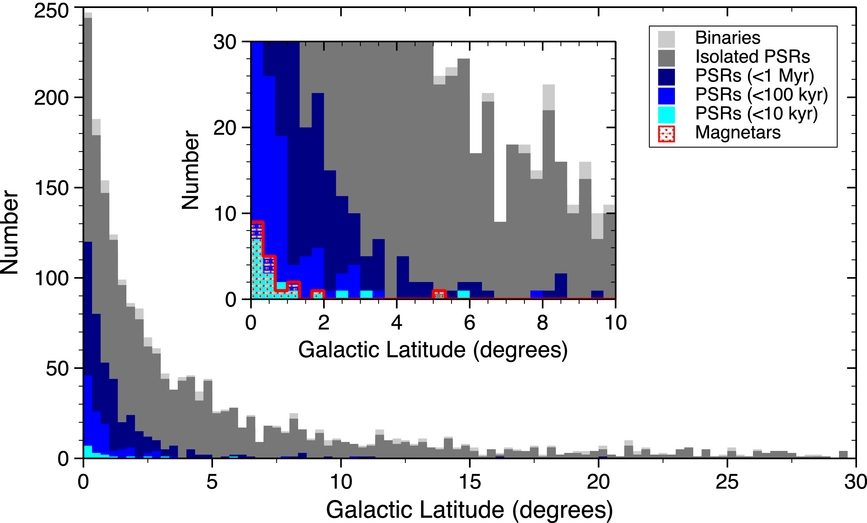
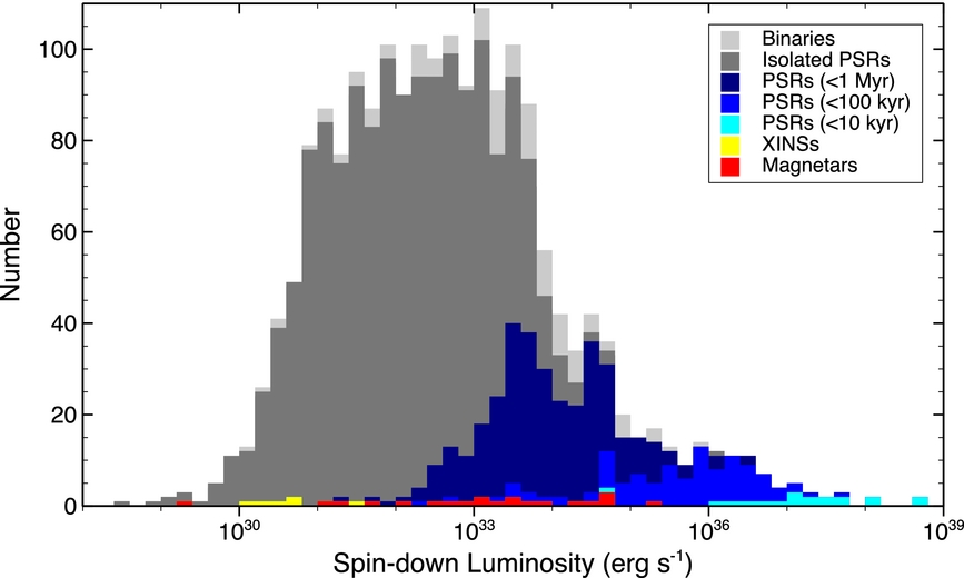
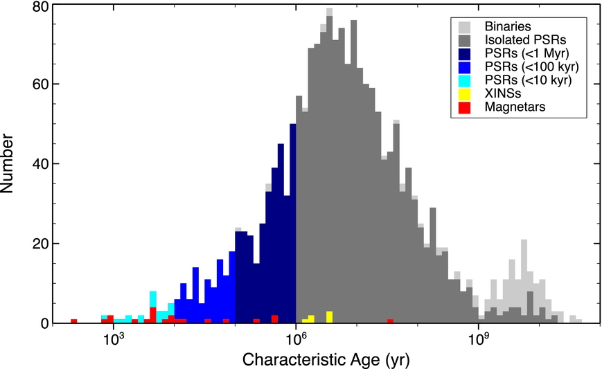
Figure 16. Magnetar detections as a function of quiescent 2–10 keV X-ray flux FX. Radio and hard X-ray detections are marked by red squares and blue circles, as described for Figure 15.
Download figure:
Standard image High-resolution image
The radio emission observed from magnetars is strikingly different from the hard X-ray behavior. As is clear from Figure 16, radio emission has only been seen in sources with low FX when in outburst in spite of extensive radio observations and stringent upper limits (see Table 5) of most of the objects cataloged including those with the largest values of FX (Burgay et al. 2006b; Crawford et al. 2007; Lazarus et al. 2012; Tong et al. 2013; Archibald et al. 2013).5 Although beaming may play a role (see discussion in Lazarus et al. 2012), with increasing statistics, the segregation of radio detections in the P– diagram (Figure 15) is interesting.
Rea et al. (2012b) have suggested that there exists a "fundamental plane" in magnetar spin and radiative phase space that distinguishes sources of different radio emission properties. Specifically, they argue on physical grounds that magnetars with high  and low LX should be radio bright, while low
  , high LX should not be radio detected. This is, in principle, an explanation for the striking asymmetry in the P–
 distribution we see for radio-emitting sources. On the other hand, the recent non-detection of magnetar Swift J1834.9−0846, which has
  where Rea et al. (2012b) would predict radio emission, argues against this picture (Tong et al. 2013; Esposito et al. 2013). Moreover, the "fundamental plane" picture also predicts radio emission from the high-B rotation-powered pulsar PSR J1846−0258, which in fact has been shown to be radio quiet (Archibald et al. 2008). Rea et al. (2012b) argue that a previously reported very large distance (21 kpc) to the source (Becker & Helfand 1984) together with its presence in supernova remnant Kes 75 could somehow hinder a radio detection, perhaps because of a high DM. However, up-to-date distance estimates for this pulsar (Leahy & Tian 2008a; Su et al. 2009) place it significantly closer (5.1–10.9 kpc), and the system's hydrogen column density as measured with X-ray observations, NH = 2–4 × 1022 cm−2 predicts, on the basis of an empirical DM versus NH law (He et al. 2013), DM ≃ 600–1300 pc cm−3. This is well within the range of observed DMs for radio pulsars, particularly those with only moderately fast rotation periods like the 0.326 s period of PSR J1846−0258. Hence, we disagree with the conclusion of Rea et al. (2012b) that a radio detection of PSR J1846−0258 is difficult due to its environment. On the other hand, unfortunate radio beaming, as well as the episodic nature of radio emission from magnetars, may play a role for this pulsar and Swift J1834.9−0846. Continued radio observations of magnetars in outburst to increase statistics for radio emission in the population will be helpful for deciding whether
  plays a meaningful role in radio detectability of magnetars.
4. CONCLUSIONS
We have compiled the first catalog of all currently known magnetars, including 21 confirmed sources and 5 candidates. Where available from the literature, we have provided spatial properties (coordinates, proper motion, distance, and proposed associations), timing data (period, period derivative, and derived parameters), spectral parameters for the quiescent soft X-ray emission, and observed properties or upper limits in the radio, infrared, optical, hard X-ray, and gamma-ray bands. We note that the known magnetar population is relatively free from selection for location in the Galaxy thanks to the all-sky X-ray monitors that have found so many of these objects in recent years. We constructed histograms in Galactic longitude and latitude, spin period, P, spin-inferred magnetic field, B, spin-down luminosity,  , and characteristic age, τc, to compare the magnetar distributions with the distributions of the known pulsar population. We measure the scale height of magnetars for the first time and find it to be smaller than that of OB stars, supporting the hypothesis that the most massive O stars are magnetar progenitors. We note the relatively narrow ranges in P and B observed for the magnetars, which stand in contrast to the far wider ranges in
  and τc. The fact that the characteristic age range is so broad, in spite of so small a scale height for these objects, argues that the former is generally a poor age indicator. We confirm correlations between Γ and B, previously identified by Kaspi & Boydstun (2010) and Enoto et al. (2010a), and LX and B, previously noted by An et al. (2012), and observe an excluded region in the plot of LX versus Γ. Finally, we find that detections of magnetars in the hard X-ray seem to be correlated with soft X-ray flux and B, while radio detections show, if anything, the opposite trend. A regularly maintained online version of the catalog has been made available, with one main table focused on the timing and X-ray data, and two additional tables for alternative values and detailed records of optical and near-infrared observations. We plan to maintain this with regular updates as new magnetar results appear and encourage the community to provide feedback and suggestions for improvement on this constantly evolving initiative.
We thank J. Lazio for assistance in producing Figure 2, as well as N. Murray, L. Drissen, J. Maíz Apellániz, C. Thompson, B. Gaensler, J. Halpern, S. Tendulkar, R. Duncan, and the McGill Pulsar Group for helpful discussions. We also thank K. Boydstun and C. Tam for their work on early versions of the online magnetar catalog, as well as the magnetar community for their past and continuing input. V.M.K. holds the Lorne Trottier Chair in Astrophysics and Cosmology as well as a Canada Research Chair, and acknowledges additional support from an NSERC Discovery Grant and Accelerator Supplement, from FQRNT via le Centre de Recherche Astrophysique du Québec and the Canadian Institute for Advanced Research.
APPENDIX A: MAGNETAR NAMES
In Table 8, we list the commonly used names (as well as a few less-common alternatives) of all cataloged magnetars along with our proposed new names. The names follow the convention MG JHHMM+/−DDMM (here, "MG" stands for "magnetar") similar to the naming convention for pulsars, and indeed, for the sake of comparison, we also list the PSR names used by the ATNF catalog in Table 8. Note that this naming scheme is only used for confirmed magnetars, though for completeness we also list the five magnetar candidates in the table.
APPENDIX B: ONLINE TABLES
The online version of the McGill Magnetar Catalog consists of three tables which summarize and expand upon some of the data presented in Section 2. The first of these tables is presented in Table 9. This is the main table of the online catalog and includes columns from Tables 1, 2, 3, and 7 in order to collect the timing and X-ray properties, distances, and positions of magnetars in one location. There are also columns to denote the wavebands for each magnetar at which persistent emission has been detected and the types of activity that have been observed. Table 10 shows the second of the online tables, which lists alternative published values for P and  , soft X-ray spectral parameters, and distance. On occasions where a magnetar was reported to have a widely varying
  over some period of time, the range of this variation is given in its own column. Further columns list, for observations where phase-resolved spectroscopy was performed, the range over which the spectral parameters varied in phase. The final table from the online catalog is given in Table 11. It tabulates individual observations of magnetars in the optical and near-infrared bands and can be considered an expansion of Table 4, with additional columns for the date of observation and any non-standard filters that were used. Tables 9–11 are available in their entirety in the electronic version of this article; for the most up-to-date versions see the online catalog.
Table 9. Main Table of the Online Catalog
| Name | P |  |
NH | Γ | kT | kT2 | Flux | Dist. | Opt/IRa | Bandsb | Activityc | R.A. | Decl. |
|---|---|---|---|---|---|---|---|---|---|---|---|---|---|
| CXOU J010043.1−721134 | 8.020392 | 1.88 | 0.063 | ... | 0.30 | 0.68 | 0.14 | 62.4 | Maybe | X | ... | 01 00 43.14 | −72 11 33.8 |
| 4U 0142+61 | 8.68832877 | 0.20332 | 1.00 | 3.88 | 0.410 | ... | 67.9 | 3.6 | Yes | HXOI | BG | 01 46 22.41 | +61 45 03.2 |
| SGR 0418+5729 | 9.07838822 | 0.0004 | 0.115 | ... | 0.32 | ... | 0.0020 | ∼2 | No | X | BT | 04 18 33.87 | +57 32 22.9 |
| SGR 0501+4516 | 5.76209653 | 0.582 | 0.6 | ... | 0.38 | ... | 0.83 | ∼2 | Yes | HXO | B | 05 01 06.76 | +45 16 33.9 |
| SGR 0526−66 | 8.0544 | 3.8 | 0.604 | 2.50 | 0.44 | ... | 0.55 | 53.6 | No | X | BF | 05 26 00.89 | −66 04 36.3 |
| 1E 1048.1−5937 | 6.4578754 | ∼2.25 | 0.97 | 3.14 | 0.56 | ... | 5.1 | 9.0 | Yes | HXO | BG | 10 50 07.14 | −59 53 21.4 |
| 1E 1547.0−5408 | 2.0721255 | ∼4.77 | 3.2 | 4.0 | 0.43 | ... | 0.54 | 4.5 | Maybe | HXR | BT | 15 50 54.12 | −54 18 24.1 |
| PSR J1622−4950 | 4.3261 | 1.7 | 5.4 | ... | 0.5 | ... | 0.045 | ∼9 | No | XR | ... | 16 22 44.89 | −49 50 52.7 |
| SGR 1627−41 | 2.594578 | 1.9 | 10 | 2.9 | ... | ... | 0.25 | 11.0 | No | X | BT | 16 35 51.84 | −47 35 23.3 |
| CXOU J164710.2−455216 | 10.610644 | <0.04 | 2.39 | 3.86 | 0.59 | ... | 0.25 | 3.9 | No | X | BT | 16 47 10.20 | −45 52 16.9 |
| 1RXS J170849.0−400910 | 11.003027 | 1.91 | 1.36 | 2.792 | 0.456 | ... | 24.3 | 3.8 | Maybe | HX | G | 17 08 46.87 | −40 08 52.4 |
| CXOU J171405.7−381031 | 3.825352 | 6.4 | 3.95 | 3.45 | ... | ... | 2.68 | ∼13.2 | No | X | ... | 17 14 05.74 | −38 10 30.9 |
| SGR J1745−2900 | 3.7635537 | 0.661 | ... | ... | ... | ... | <0.013 | ∼8.5 | No | HXR | BT | 17 45 40.16 | −29 00 29.8 |
| SGR 1806−20 | 7.547728 | ∼49.5 | 6.9 | 1.6 | 0.55 | ... | 18 | 8.7 | Yes | HXO | BF | 18 08 39.34 | −20 24 39.9 |
| XTE J1810−197 | 5.5403537 | 0.777 | 0.63 | ... | 0.18 | ... | 0.029 | 3.5 | Yes | XOR | BT | 18 09 51.09 | −19 43 51.9 |
| Swift J1822.3−1606 | 8.43771958 | 0.0306 | 0.453 | ... | 0.12 | ... | <0.025 | 1.6 | No | X | BT | 18 22 18.00 | −16 04 26.8 |
| SGR 1833−0832 | 7.5654084 | 0.35 | ... | ... | ... | ... | <0.2 | ... | No | X | B | 18 33 44.37 | −08 31 07.5 |
| Swift J1834.9−0846 | 2.4823018 | 0.796 | ... | ... | ... | ... | <0.004 | 4.2 | No | X | BT | 18 34 52.12 | −08 45 56.0 |
| 1E 1841−045 | 11.782898 | 3.93 | 2.2 | 1.9 | 0.45 | ... | 21.3 | 8.5 | Maybe | HX | BG | 18 41 19.34 | −04 56 11.2 |
| SGR 1900+14 | 5.19987 | 9.2 | 2.12 | 1.9 | 0.47 | ... | 4.8 | 12.5 | Maybe | HX | BF | 19 07 14.33 | +09 19 20.1 |
| 1E 2259+586 | 6.978948446 | 0.04843 | 1.012 | 3.75 | 0.37 | ... | 14.1 | 3.2 | Yes | HXOI | BGA | 23 01 08.30 | +58 52 44.5 |
| SGR 1801−23 | ... | ... | ... | ... | ... | ... | ... | ... | No | ... | B | 18 00 59 | −22 56 48 |
| SGR 1808−20 | ... | ... | ... | ... | ... | ... | ... | ... | No | ... | B | 18 08 11.2 | −20 38 49 |
| AX J1818.8−1559 | ... | ... | 3.6 | 1.17 | ... | ... | 1.68 | ... | No | X | B | 18 18 51.38 | −15 59 22.6 |
| AX J1845.0−0258 | 6.97127 | ... | 7.8 | 1.0 | ... | ... | 0.33 | ∼8.5 | No | X | T | 18 44 54.68 | −02 56 53.1 |
| SGR 2013+34 | ... | ... | ... | ... | ... | ... | ... | ∼8.8 | No | ... | B | 20 13 56.9 | +34 19 48 |
Notes. aWhether or not an optical/near-infrared counterpart has been identified. bWavebands in which persistent emission has been detected. H: soft gamma-rays/hard X-rays (>10 keV), X: X-rays (1–10 keV), O: optical/near-infrared, I: mid- to far-infrared, R: radio. cB: bursts, F: giant flare, G: glitch, A: anti-glitch, T: transient magnetar.
Only a portion of this table is shown here to demonstrate its form and content. A machine-readable version of the full table is available.
Download table as: DataTypeset image
Table 10. Variable or Alternative Values
| Name | P |  |
 Rangea Rangea |
NH | NH Rangeb | Γ | Γ Rangeb | kT | kT Rangeb | kT2 | Flux | Distance |
|---|---|---|---|---|---|---|---|---|---|---|---|---|
| 1E 1547.0−5408 | 2.06983302 | 2.318 | ... | 3.1 | ... | 3.7 | ... | 0.43 | ... | ... | 0.44 | 9 |
| ... | ... | 2.35–3.16 | 3.2 | ... | 4.0 | ... | 0.43 | ... | ... | 0.54 | 4.5 | |
| 2.0721255 | 4.77 | 2.66–9.78 | ... | ... | ... | ... | ... | ... | ... | ... | ... | |
| 1RXS J170849.0−400910 | ... | ... | ... | 1.42 | 1.0–2.0 | 2.62 | 1.90–3.15 | 0.46 | 0.380–0.535 | ... | 42.1 | ... |
| ... | ... | ... | 1.36 | 1.1–1.6 | 2.40 | 2.0–2.9 | 0.44 | 0.42–0.49 | ... | 69.4 | ... | |
| ... | ... | ... | 1.36 | 1.28–1.66 | 2.83 | 2.2–3.2 | 0.456 | 0.35–0.52 | ... | 24.5 | ... | |
| ... | ... | ... | 1.36 | ... | 2.74 | ... | 0.42 | ... | ... | 36.8 | ... | |
| ... | ... | ... | 1.36 | ... | 2.792 | ... | 0.456 | ... | ... | 24.3 | ... | |
| XTE J1810−197 | 5.5403537 | 0.777 | 0.430–1.04 | 0.63 | ... | ... | ... | 0.18 | ... | ... | 0.030 | 3.3 |
| ... | ... | ... | 0.63 | ... | ... | ... | 0.19 | ... | ... | ... | 3.1 | |
| ... | ... | ... | 0.60 | ... | ... | ... | 0.167 | ... | 0.33 | ... | 3.5 | |
| ... | ... | ... | 0.72 | ... | ... | ... | 0.144 | ... | 0.301 | ... | ... | |
| Swift J1822.3−1606 | 8.43772016 | 0.0083 | ... | <0.7 | ... | ... | ... | 0.20 | ... | ... | <0.025 | ... |
| 8.43771958 | 0.0306 | ... | 0.453 | ... | ... | ... | 0.12 | ... | ... | <0.0013 | ... |
Notes.
aIn cases where a source was reported to have a widely varying  over a period of time, the range over which
  varied is given here.
bFor observations where phase-resolved spectroscopy was performed, the range over which the parameter varied in phase is given here.
varied is given here.
bFor observations where phase-resolved spectroscopy was performed, the range over which the parameter varied in phase is given here.
Only a portion of this table is shown here to demonstrate its form and content. A machine-readable version of the full table is available.
Download table as: DataTypeset image
Table 11. Optical/Near-infrared Counterparts
| Name | ObsDate | Ks | H | J | I | R | V | B | U |
|---|---|---|---|---|---|---|---|---|---|
| SGR 0501+4516 | 2008 Aug 22 | K = 18.6 | ... | ... | ... | ... | ... | ... | ... |
| 2008 Aug 24 | ... | ... | ... | ... | >23.0 | ... | ... | ... | |
| 2008 Aug 25 | 19.2 | ... | ... | ... | ... | ... | ... | ... | |
| 2008 Aug 25 | ... | ... | ... | 23.3 | ... | ... | ... | ... | |
| 2009 Jan 1 | ... | ... | ... | i' = 24.4 | ... | ... | g' > 26.9 | u' > 24.7 | |
| 2009 Jan 28 | K = 19.7 | ... | ... | ... | ... | ... | ... | ... | |
| 1E 1547.0−5408 | 2007 Jul 12 | >21.7 | ... | ... | ... | ... | ... | ... | ... |
| 2008 Oct 3 | ... | ... | ... | ... | ... | >20.4 | >20.7 | >20.3 | |
| 2009 Jan 18 | >20.1 | ... | ... | ... | ... | ... | ... | ... | |
| 2009 Jan 24 | 18.5 | ... | ... | ... | ... | ... | ... | ... | |
| Swift J1822.3−1606 | 2006 May 3 | K > 17.3 | >18.3 | >19.3 | ... | ... | ... | ... | ... |
| 2011 Jul 21 | ... | ... | ... | z > 22.2 | ... | ... | ... | ... | |
| SGR 1833−0832 | 2010 Mar 19 | ... | ... | ... | ... | ... | >21.4 | >21.3 | >22.3 |
| 2010 Mar 20 | ... | ... | ... | z' > 24.9 | ... | ... | ... | ... | |
| 2010 Mar 25 | >22.4 | ... | ... | ... | ... | ... | ... | ... |
Only a portion of this table is shown here to demonstrate its form and content. A machine-readable version of the full table is available.
Download table as: DataTypeset image
Footnotes
- *
An online version of the catalog is located at http://www.physics.mcgill.ca/~pulsar/magnetar/main.html.
- 1
- 2
- 3
- 4
http://www.atnf.csiro.au/research/pulsar/psrcat/, version 1.47
- 5
We note the claimed radio detections of 4U 0142+61, 1E 2259+586, and XTE J1810−197 (Malofeev et al. 2012); however, the detections have not yet been confirmed using another observatory.