

Abstract
3D non-linear MHD simulations of a D2 massive gas injection (MGI) triggered disruption in JET with the JOREK code provide results which are qualitatively consistent with experimental observations and shed light on the physics at play. In particular, it is observed that the gas destabilizes a large m/n = 2/1 tearing mode, with the island O-point coinciding with the gas deposition region, by enhancing the plasma resistivity via cooling. When the 2/1 island gets so large that its inner side reaches the q = 3/2 surface, a 3/2 tearing mode grows. Simulations suggest that this is due to a steepening of the current profile right inside q = 3/2. Magnetic field stochastization over a large fraction of the minor radius as well as the growth of higher n modes ensue rapidly, leading to the thermal quench (TQ). The role of the 1/1 internal kink mode is discussed. An Ip spike at the TQ is obtained in the simulations but with a smaller amplitude than in the experiment. Possible reasons are discussed.
Export citation and abstract BibTeX RIS
1. Introduction
In order to develop a predictive modelling capability in support of the design and operation of the ITER disruption mitigation system (DMS) [1, 2], it is essential to validate models on present devices as well as to understand the physical mechanisms at play. The present paper describes progress made with the JOREK 3D non-linear magnetohydrodynamics (MHD) code in the domain of massive gas injection (MGI), one of the options considered for the ITER DMS. The focus is put on the pre-thermal quench (TQ) and TQ phases. The current quench (CQ) phase will be the object of future work.
A publication by Fil et al in 2015 [3] introduced first results from simulations of a pure D2 MGI into a JET Ohmic plasma. Work has been pursued since then on the same case and with essentially the same model, but with more realistic input parameters thanks to numerical improvements. This has lead to significant progress which is presented in this paper. Most notably, while only an incomplete TQ was obtained in [3], simulations now display a more proper TQ. Furthermore, numerical experiments as well as a detailed analysis of simulation results have led to a better understanding of the physics at play.
The paper is constructed as follows. In section 2, the experiment is introduced. Section 3 presents the model and section 4 the setup of simulation parameters, highlighting differences with [3]. Section 5 gives an overview of a simulation, after which sections 6 and 7 describe investigations on the mechanisms at play during the pre-TQ and TQ phases, respectively. Finally, section 8 concludes.
2. The experiment
The modelled case has already been described in the paper by Fil et al [3] but it is briefly described again here for convenience. This is JET pulse 86887, an Ohmic pulse with  T,
T,  MA, q95 = 2.9 in which a disruption was MGI-triggered on a 'healthy' plasma by activating the disruption mitigation valve number 2 (DMV2) pre-loaded with D2 at 5 bar. The gas is injected at the outer midplane. Central values of the electron density and temperature prior to the MGI are
  m−3 and
  keV. The volume of the DMV2 reservoir is 10−3 m3 and its temperature is about 300 K, so it initially contains about
  D2 molecules, which represents roughly 100 times more D nuclei than initially present in the plasma.
Figure 1 shows an overview of the disruption phase. First effects of the MGI are visible from about 2 ms (relative to the DMV2 trigger) in the form of increases in the line integrated density and radiated power. The TQ occurs at about 12 ms as can be seen from the fast collapse of the central soft x-ray (SXR) signal accompanied by a burst of MHD activity and immediately followed by the characteristic Ip spike. The CQ ensues.

Figure 1. Experimental time traces for JET pulse 86887, from top to bottom: plasma current Ip, magnetic fluctuations from Mirnov coil, radiated power from bolometry, line integrated density from interferometry, and soft x-rays signal from a central chord. The time origin corresponds to the DMV2 trigger.
Download figure:
Standard image High-resolution image3. The model
The model used here is essentially the same as in [3] (with only a few differences detailed below). The reader is therefore referred to [3] for a more complete model description. Nevertheless, for convenience we write again the equations here:


ψ is the poloidal flux,  the toroidal current density times the major radius, u the poloidal flow potential, ω the toroidal vorticity, ρ the plasma mass density, T the total (ion + electron) temperature,
  the parallel (to the magnetic field) velocity and
  the neutral mass density. Sion and
  designate respectively the ionization and recombination rate coefficients for deuterium, parameterized as detailed in [3]. Note that apart from the neutral source, there are no sources in the model. Realistic sources indeed have a negligible effect on the small timescale of the disruption. Hyper-resistivity/conductivity/viscosity terms, not shown above, are also included for numerical stability reasons.
There are two differences between the present model and that of [3]. First, for the sake of energy conservation, the resistivity used in the Ohmic heating term of equation (6) is the same as in equation (1), while in [3] the Spitzer resistivity was used. Second, D radiation terms have been suppressed for simplicity after verifying that they do not influence the results significantly.
4. Simulations setup
4.1. Initial conditions and general parameters
Initial density and temperature profiles are taken from Thomson scattering measurements, asssuming  . The initial magnetic equilibrium is calculated from EFIT data as explained in [3]. Toroidal rotation is initialized at 0. Table 1 gives the value of input parameters used here as well as in [3]. Improvements in the poloidal mesh now allow running simulations with a hyper-resistivity
  and hyper-viscosity
  roughly 500 times smaller than in [3], which removes the artificial stabilization of the MHD activity due to these coefficients in [3]. Also, present simulations use much smaller diffusion coefficients than in [3], both for ions/electrons and for neutrals. The artificial core dillution observed in [3] is therefore not present anymore. It is important to recall that realistic temperature dependencies are used for the resistivity and parallel thermal conductivity:
  and
and  , where T0 is the initial temperature at the center of the plasma. For
  , the Spitzer–Härm value is used, while
  is typically one order of magnitude larger than the Spitzer value.
Table 1. List of typical values of JOREK input parameters used in the present paper as well as in [3].
| Parameter | Symbol | Value in present paper | Value from [3] | Units | Comment |
|---|---|---|---|---|---|
| Initial central resistivity |  |
 – – |
Same | SI ( ) ) |
Spitzer value:  |
| Resistive time at q = 2 |  |
4 − 0.4 | Same | SI (s) | Exp. value: 7 |
| Lundquist number at q = 2 |  |
 – – |
Same | Adimensional | Exp. value:  |
| Hyper-resistivity |  |
 |
 |
JOREK | |
| Initial central // thermal conductivity |  |
 |
 |
SI ( ) ) |
Spitzer–Härm value:  |
 thermal conductivity thermal conductivity |
 |
 |
Same | SI ( ) ) |
Corresponds to  m2 s−1 m2 s−1 |
Hyper- thermal conductivity thermal conductivity |
 |
10−12 | Same | JOREK | |
| Dynamic viscosity | μ |  |
 |
SI (kg/m/s) | Corresponds to  m2 s−1 m2 s−1 |
| Hyper-viscosity |  |
 |
 |
JOREK | |
| // viscosity |  |
 |
 |
SI (kg/m/s) | Corresponds to  m2 s−1 m2 s−1 |
| Hyper-// viscosity |  |
10−9 | Same | JOREK | |
Ion/electron particle  diffusivity diffusivity |
 |
1.4 | 28 | SI (m2 s−1) | |
| Ion/electron particle // diffusivity |  |
0 |  |
SI (m2 s−1) | |
| Neutral particle diffusivity | Dn | 60–6000 |  |
SI (m2 s−1) |
4.2. Gas source setting
The physics of gas penetration into the plasma during an MGI is rather complex [4] and it is clear that the present model is not appropriate to describe it accurately. In other terms, JOREK simulations are not predictive in this respect. The gas source is therefore adjusted so as to best match interferometry data. Its temporal shape is based on the solution for the gas flow in vacuum [3] but using a DMV2 pressure of 0.1 bar instead of the experimental 5 bar (which can be interpreted as a sign of the low fuelling efficiency of the MGI). Note that in [3], a much larger value of typically 1 bar was needed due to the use of much larger particle diffusion coefficients. The gas source is located at the edge of the plasma (centered 5 cm inside the separatrix) and localised both poloidally and toroidally (see [3] for precisions). Figure 2 shows experimental and synthetic line integrated densities nel for three interferometry lines of sight (LoS). Three simulations are shown, with different toroidal localisations of the source:  (dashed), 2 (plain) and 100 (i.e. virtually axisymmetric, dash-dotted) respectively (angles are given in radians). Even though the same number of neutrals is injected in each simulation, clear differences appear in the synthetic nel. In order to interprete these differences, one should consider that interferometry chords are located 180 degrees away toroidally from DMV2, as shown in figure 3. Poloidal cross-sections of ne in the interferometer plane are shown in figure 4 for
  (top) and
  (bottom). These figures indicate that LoS 2 (red) runs through a region which is connected to the gas deposition region and therefore sees a faster increase in nel than LoS 3 (blue) for
  (dashed) but not for
  (dash-dotted). The simulation at
  actually matches experimental data very well for the three LoS until about 3 ms, after which the agreement deteriorates for a yet unidentified reason. Over a larger period of time, the case
  is the one that offers the best global match and is therefore selected for a detailed description and analysis below.

Figure 2. Time evolution of the measured (circles) and simulated (lines—plain =  ; dashed =
  ; dash-dotted =
  ) line integrated density for the three interferometry lines of sight.
Download figure:
Standard image High-resolution image
Figure 3. Schematic machine view from the top showing the DMV2 and interferometer chords.
Download figure:
Standard image High-resolution image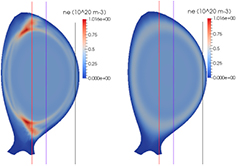
Figure 4. Poloidal cross-sections of ne in the plane of the interferometer as simulated with JOREK for  (left) and
  (right). Interferometry chords are also shown, with the same color code as in figure 2.
Download figure:
Standard image High-resolution image5. Overview of a simulation
Snapshots of the above simulation with  are shown in figure 5. For a series of times through the simulation (different rows), poloidal cross sections of (from left to right) Te, ne,
  as well as a Poincaré plot are shown. The top row shows the initial state. The second row shows the situation at t = 4.1 ms, during the pre-TQ phase. It can be seen that the gas has increased ne and decreased Te at the edge of the plasma and given birth to an m/n = 2/1 magnetic island, clearly visible on the Poincaré plot and whose effect on Te, ne and
  is also clear. The island O-point coincides with the gas deposition region, which is in line with experimental observations for Ohmic plasmas in JET [5] (we will come back to this point in section 6). A 1/1 island is also visible in the core which indicates the growth of an internal kink mode (q0 < 1 in this simulation, consistently with the presence of sawteeth in this pulse). In the third row, at t = 5.7 ms, the magnetic field has become stochastic over roughly the outer half of the plasma, which leads to a temperature flattening by parallel conduction in this region. However, the core is still hot at this stage. Finally, at t = 6.2 ms (fourth row), the core Te has collapsed via a convective mixing related to the 1/1 mode. The behaviour observed in this simulation is similar to the one found in NIMROD simulations for other tokamaks [6, 7].

Figure 5. Poloidal cross sections at the toroidal position of the MGI of (from left to right) Te, ne,  and Poincaré plots at times (from top to bottom) t = 0, t = 4.1 ms, t = 5.7 ms and t = 6.2 ms.
Download figure:
Standard image High-resolution image6. Physics of the pre-thermal quench phase
Let us now analyse the mechanisms at play, beginning with the pre-TQ phase. An important question is how the gas generates the 2/1 tearing mode. One may imagine at least three possible mechanisms. The first one is that the gas creates a 3D pressure field to which  and
and  have to adjust in order for force balance to pertain, leading to a 3D equilibrium which may imply a 2/1 tearing mode. The other two mechanisms, in contrast to the first one, are directly related to the temperature dependence of the resistivity η. One is an axisymmetric effect: the gas cools the edge of the plasma, increasing η and therefore contracting the current profile. This should increase the current density gradient
  at the edge of the still hot region. When the steep gradient gets just inside the q = 2 surface, the 2/1 tearing mode should be destabilized via the following term in the resistive MHD energy principle [8]:
  . The other η-related effect is a non-axisymmetric one: the gas cools the plasma locally and therefore suppresses the current locally, which should lead to the growth of magnetic islands with their O-point at the gas deposition location. This mechanism is involved as well in radiation driven islands, which have been invoked recently to explain density limit disruptions [9]. To a certain extent, numerical experiments allow discriminating between the three above-mentioned mechanisms. Figure 6 shows the evolution of the magnetic energy contained in the n = 1 toroidal harmonic for three simulations. In the first one (blue), the standard
  dependence was used. In the second one (red), we used instead
  , where Tn=0 is the axisymmetric component of T, in order to suppress the non-axisymmetric η-related mechanism. Finally, in the third simulation (black), the T dependence of η was removed altogether by keeping the initial η profile, in order to remove both η-related effects. All three simulations are overimposed until about 0.5 ms, indicating that the early evolution is not η-related and therefore likely connected to the 3D equilibrium mechanism. However, in the third (black) simulation the n = 1 magnetic energy quickly saturates and the 2/1 island remains very small. The leading mechanisms for the 2/1 island growth are therefore η-related, even if the island grows from a non-η-related seed. Then, it appears that between 0.5 and 2.5 ms, the
  case gains about one order of magnitude compared to the
  case, showing that the non-axisymmetric η-related effect is important. This is consistent with the already mentioned experimental observation that the island O-point coincides with the gas deposition region for Ohmic plasmas [5]. Note that for neutral beam heated plasmas, the alignment is observed to degrade [5], which may be due to plasma rotation via two effects: a smearing of the non-axisymmetric η-related effect and a drag of the island into the plasma flow.

Figure 6. Time evolution of the magnetic energy contained in the n = 1 component for three simulations with different models for the resistivity (see text).
Download figure:
Standard image High-resolution image7. Physics of the thermal quench
7.1. Triggering of the thermal quench
The next question is: what mechanisms trigger the TQ? This question may be addressed by analysing figures 7 and 8. Figure 7 shows the time evolution of the magnetic energy in the different toroidal harmonics (note the logarithmic vertical scale). Figure 8 contains poloidal cross-sections of the cosine component of ψ for the n = 1 (left), n = 2 (middle) and n = 3 (right) harmonics at different times (different rows). Both figures are for the same simulation as in section 5. It can be seen in figure 7 that during the first 5 ms, magnetic perturbations are strongly dominated by the n = 1 mode. The top left plot of figure 8 shows that the mode has a 2/1 structure, not surprisingly. Then, at about 5 ms, a clear increase in the growth rate of the n = 2 magnetic energy is visible. This is associated to the growth of a 3/2 tearing mode, as can be seen by comparing the first and second rows, middle column, plots in figure 8. Around 5.8 ms, magnetic energies in higher n harmonics grow sharply. For example, a 4/3 mode can be seen to grow when comparing the second and third rows, last column, plots in figure 8. This leads to the TQ.
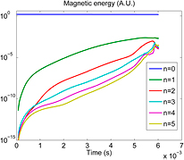
Figure 7. Time evolution of the magnetic energy in the different toroidal harmonics.
Download figure:
Standard image High-resolution image
Figure 8. Poloidal cross-sections at the toroidal position of the MGI of (from left to right) the n = 1, n = 2 and n = 3 cosine component of ψ at times (from top to bottom) t = 4.1 ms, t = 5.1 ms and t = 5.7 ms (same simulation as in figures 5, 7 and 9). The color scale is the same for all plots (note the saturation for the n = 1 mode which has a large amplitude compared to the other modes).
Download figure:
Standard image High-resolution imageMechanisms for the growth of the 2/1 mode have been discussed in section 6. What about the other modes? Looking at Poincaré plots, it appears that the 3/2 mode starts growing when the inner side of the 2/1 island reaches the q = 3/2 surface. Observing the  profile at different times, shown in figure 9, it seems likely that this is due to a current profile effect. Indeed, the 2/1 island causes a local
  flattening, which steepens the profile radially inward (compare the black, blue and red profiles). The 3/2 mode grows when the large
  region runs across the q = 3/2 surface (i.e. between the blue and red profiles) due to the
  term in the energy principle already mentioned in section 6. The same process then seems to take place with the 3/2 tearing mode, which locally flattens
  (red versus magenta profiles), moving the large
  region across q = 4/3 and destabilizing the 4/3 mode. Therefore, it seems that the TQ is triggered by a kind of current profile avalanche. Note that this picture for the TQ triggering has already been proposed in [6] and [8]. The magnetic stochasticity created by the tearing modes in (roughly) the outer half of the plasma flattens the temperature profile there. In this simulation, flux surfaces however pertain inside mid-radius so that the central temperature cannot collapse purely from parallel thermal conduction. Convective core mixing indeed seems to play an important role in this simulation. However, as we shall see below, it is likely that tearing modes are too weak in this simulation. In other simulations where the tearing modes were excited more strongly (due to different MGI settings for example), magnetic stochasticity extended across the whole plasma. Hence, convective core mixing and the 1/1 internal kink mode may not play a large role in reality, but this is not clear at this stage.
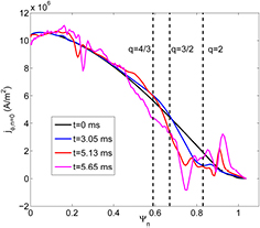
Figure 9. Toroidal current density profiles at the midplane (low field side) at different times. Note that the red and magenta profiles correspond to the last two rows of figure 8.
Download figure:
Standard image High-resolution image7.2. The plasma current spike
The Ip spike is a characteristic feature of disruptions. A classic explanation of its origin is that the TQ releases magnetic energy  (where li is the internal inductance of the plasma) while the flux ψ at the edge of the plasma does not have the time to change significantly because the TQ is much shorter than the wall penetration time, and hence
  should remain constant, where
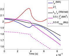
 ![${{L}_{\text{p}}}\simeq {{\mu}_{0}}R\left[\ln (8R/a)-2+{{l}_{\text{i}}}/2\right]$](https://content.cld.iop.org/journals/0741-3335/59/1/014006/revision1/ppcfaa3c04ieqn090.gif) is the self-inductance of the plasma. The consequence is that li has to decrease and Ip increase, hence the Ip spike. JOREK results are well in line with this explanation, as seen in figure 10, which displays the evolution of Ip, li, the magnetic energy inside the plasma (Emag and its approximation
is the self-inductance of the plasma. The consequence is that li has to decrease and Ip increase, hence the Ip spike. JOREK results are well in line with this explanation, as seen in figure 10, which displays the evolution of Ip, li, the magnetic energy inside the plasma (Emag and its approximation  ) and
) and  (for a different simulation from above because the latter has a smaller Ip spike). The fact that simulations display an Ip spike in spite of having no sources answers a criticism made by Zakharov to NIMROD simulations [10, 11]. The simulated Ip spike is however much smaller than the experimental one (compare figures 10 and 1). Following the above argument, this should mean that not enough magnetic energy is released during the TQ and that li does not decrease enough, i.e. that the current profile avalanche is not sufficiently pronounced. The strength of the avalanche may be expected to have a positive dependence on the ratio between the resistive diffusion time and the growth time of the 2/1 mode: indeed, the larger this ratio, the larger the current gradient inside the 2/1 island, and the stronger the excitation of inner modes. A stronger local cooling near q = 2 should go in this direction. The above simulation may therefore have a too weak cooling. This is also consistent with the fact that simulations over-predict the pre-TQ duration when appproaching a realistic η value. It is plausible that background impurities such as Argon remaining from previous pulses (where Ar MGI was used) [12] provide this extra cooling. The need for background impurities to match experimental observations had already been identified for He MGI simulations in Alcator C-Mod and DIII-D with NIMROD [7].
Figure 10. Time traces (from a different simulation than figures 5, 7–9, in which the Ip spike is smaller) showing an Ip spike at the TQ (blue curve) with  remaining approximately constant (black curve) while the current profile flattens (red curve) and magnetic energy is dissipated (magenta curves).
Download figure:
Standard image High-resolution image
8. Conclusion
JOREK simulations shed light on the physics of the pre-TQ and TQ phases of a D2 MGI-triggered disruption in an Ohmic JET plasma. The gas destabilizes (essentially via increasing η by cooling) a 2/1 tearing mode which flattens the current profile, destabilizing a 3/2 mode, which in turn destabilizes higher n modes. The energy is lost by parallel conduction along stochastic field lines and possibly also by a convective mixing of the core, but this will have to be clarified in the future. Indeed, the Ip spike in the simulations is too weak, suggesting that tearing modes are not large enough, and simulations with larger tearing modes (which display a larger Ip spike) produce a full stochastization of the magnetic field so that the convective core mixing plays a less important role. An interesting question which could be the object of future work is whether the TQ triggering picture found here may explain the experimental finding that the TQ is triggered at a distinct locked mode amplitude [13]. The work with JOREK on D2 MGI simulations shall in any case be pursued, aiming for quantitative validation. For this purpose, the effect of background impurities (as well as toroidal rotation, diamagnetic effects, etc) shall be investigated and efforts made to approach realistic parameter values, in particular for η. D2 MGI ASDEX Upgrade simulations have been begun, for which it is easier to run at realistic parameter values. In parallel to this work, a model for MGI of other gases than D2 has been implemented in JOREK and shall be utilized in the near future.
Acknowledgments
This work has been carried out within the framework of the EUROfusion Consortium and has received funding from the Euratom research and training programme 2014–2018 under grant agreement No 633053. The views and opinions expressed herein do not necessarily reflect those of the European Commission. This work was granted access to the HPC resources of Aix-Marseille University financed by the project Equip@Meso (ANR-10-EQPX-29-01). A part of this work was carried out using the HELIOS supercomputer system (IFERC-CSC), Aomori, Japan, under the Broader Approach collaboration, implemented by Fusion for Energy and JAEA, and using the CURIE supercomputer, operated into the TGCC by CEA, France, in the framework of GENCI and PRACE projects.