Abstract
Ultracold atomic gases provide a novel platform with which to study spin–orbit coupling, a mechanism that plays a central role in the nuclear shell model, atomic fine structure and two-dimensional electron gases. This paper introduces a theoretical framework that allows for the efficient determination of the eigenenergies and eigenstates of a harmonically trapped two-atom system with short-range interaction subject to an equal mixture of Rashba and Dresselhaus spin–orbit coupling created through Raman coupling of atomic hyperfine states. Energy spectra for experimentally relevant parameter combinations are presented and future extensions of the approach are discussed.
Export citation and abstract BibTeX RIS

Content from this work may be used under the terms of the Creative Commons Attribution 3.0 licence. Any further distribution of this work must maintain attribution to the author(s) and the title of the work, journal citation and DOI.
Over the past decade, much progress has been made in preparing isolated ultracold few-atom systems experimentally [1–4]. Moreover, a variety of tools for manipulating and probing such systems have been developed. On the theoretical side, a number of analytical and numerical approaches have been developed [5–13]. A large number of analytical treatments approximate the true alkali atom–alkali atom potential by a zero-range potential [8, 14–16]. This replacement yields reliable results in the low-energy regime where the de Broglie wave length is larger than the van der Waals length. For example, using zero-range contact interactions, the energy spectrum of two harmonically trapped atoms has been determined analytically [8–10]. These two-body solutions are available in 1D, 2D and 3D [8], and have played a vital role in guiding and interpreting experiments [17–19] as well as in theoretical studies of the two-body dynamics [20, 21] and of larger harmonically trapped systems [11–13, 22–24].
Recently, synthetic gauge fields, which allow for the realization of Hamiltonians that contain spin–orbit coupling terms, have been realized experimentally [25–35]. The purpose of this paper is to address how the trapped two-particle spectrum, obtained by modeling the two-body interaction via a zero-range δ-function, changes in the presence of spin–orbit and Raman coupling. While the two-particle system with spin–orbit coupling in free space [36–39] as well as the trapped single-particle system with spin–orbit coupling [40, 41] have received considerable attention, little is known about the trapped two-particle system with spin–orbit coupling and two-body interaction [42, 43]. In going from the trapped single-atom to the trapped two-atom system, a new length scale, i.e., the atom–atom scattering length, comes into play. Thus, an interesting question concerns the interplay between the interaction energy and the energy scales associated with the spin–orbit and Raman coupling strengths.
Our framework applies to the situation where the spin–orbit (or more precisely, spin–momentum) coupling term acts, as in recent experiments [29–35], along one spatial direction, say the x-direction. This corresponds to an equal mixture of Rashba and Dresselhaus spin–orbit coupling [44, 45]. For simplicity, we assume that the harmonic confinement in the other two spatial directions is much larger than that in the direction where the spin–orbit coupling term acts. This assumption reduces the problem to an effective one-dimensional Hamiltonian in the x-coordinates with effective 1D two-body interaction. The relationship between the true 3D atom–atom and effective 1D atom–atom interaction has been derived in [46–48]. We find analytical solutions to the two-atom system for arbitrary spin–orbit coupling strength and scattering length and vanishing Raman coupling strength. The case of non-zero Raman coupling strength is treated by expressing the system Hamiltonian in terms of the eigenstates for vanishing Raman coupling strength. We find that the relevant Hamiltonian matrix elements have closed analytical expressions, leaving the matrix diagonalization as the only numerical step. The developed framework can, as discussed toward the end of our paper, be readily generalized to a spherically-symmetric harmonic trap or an axisymmetric trap. Moreover, the framework developed also lays the groundwork for treating dynamical aspects of trapped two-body systems with non-vanishing spin–orbit and Raman coupling strengths and for treating the corresponding three-body system.
We consider two structureless one-dimensional particles of mass m subject to a single-particle spin–orbit coupling term with strength  , a Raman coupling term with strength Ω, detuning δ, and an external harmonic potential with angular trapping frequency ω. For
  , the two-particle Hamiltonian is given by
  ,
,
where xj
denotes the position coordinate of the jth particle and  the short-range interaction potential. For non-zero
  , Ω and δ, the two-particle Hamiltonian is given by H,
where  and
and  denote Pauli matrices,
  the identity matrix and pxj
the momentum of the jth particle. In the following, we first derive solutions to the time-independent Schrödinger equation governed by H with
the identity matrix and pxj
the momentum of the jth particle. In the following, we first derive solutions to the time-independent Schrödinger equation governed by H with  and then discuss how to obtain the solutions for non-zero Ω.
To determine the eigenstates and eigenenergies of H, we perform a rotation in spin space [49]. Specifically, we define  via a unitary transformation of H,
  , where
 ![$U={\rm exp} [\imath (\sigma _{x}^{(1)}+\sigma _{x}^{(2)})\pi /4]$](https://content.cld.iop.org/journals/0953-4075/47/16/161001/revision1/jpb498910ieqn12.gif) . The eigenenergies of the Hamiltonian H and
. The eigenenergies of the Hamiltonian H and  coincide while the eigenstates Ψ of the Hamiltonian H are related to the eigenstates
  of the Hamiltonian
  through
  . A straightforward calculation shows that
  and
and  for q = x and y, respectively. Correspondingly, we have
For  ,
,  is diagonal in the pseudo-spin basis
  ,
,  ,
,  and
and  with diagonal elements
  ,
,  ,
,  and
and  . To find the corresponding eigenstates, we approximate the two-body interaction by a delta-function interaction with coupling constant g,
  . For this interaction model, the eigenenergies and eigenstates of
  are known in compact form [8]. States that are even in the relative coordinate are affected by the coupling constant g while those that are odd in the relative coordinate are not. For states that are even in the relative coordinate, the eigenenergies
  of
of  (see solid lines in figure 1 for the n = 0 energies) are given by
  , where the center of mass quantum number n takes the values
  and the non-integer quantum number q is determined by the transcendental equation [8]

here,  denotes the harmonic oscillator length,
  . The corresponding eigenfunctions
  are given by
  , where the relative and center of mass coordinates are defined through
  and
and  , respectively. The relative wave functions
  can be written in terms of the confluent hypergeometric function U [8],

where Nq
denotes a normalization constant. The center of mass functions  are given by the one-dimensional harmonic oscillator functions for a mass m particle,
 ![${{\Phi }_{n}}(X)=N_{n}^{{\rm ni}}{{H}_{n}}(X/{{a}_{{\rm ho}}}){\rm exp} [-{{X}^{2}}/(2a_{{\rm ho}}^{2})]$](https://content.cld.iop.org/journals/0953-4075/47/16/161001/revision1/jpb498910ieqn44.gif) , where Hn
denotes the Hermite polynomial of order n and
, where Hn
denotes the Hermite polynomial of order n and  . For states that are odd in the relative coordinate, the eigenenergies
  of
of  (see dotted lines in figure 1 for the n = 0 energies) are given by
  , where q and n take the values
  . In this case, the eigenfunctions
  are simply products of the non-interacting harmonic oscillator functions in x and X.
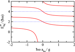
Figure 1. Zero-range energies  as a function of
  . Solid and dotted lines show the energies corresponding to states that are even and odd, respectively, in the relative coordinate.
Download figure:
Standard image High-resolution imageIn addition to using the known properties of  , we take advantage of the fact that the kinetic energy
  of
of  and the
  dependent terms can be combined,

This identity suggests that the momentum-dependent spin–orbit coupling terms add a 'momentum boost' to the solutions  of
of  . Indeed, it is readily verified that the eigenstates of
  ,
,  ,
,  , and
, and  are given by


and

respectively. For fixed g and n and vanishing δ, the states given in equations (6)–(9) are degenerate with eigenenergies  . For
. For  , the degeneracy doubles (see the crossings of the solid and dotted lines in figure 1) since q takes the values
  for
for  that are even in x and the values
  for
for  that are odd in x, i.e., since each of the
  odd in x is degenerate with one of the
  even in x. For non-vanishing δ, the energies are shifted by δ, 0, 0 and
  , respectively. The eigenenergies are simply the sum of a term that depends on the coupling constant g, a center of mass contribution that is characterized by n, a term that depends on the square of the spin–orbit coupling strength
  and a term that depends on the detuning δ.
If Ω is non-zero, the Hamiltonian  expressed in the
  ,
,  ,
,  , and
, and  pseudo-spin basis is no longer diagonal. To determine the eigenenergies and eigenstates for non-zero Ω, we express
  in terms of the eigenstates
  , where σ1 and σ2 take the values
  and
and  . The off-diagonal matrix elements
  ,
,
can be separated into two one-dimensional integrals,

where

and

The sign of the exponent is determined by the pseudo-spin combinations:  ,
,  ,
,  and
and  for
for  ,
,  ,
,  and
and  , respectively.
The integral  over the center of mass coordinate coincides with the Fourier transform of the product of two one-dimensional harmonic oscillator eigenstates. For
 , we find [50]
where  denotes the associated Laguerre polynomial.
The integral  over the relative coordinate can be performed by expanding
 ![${{[{{\phi }_{q^{\prime} }}(x)]}^{*}}$](https://content.cld.iop.org/journals/0953-4075/47/16/161001/revision1/jpb498910ieqn96.gif) and
and  in terms of the non-interacting harmonic oscillator functions
  ,
,  , where the expansion coefficients
  can be obtained analytically [8]. The integral
  then becomes a double sum over integrals that have the same structure as the center of mass integrals
  . In the calculations reported below, we use a finite cutoff
  . The 'optimal' cutoff depends on the value of g considered, the number of relative functions
  included in the basis and the desired accuracy. For
  , we find, as in the g = 0 case, a closed analytical expression for the integral
  . Having analytical expressions for the matrix elements of
  , the eigenenergies can be obtained through matrix diagonalization.
To obtain basis functions with good quantum numbers, we work with linear combinations of the functions given in equations (6)–(9), i.e., we work with the basis functions  and
and  . By properly combining the parts of
  that are even or odd in the relative coordinate and even or odd in the center of mass coordinate, we construct basis functions that are eigenstates of the operators P12 and Y12. The operator P12 exchanges the coordinates (position and spin) of particles 1 and 2. Basis functions that are unchanged under the operation P12 are needed to describe states with bosonic symmetry
  and those that pick up a minus sign under the operation P12 are needed to describe states with fermionic symmetry
  . The operator Y12 can be written as
  , where the parity operator P changes xj
to
, where the parity operator P changes xj
to  (j = 1 and 2). The Y12 operator determines the 'helicity' of the system. We label the eigenstates by
  , where
  and
and  are defined by their actions on an eigenstate. The basis functions with
  symmetry, for example, are given by
  with
with  even and
  even, by
  with
with  even and
  odd, by
  with
with  even and
  even, and by
  with
with  odd and
  even.
even.
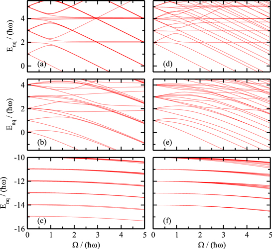
As an example, figures 2(a)–(c) show energy spectra corresponding to eigenstates with  as a function of the Raman coupling strength Ω for vanishing detuning δ, small coupling constant g,
  , and three different spin–orbit coupling strengths
  . The energy spectrum in figure 2(a) is, to leading order, given by the spectrum for
  . In this limiting case, the energies are equal to
  and
and  , where
  . Finite g and
  values introduce shifts and avoided crossings. Specifically, the small positive coupling constant g introduces a positive energy shift for the states that are even in the relative coordinate, which—in first-order perturbation theory—is given by
  . The spin–orbit coupling term introduces, in the small Ω regime, a small down shift that is proportional to
  . This down shift is negligible in figure 2(a) but clearly visible in figures 2(b) and (c). Moreover, the spin–orbit coupling introduces avoided crossings. The broadest avoided crossings occur around
  , where states with the same q but n quantum numbers that differ by one are coupled. The reason is that the spin–orbit coupling term connects, via the total momentum operator, states in first-order perturbation theory if the states' n quantum numbers differ by one and in higher-order perturbation theory otherwise.
Figure 2. Eigenenergies Enq
corresponding to eigenstates with  as a function of
  for
for  , and (a)
  and
and  ; (b)
; (b)  and
and  ; (c)
; (c)  and
and  ; (d)
; (d)  and
and  ; (e)
; (e)  and
and  ; and (f)
  and
and  , respectively.
Download figure:
Standard image High-resolution image
Figures 2(d)–(f) show energy spectra for the strong coupling limit, i.e., for  , as a function of the Raman coupling strength Ω for vanishing detuning δ. To facilitate the comparison between the large and small g limits, the spin–orbit coupling strengths
  in figures 2(d)–(f) are the same as in figures 2(a)–(c). In the regime where
  , the energies change approximately linearly with Ω (with positive, vanishing or negative slope). When
  , the low-lying portion of the energy spectrum consists of approximately parallel energy levels that can be parameterized as
  , where c is a constant.
As already aluded to in the introduction, the theoretical framework developed can be generalized to higher-dimensional trapping geometries. For a spherically symmetric 3D system, e.g., the eigenstates of the 3D Hamiltonian  with 3D contact interaction can be expanded in terms of products of 2D and 1D harmonic oscillator states using cylindrical coordinates. As in the 1D case pursued in this work, the matrix elements for the higher-dimensional system can be calculated analytically. Axisymmetric harmonic traps with spin–orbit coupling in one direction can be treated analogously. Furthermore, using the eigenstates of the trapped three-particle system in 1D, 2D or 3D with contact interactions [11, 22, 23] and expressing the three-particle Hamiltonian in terms of the eight pseudo-spin states, a non-zero Ω introduces off-diagonal elements that can be calculated analytically following steps similar to those discussed in this paper.
Summarizing, this work introduced a theoretical framework that allows for the efficient determination of the energy spectrum and eigenstates of the trapped two-particle system in 1D with contact interaction and spin–orbit and Raman coupling terms. The energy spectra show a rich dependence on the interaction, spin–orbit and Raman coupling strengths. The framework presented provides an important stepping stone for treating more complicated systems with spin–orbit coupling, such as higher-dimensional two-body systems and three-body systems.
Acknowledgements
Support by the National Science Foundation through grant number PHY-1205443 and insightful discussions with P Engels are gratefully acknowledged. DB and XYY acknowledge support from the Institute for Nuclear Theory during the program INT-14–1, 'Universality in Few-Body Systems: Theoretical Challenges and New Directions'.