

Abstract
Attosecond science, born at the beginning of this century with the generation of the first bursts of light with durations shorter than a femtosecond, has opened the way to look at electron dynamics in atoms and molecules at its natural timescale. Thus controlling chemical reactions at the electronic level or obtaining time-resolved images of the electronic motion has become a goal for many physics and chemistry laboratories all over the world. The new experimental capabilities have spurred the development of sophisticated theoretical methods that can accurately predict phenomena occurring in the sub-fs timescale. This review provides an overview of the capabilities of existing theoretical tools to describe electron and nuclear dynamics resulting from the interaction of femto- and attosecond UV/XUV radiation with simple molecular targets. We describe one of these methods in more detail, the time-dependent Feshbach close-coupling (TDFCC) formalism, which has been used successfully over the years to investigate various attosecond phenomena in the hydrogen molecule and can easily be extended to other diatomics. In addition to describing the details of the method and discussing its advantages and limitations, we also provide examples of the new physics that one can learn by applying it to different problems: from the study of the autoionization decay that follows attosecond UV excitation to the imaging of the coupled electron and nuclear dynamics in H2 using different UV-pump/IR-probe and UV-pump/UV-probe schemes.
Export citation and abstract BibTeX RIS
1. Introduction
The 21st century has seen the development of radiation sources capable of emitting light pulses with an attosecond (as) duration [1, 2], opening the way to the observation of electronic motion in atoms and molecules at its natural timescale. The so-called attosecond revolution [3] includes an impressive succession of experimental achievements during the first decade of the century in approaches based on high-order harmonic generation (HHG) from gases. These include the implementation of laser amplifiers for carrier envelope phase stabilization in few-cycle pulses [4], a variety of amplitude and temporal gating techniques [5–8], and different autocorrelation [9] and cross-correlation methods [10, 11] for characterizing the temporal profile of the pulse. The demonstration of the generation of attosecond pulses [1] and the experimental realization of the first train of attosecond pulses [2] came together in 2001. These accomplishments gave birth to the first fully characterized isolated few-cycle pulse in 2006 [12], with a duration of 130 as and a central frequency of  eV. Note that the period associated with 35 eV radiation is 118 as, with this being the lower time limit for a Fourier-limited single cycle pulse of that frequency. The 100 as barrier was soon broken using new techniques employing single cycle near-infrared (NIR) radiation, reaching 80 as with 80 eV pulses [13], or combining gating techniques (double optical gating, DOG) [14, 15] to produce pulses as short as 67 as with central energies of 90 eV [15].
Despite the rapid progress made in these years, this technology is in fact the result of more than five decades of research in three areas that merged together: laser science, collision physics and non-linear optics. The theoretical side of these developments has played more than a mere supporting role. In fact, key techniques for the generation of ultrashort pulses themselves were implemented following solid theoretical predictions, such as the well-known three-step model [16–18] for HHG or the polarization gating method [19]. Moreover, successful experimental applications for attosecond pulses have usually been guided and preceded by numerical simulations. For instance, a large number of theoretical works on electron–electron correlation to control the dynamics in the vicinity of autoionizing states in the helium atom (see references in [20]) were performed before its experimental demonstration [20]. Another example is the first attempted XUV-pump/XUV-probe experiment to explore the coupled electron and nuclear dynamics in the hydrogen molecule [21], which followed the scheme previously proposed in a theoretical work [22]. Theory also had a prominent role in the photoionization of more complex systems, as demonstrated by quantum chemistry simulations performed around ten years ago [23, 24] that predicted the ultrafast timescales for charge migration in biological molecules and whose experimental evidence was achieved only very recently [25, 26]. The predictive potential of any theoretical tool lies on the level of its approximations, which often depends on the size of the target. Current efforts seek to improve the accuracy of theoretical methods and their capability to describe larger systems, but approaches that are able to deal with non-perturbative fast electronic dynamics induced by ultrashort laser pulses in molecular systems remain scarce.
We focus here on methodologies that describe the interaction of molecules with attosecond pulses in the frequency domain of the ultraviolet (UV) and extreme ultraviolet (XUV). This light is currently generated in table-top devices that make use of HHG and in large-scale facilities such as free electron lasers (FELs). Although the typical intensities of the pulses generated by FELs can be very large, their short wavelengths ensure a negligible distortion of the molecular potentials (perturbative regime), thus allowing one to interpret the induced photodynamics in terms of potential energy curves. A few works have already given the first hints on the evolution of electron wave packets created upon photoionization in targets such as large amino acids [26, 27], and even in chains of amino acids [24], which were explored in the first experiments on charge rearrangement and fragmentation [28]. Specifically, these works made use of either density functional theory (DFT) [24, 26] or configuration interaction methods [27] in which the nuclei are kept frozen, which is a reasonable approximation for electronic processes occurring in the sub-fs and few-fs timescale in molecules containing heavy (therefore slow) nuclei. DFT-based methods are commonly implemented using existing software packages [29, 30] and provide energies and electron densities with reasonable accuracy, as long as the single active electron picture remains valid. The configuration interaction methods are capable of describing the correlation between two active electrons, thus opening up the possibility of exploring excitation–ionization processes [27, 31–33]. However, regardless of the methodology chosen, the correct representation of the wave packet created in the electronic continuum in large molecules upon interaction with an attosecond pulse still remains a challenge. Most existing works [24, 27, 31, 33] describe the ionization wave packet as a distribution resulting from a sudden transition from the ground state, e.g, by performing a direct projection of the ground state into the ionic states. A more elaborate approach is used in [26], where the photoionization amplitudes are accurately computed using a combination of a DFT package [30, 34] with a numerical description using B-spline basis sets for the electron in the continuum [26, 35]. This implementation has also been extended to include the nuclear motion within the Born–Oppenheimer (BO) approximation for diatomic molecules [36, 37] or for the symmetric stretching mode in molecules with a small number of atoms [38], although within the framework of time-independent methods.
A promising alternative for exploring electronic dynamics in small molecules is the multi-configurational time-dependent Hartree–Fock (MCTDHF) method [39–43]. A novel implementation of the MCTDHF approach incorporates the nuclear degrees of freedom, even beyond the BO approximation, to treat diatomic molecules [44]. The method has demonstrated a reasonably good agreement with existing accurate photoionization cross-sections for the hydrogen molecule, and the time-dependent implementation to obtain time-resolved images of laser-induced electron dynamics was demonstrated recently [45, 46]. Despite the successful and promising outcomes of these methodologies, a theoretical implementation that treats electronic and nuclear motion on an equal footing beyond the BO approximation is only available for the most simple targets. In this context,  has obviously been the object of a large number of theoretical studies, which have shed some light on the effect of the coupled electronic and nuclear dynamics induced by ultrashort pulses [47, 48]. The next step towards more complex systems, which is the inclusion of electron correlation, remains a challenge. Most theoretical approaches reported to date have explored H2 using the fixed nuclei approximation (FNA) [49–59]. A few works have considered both electronic and nuclear degrees of freedom, while ignoring the dependence of the electronic structure, eigenfunctions and dipole transition moments on the internuclear distance [60, 61]. It should be noted, however, that some of these implementations, even within the FNA, must be considered to be breakthroughs, since they report the first successful attempts to describe one-photon double ionization [53–59] and even two-photon double ionization of H2 [62–64]. In [65], the BO approximation was introduced for the first time to describe double ionization after one-photon absorption. Nevertheless, the two-photon (multiphoton) absorption leading to the four-body Coulomb break-up of the molecule remains unsolved in full dimensionality, i.e., the effect of nuclear motion is still unexplored and the reliability of the existing data within the FNA [62–64] are yet to be probed. None of these methods has been able to represent processes in which electronic and nuclear motion occur in the same timescale, e.g., autoionization, which is the paradigm of electron correlation.
To our knowledge, the only available methodology to describe photoionization problems in H2 (and D2)—including all electronic and nuclear degrees of freedom in the time domain and capable of describing molecular autoionization correctly—is the so-called time-dependent Feshbach close-coupling (TDFCC) method. An early stationary version of this method was introduced in the late 1990s [66, 67], while the first time-dependent implementations were performed in 2006 [68–70]. The latter works and subsequent improvements constitute the main body of this review. The performance of the TDFCC method has been demonstrated by a large number of successful comparisons with experiments in a variety of one- and multi-photon single ionization processes (see, e.g., [71–77]). But its main strength is the possibility it offers to analyze the underlying physics in a simple way, which is crucial to extrapolate to larger molecular systems. Nevertheless, representation of two electrons in the continuum is still a major limitation of this method, although in some specific cases, such as sequential two-photon double ionization, this shortcoming can be successfully circumvented by considering two separate one-photon ionization transitions.
Most applications of the TDFCC method have shown that inclusion of the nuclear degrees of freedom is mandatory to appropriately describe a wide range of laser-induced processes in molecules. For instance, a resonant multi-photon transition may appear as a sharp profile in the photoionization spectrum as a function of photon energy within the FNA, while it is smoothed or even totally washed out when the nuclear motion is included [78]. In particular, to describe autoionization from doubly excited states of H2, the inclusion of nuclear motion is a must, since the timescales for autoionization and dissociation are similar [66, 67, 79]. In this review, the role of nuclear motion and electron correlation in H2 subject to attosecond radiation sources is discussed within the context of the TDFCC method. The versatility of the method is illustrated through a selection of applications in which distinct physical phenomena are induced in the hydrogen molecule when illuminated with single UV attosecond pulses, trains of attosecond UV pulses and pump–probe schemes combining UV with UV or UV with IR pulses.
The paper begins with an overview of the laser parameters that define an attosecond pulse, including a short summary of the time/frequency picture that is at the core of any analysis of dynamical processes in atomic and molecular attoscience. The following section 3, presents a detailed and unified description of the TDFCC method for treating diatomic molecules. We start by explaining the essence of the method [68–70, 72] and go on with a description of earlier molecular electronic structure methods [66, 67, 80], which produce the main ingredients to be used in TDFCC and in any time-dependent implementation based on the spectral approach. Sections 4 and 5 review some interesting applications that use single attosecond or few-fs pulses, and section 6 does the same for those that use combinations of pulses (pump–probe techniques). Finally, in section 7 we summarize the current state, scope and perspectives for this and other theoretical tools in attoscience.
2. Pulsed radiation
The generation of the first attosecond pulse in 2001 [1] came with a renewed interest to understand and manipulate attosecond optics. The advent of new and improved techniques in the generation of ultrashort pulses [81], as well as the development of reliable pulse characterization methods [82], has pushed this field towards the design of novel applications that capture ultrafast processes with an unprecedented time resolution. Using this pulsed radiation to induce and probe electronic and nuclear dynamics in matter first requires a full characterization of the light itself. Accurate retrieval of both the amplitude and phase of the frequency components of isolated or trains of attosecond pulses still poses a challenge for existing experimental techniques [82, 83]. For instance, many table-top HHG techniques produce very short pulses but with a non-stabilized carrier envelope phase, which is a key parameter for many pump–probe and multi-photon studies, as we discuss later. Pulsed radiation is also often produced with background pedestals, leading to a large noise-to-background signal [81] that is difficult to account for in a realistic theoretical description of laser-induced processes. Nevertheless, one can find reasonable approaches to reproduce most experimental conditions and radiation parameters or, at least, those that are relevant to the problem under consideration. Mathematically, an isolated pulse with a duration T can be defined by its vector potential (within the dipole approximation):

where  is the polarization vector and
  =
= ![$F(t)\mathrm{sin}[{\rm{\Phi }}(t)]$](https://content.cld.iop.org/journals/0953-4075/48/24/242001/revision1/jpb518094ieqn5.gif) , with
, with  being the envelope that accounts for the finite duration T and
  the argument in the sine function

where ϕ is the carrier-envelope phase (CEP),  is the carrier-envelope frequency and b is the chirp parameter that introduces a time-dependence of the pulse frequency over time. It is convenient to first define the vector potential,
  , from which the electric field,
  , can be unambiguously derived (
 in SI units). The Fourier transform of expression (1) gives the amplitude and phase of the frequency components of the pulse. Short pulse durations are associated with wide frequency distributions. Consequently, obtaining time images of the ultrafast electronic and nuclear motion with attosecond pulses implies the generation of wave packets that are the result of the coherent superposition of many electronic (vibronic) states of the atom (molecule). As we show below, the use of spectral methods, e.g. TDFCC, has the advantage that one can easily visualize the connection between the pulse frequency spectrum and the distribution of states that constitutes the wave packet resulting from the interaction between the radiation and the atom or the molecule.
The Fourier analysis of different ultrashort pulses using typical values for the parameters defined in equation (2) are shown in figures 1 and 2. The pulses and Fourier transforms are performed using the open source package from [84]. The left panels in both figures show the magnitude of the electromagnetic field  as a function of time, while the right panels display the absolute value and phase of their corresponding Fourier transforms
 ![$\left[\tilde{E}(\omega )={\displaystyle \int }_{-\infty }^{\infty }{e}^{-i\omega t}E(t){\rm{d}}{t}\right]$](https://content.cld.iop.org/journals/0953-4075/48/24/242001/revision1/jpb518094ieqn13.gif) . For all panels in figure 1, we plot a single isolated pulse defined by an electric field as
. For all panels in figure 1, we plot a single isolated pulse defined by an electric field as ![$E(t)={E}_{0}F(t)\mathrm{cos}[{\rm{\Phi }}(t)]$](https://content.cld.iop.org/journals/0953-4075/48/24/242001/revision1/jpb518094ieqn14.gif) with a standard Gaussian profile
with a standard Gaussian profile  =
=  centered at time zero, where the full width at half maximum (FWHM) is
  as in intensity. We modify the CEP and the chirp while all other parameters are kept within typical values for studies of electron dynamics in molecules: a carrier frequency in the UV/XUV region to induce electronic transitions,
  = 30 eV; a pulse length in the fs/sub-fs timescale; and laser intensities that ensure photo-induced processes within the perturbative regime, I=1012 W cm−2. The intensity is related to the field amplitude through the atomic unit of intensity, E0 =
  , with I0 =
  W cm−2. We initially compare two pulses with no chirp (
 )and different CEP (
 in panel (a) and
  in panel (b)). As the Gaussian envelope is centered at zero, the maximum amplitude is thus found at the center of the pulse for CEP
  (panel (a)), while the maximum is shifted by
  for CEP
  (panel (b)). Their Fourier transform leads to identical frequency distributions. This implies that for one-photon absorption processes, one would generate identical wave packets (i.e. containing exactly the same states) except for a global phase
  . It is a frequency-independent phase that will not be observed in a first-order process [85, 86] and it can only be retrieved by studying high-order processes (i.e., multi-photon absorption) or combining such a pulse with a second reference pulse. For isolated pulses, the choice of CEP is only relevant for few-cycle pulses or pulses with asymmetric
  envelopes, since in this case the CEP determines the maximum amplitude reached within the envelope.
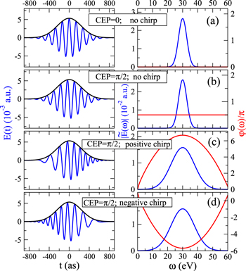
Figure 1. Electric field  in the time domain (left) and
  in the frequency domain (right); the latter is the corresponding complex Fourier transform of the electric field with its absolute value
  in blue and its phase argument
  in red. All pulses are obtained with a Gaussian-shaped envelope for the intensity with 400 as of FWHM in time, a central carrier frequency
  = 30 eV and intensity I = 1012 W
  (see a detailed description of laser parameters in the text). The chirp is defined with respect to the carrier frequency such that b =
  , where γ is given in units of fs−1 and b takes units of fs−2. We choose γ = ±0.5 fs−1 to obtain appreciable chirped pulses with such short durations. (a) CEP ϕ = 0 and chirp parameter b = 0; (b) CEP
  and chirp b = 0; (c) CEP ϕ=
 and positive chirp b = +
 fs−1); and (d) CEP ϕ =
  and negative chirp b = −
 fs−1).
Download figure:
Standard image High-resolution imageIntroducing a chirp, however, has a significant effect in the Fourier transform of an isolated pulse. Panels (c) and (d) in figure 1 show pulses with the same CEP as in panel (b) ( ), but with a different chirp parameter b. The chirp is defined with respect to the carrier frequency such that b =
  , where γ is given in units of fs−1 and b takes units of fs−2. For 1 fs pulses centered at 30 eV we have chosen a rather large chirp, γ = ±0.5 fs−1, so that it can be visualized easily. The case of positive chirp is given in panel (c) and negative chirp is given in panel (d). As can be seen, on the one hand, the introduction of a chirp broadens the frequency distribution. Consequently, by chirping the pulse one can generate a wider superposition of states (or broader wave packet), with an effect equivalent to reducing the pulse duration while keeping the laser-molecule interaction time constant. On the other hand, the chirp incorporates a frequency-dependent phase,
  =
= ![${\mathrm{tan}}^{-1}\frac{{Im}[\tilde{E}(\omega )]}{{Re}[\tilde{E}(\omega )]}$](https://content.cld.iop.org/journals/0953-4075/48/24/242001/revision1/jpb518094ieqn44.gif) , as illustrated by the red lines in the right-hand-side panels of figure 1. In the present example, with a linearly time dependent chirp, we find a maximum (minimum) value for the phase
, as illustrated by the red lines in the right-hand-side panels of figure 1. In the present example, with a linearly time dependent chirp, we find a maximum (minimum) value for the phase  at the central frequency for a positive (negative) chirp parameter. The resulting effect is to imprint a different phase
  to each energy component of the photo-excited wave packet, which may imply a strong modification (useful for control) of the molecular photo-dynamics due to the different nature of the interferences. Phase-shaped femtosecond laser pulses are already being used as a bond-selective technology in chemistry [87, 88]. Currently, significant efforts are being made to tailor optics with the ability to generate sub-femtosecond chirped pulses, with the promise of achieving a similar control of electron dynamics in atoms [89], molecules [90–92] and surfaces [93]. In this review, we only discuss simulations using unchirped pulses, since they are used most frequently in current attosecond science applications. It should be mentioned, however, that synthesizing completely unchirped (Fourier-transformed limited) pulses in a laboratory is also a challenging task due to the intrinsic chirp that is often associated with broadband pulses [82].
The choice of the envelope profile,  , for the laser pulse may also affect the result of the simulations. The most common choices are a Gaussian or a sine/cosine squared function, which provide a smooth switch on–switch off for the field. In the simulations discussed in this review, we use a sine/cosine squared envelope to simplify the numerics, because in contrast to the Gaussian envelope, the time propagation can be turned on/off with the field being exactly zero. Trapezoidal envelopes have also been used, but only for testing purposes. Figure 2 shows a few examples of pulses with different envelopes, namely Gaussian (a), cosine-squared (b) and trapezoidal (c) envelopes, while keeping all the other parameters as in figure 1. Their corresponding Fourier transforms are shown in the right-hand-side panels. For the same FWHM duration in intensity, one obtains slightly different frequency distributions. The frequency spectrum
  of the Gaussian-shaped pulse is the only one that tends monotonically to zero when
  . The frequency distributions of the cosine squared and the trapezoidal envelopes exhibit small side components around the central peak. These components arise from Fourier transforming a finite, non periodic signal. For the same reason, there is an arbitrariness in the phase argument
  , jumping by
  at every frequency at which
  = 0. Note, however, that the existence of these side peaks is not necessarily unrealistic or unphysical, since laboratory pulses are also finite.

Figure 2. Same as in figure 1, but now all pulses are unchirped and have a common CEP  , and different envelopes
  are employed: (a) Gaussian envelope for the intensity with a FWHM of 400 as; (b)
  envelope for the field with a FWHM with an intensity of 400 as; and (c) trapezoidal envelope with T = 1 fs duration with a 300 as ramp.
Download figure:
Standard image High-resolution imageThe advantage of using any of these envelopes is the possibility of extracting their Fourier transforms analytically, which simplifies the calculations and the subsequent analysis. As an example, using equation (1) for the vector potential of the field with a temporal envelope  , one obtains
This specific expression has been used in several theoretical works in the framework of first-order time-dependent perturbation theory for atomic and molecular photoionization [86, 94, 95] and we employ it for the one-photon problems discussed in the next section.
A time shift ( ) of the laser pulse results in the addition of a linearly dependent phase (
 ) in the frequency domain. As for the CEP, it will only be relevant in multi-photon processes or when a reference pulse is present, e.g., in experiments combining two or more ultrashort pulses. This is the case in most existing pump–probe schemes involving ultrashort pulses, which aim to obtain real-time images of electron dynamics. Many of these pump–probe experiments involve IR pulses containing a small number of cycles, so that CEP stabilization is mandatory and even becomes a tuning parameter [96]. In pump–probe schemes that only make use of pulses that contain a large number of cycles, an accurate evaluation of the relative phases between the pulses may also be needed. For example, an approach that has been used recently because of its relatively easy experimental implementation uses two identical but delayed pulses [21, 74, 75], so that the same source generates the pump and the probe. The experimental challenge in this case is the CEP stabilization in order to generate exact replicas of a given pulse. Mathematically, the vector potential describing a pump–probe scheme using twin pulses can be written as
  , where
  is deduced from equation (1) and the field is obtained through
  and τ is the time delay between the pulses, i.e. the elapsed time between the center of each pulse. The Fourier transform is linear and consequently additivity applies, so that the Fourier transform of the composed pulse now reads

whose squared absolute value leads to a cosine-modulated signal

A zero time delay, τ = 0, implies the sum of two identical pulses, equivalent to a single pulse with twice the amplitude, i.e., it is four times more intense. In figure 3, the electric field  for twin 2-fs pulses with different time delays between them is plotted and the corresponding Fourier transforms are given in figure 4. As explained above, we first define the vector potential with a
  temporal envelope and then derive the field
  that is plotted. In this specific example, we used an intensity of I = 1012 W cm−2 and a central frequency
  = 12 eV. An ideal pump–probe scheme would imply that the probe pulse arrives after the pump pulse, in other words, that
  for identical pulses or
  for a general pump–probe scheme with pulses of different durations T1 and T2. However, most experimental setups include measurements for small time delays, where both pulses overlap. This case is shown in the left panels of figures 3 and 4. For these overlapping pulses, we find that destructive (constructive) interferences change the frequency distribution significantly. In fact, the sum of the overlapping pulses leads to electric field envelopes that are similar to those of a single pulse but with longer duration and lower intensity. Consequently, one should expect narrower frequency distributions in figure 4. For instance, in figure 3, for a time delay τ = 1 fs, the total field looks like a trapezoidal finite pulse whose frequency distribution (see figure 4) is similar to that of a trapezoidal pulse (see figure 2).

Figure 3. Electric field  resulting from the addition of two identical laser pulses with electric fields
  and
and  for different time delays τ. Pulse parameters: T = 2 fs,
  = 12 eV and I = 1012 W
  . For reference we plot the field of the single pulse in all panels (thin gray line).
Download figure:
Standard image High-resolution image
Figure 4. Absolute value of the Fourier transform  of the electric fields corresponding to the sum of two identical pulses separated by different time delays τ, as plotted in figure 3. For reference we now plot the Fourier transform for two identical pulses with zero delay, i.e. 2
 $](https://content.cld.iop.org/journals/0953-4075/48/24/242001/revision1/jpb518094ieqn74.gif) (thin gray line).
(thin gray line).
Download figure:
Standard image High-resolution imageAs long as the pulses do not overlap (time delays longer than 2 fs in our specific example), the Fourier transform gives a peaked pattern in the frequency domain, matching the ![$[1+\mathrm{cos}(\omega \tau )]$](https://content.cld.iop.org/journals/0953-4075/48/24/242001/revision1/jpb518094ieqn75.gif) -modulated analytical expression. Using, e.g., the first order time-dependent perturbation theory formalism, one can easily understand that the structure of the Fourier transform of the pulse should reflect in the excitation/ionization probabilities as a function of energy. To illustrate this point, we show in figure 5 the excitation probabilities (accurately calculated with the TDFCC methodology) as a function of final vibronic energy for a hydrogen molecule initially in its ground state
-modulated analytical expression. Using, e.g., the first order time-dependent perturbation theory formalism, one can easily understand that the structure of the Fourier transform of the pulse should reflect in the excitation/ionization probabilities as a function of energy. To illustrate this point, we show in figure 5 the excitation probabilities (accurately calculated with the TDFCC methodology) as a function of final vibronic energy for a hydrogen molecule initially in its ground state  (vg = 0), which is irradiated by the twin pulses shown in figure 3. Figure 5 shows the vibrational populations in the first electronic excited state B
  of the hydrogen molecule resulting from the interaction with the twin pulses. One can see that at each time delay the resulting vibrational distribution reflects the frequency spectrum given in figure 4. These vibrational distributions are additionally modulated by the electronic dipole transition moment and the Frank–Condon distribution, which is very similar to the vibrational distribution obtained at zero time delay (shown in gray). In order to obtain such well-defined interference patterns in a real experiment it is essential that the pump and probe pulses are exact replicas, which implies a steady CEP, negligible or removable pedestals and zero chirp. Obviously, in these pump–probe schemes, the interesting physics arises when the relative phases among those states (the stationary phases plus the phase imprinted by the pulse at each frequency) is retrievable. This requires that higher order processes come into play, e.g., two-photon absorption distributions, which will map the dynamics launched in those excitation channels.

Figure 5. Excitation probabilities to the bound states of the B  state of H2 upon one-photon absorption after the interaction of two identical ultrashort pulses (
 = 12 eV, T = 2 fs and I = 1012 W
  ). The x-axis stands for the vibronic energy referred to the ground state
  (
( ) (see figure 6). The time delay between the pulses is indicated in each panel. For comparison, the result for zero delay is plotted in all panels as the gray background distribution. As discussed in the text, the distributions closely follow the peaked patterns given by the absolute squared value of the Fourier transform of the field given in figure 4.
Download figure:
Standard image High-resolution imageIn the following section, we describe the TDFCC spectral method and illustrate its suitability to easily disentangle the dynamical information from other features, which are nothing but simple spectral effects from the use of broadband pulses.
3. Theory
In 1999, Journal of Physics B published a topical review by one of the authors [97] that described the ionization and dissociation of the hydrogen molecule by one-photon absorption from cw radiation. The review described the theoretical developments to deal with the electronic and nuclear continuum of H2 using  integrable functions based on B-splines expansions. In particular, it presented the first fully correlated description of the resonant continuum wave function for the molecular doubly excited states, providing a practical method to evaluate accurate widths and energy positions of these autoionizing states and disclosing their role in the dissociative and non-dissociative photoionization of H2. The weak light–molecule interaction was described using a stationary approach based on first order perturbation theory, thus limiting the applicability of the method to one-color, one-photon absorption processes [66, 67, 80]. In this paper, we review the progress achieved since then in treating time-dependent problems beyond the perturbative case, which led in 2006 [68, 72] to the first time-dependent theoretical description of the combined electron and nuclear dynamics in resonant dissociative photoionization of H2 induced by ultrashort laser pulses. This dynamical picture has become mandatory in the last few years to guide and interpret state-of-the-art experiments on H2 molecules irradiated with pulses of different colors or with sub-fs ultraviolet pulses.
The presentation of the theory is organized in seven subsections, starting in section 3.1 with a formal and general description of an implementation of the Feshbach formalism [98] for the solution of the time-dependent Schrödinger equation (TDSE) in the context of molecular photoionization. This implementation is henceforth called the time-dependent Feshbach close coupling (TDFCC) method. In the following four subsections, from 3.2 to 3.5, we describe how to construct the molecular vibronic states, especially those associated with ionization and dissociation channels. We first introduce in section 3.2 some general remarks on the use of B-spline basis sets that are employed to describe both electronic molecular orbitals and nuclear wave functions. This is then followed by two sections dedicated to the computation of electronic states: section 3.3 focuses on the electronic continuum and section 3.4 on the bound and resonant states embedded in the electronic continuum. The methodology to calculate the unperturbed molecular states closes in section 3.5 with the inclusion of the nuclear degrees of freedom. A short account of some specific technical issues in the numerical implementation of the method is given in section 3.6. We conclude in section 3.7 with the expressions that connect the time-dependent amplitudes resulting from the solution of the TDSE to the total, angle- and energy-differential observables. Although the TDFCC formalism presented in section 3.1 is applicable to any diatomic molecule (and to polyatomic molecules if conveniently generalized to include more than one nuclear degree of freedom), for the sake of simplicity, in the following sections it is applied to the H2 molecule, for which the method has been thoroughly used. In this theory section, expressions are given in atomic units except in section 3.7 to retain the dimensional analysis.
3.1. Time-dependent feshbach close-coupling method
The total non-relativistic Hamiltonian for the internal motion of a diatomic molecule with two nuclei A and B, with masses MA and MB and nuclear charges ZA and ZB, and n electrons whose coordinates are referred to the geometrical center of the nuclei, can be expressed as
where MT = MA+MB is the total nuclear mass, μ =  is the reduced nuclear mass and R =
  =
=  is the internuclear distance. For a homonuclear molecule, e.g., H2, MA = MB, the last term in equation (6) is strictly zero. As
  , the mass polarization terms
  and the
  terms can be neglected. Furthermore, we can now fix the molecular axis to reduce the size of the problem by removing the two Euler angles that describe the orientation of that axis in space. By further removing the three coordinates associated to the total centre of mass, the description of the quantum system remains with
  coordinates, that is the internuclear distance R plus the
  coordinates of the n electrons (denoted
  for short). Henceforth we will deal with the following approximate Hamiltonian

where  =
=  is the relative kinetic energy of the nuclei and
 ![${\hat{{\mathcal{H}}}}_{{el}}={\sum }_{i=1}^{n} [-{{\rm{\nabla }}}_{i}^{2}/2-{Z}_{A}/ | {{\bf{r}}}_{i}-{{\bf{R}}}_{A}| -{Z}_{B}/| {{\bf{r}}}_{i}-{{\bf{R}}}_{B}| ]\;+ ({Z}_{A}{Z}_{B})/R$](https://content.cld.iop.org/journals/0953-4075/48/24/242001/revision1/jpb518094ieqn96.gif) is the electronic Hamiltonian with a parametric dependence on the nuclear coordinate R.
is the electronic Hamiltonian with a parametric dependence on the nuclear coordinate R.
The rotational degrees of freedom can be simply neglected when considering the timescales of interest in the sub-fs regime. Indeed, the rotational motion occurs in the picosecond regime, thus it is approximately three orders of magnitude slower than vibrations (typically taking place in tens of fs) and five to six orders of magnitude slower than electrons (attosecond regime). More importantly, the availability of kinematically complete experiments [99] along with ultrashort laser pulses of attosecond duration [6] has opened the way to work with fixed-in-space molecules. Indeed, in these experiments, the axial recoil approximation [100] is used to analyze the results since, after photo-absorption in the continuum, the time employed by the molecule to dissociate is much shorter than the rotational period of the molecule. In practice, it means that in dissociative ionization processes the set of vectors ( ,
,  ,
,  ), where
  is the momentum of the A+ ion,
  is the electron momentum and
  is the polarization direction, are measured in coincidence and can therefore be assigned to the body-fixed-frame triplet of vectors (
 ,
,  ,
,  ) for a given nuclear orientation of the molecular axis
  . To fully solve a quantum system with
  independent coordinates is still a very demanding task, even for the seven-dimensional H2 problem
  .
.
The wave function that describes the state of a molecule when interacting with a laser pulse is given by the solution of the TDSE:

where  is the total Hamiltonian,
  =
=  +
+ . Here
  represents the unperturbed Hamiltonian of the molecule described by equation (7), and
  is the time-dependent laser–molecule interaction potential. The TDSE must be solved by assuming that the molecular wave function is known at time t = t0, i.e., before the laser–molecule interaction takes place. In this paper, the TDSE will be solved using the spectral method, in which the wave function
  is expanded in the basis of eigenstates resulting from the diagonalization of the unperturbed Hamiltonian
  (the so-called close-coupling expansion). This approach has been widely used in atoms [101, 102] to describe ionization processes, even in the presence of autoionizing states. Usually, the integral over eigenstates representing the ionization continuum is replaced by a sum over discretized continuum states that result from the diagonalization of
  in a box. In general, the box must be large enough to provide a dense enough spectrum in the continuum that allows one to unambiguously resolve resonant states. In molecules, the practical implementation of this idea is not straightforward due to the presence of the nuclear degrees of freedom. Indeed, in general, electronic and nuclear degrees of freedom cannot be separated, unless in the framework of the BO approximation. However, this is not a good approximation when resonances are present, since the autoionization lifetime of these resonances can be comparable to the time needed by the nuclei to move. Thus, the general assumption behind the BO approximation, which is that electrons are much faster than nuclei, no longer holds in this context. Therefore, in order to obtain a meaningful basis of molecular eigenstates, one should diagonalize the whole molecular Hamiltonian
  , not only the electronic Hamiltonian
  . As a consequence, in the molecular case one must expand the time-dependent molecular wave function in a basis of vibronic states, in which electronic resonances are somewhat diluted and difficult to identify. Another difficulty arises when the autoionization decay time is very long, since in this case dissociation may occur well before the electron is ejected. In other words, a state that could potentially autoionize might not do it and behave as a truly bound state that dissociates into neutral species. This dual behavior of resonances does not exist in atoms because there are no sufficiently fast competing processes that can suppress autoionization.
To avoid diagonalizing the total molecular Hamiltonian  , we will adapt the stationary Feshbach theory for the solution of the TDSE. The original Feshbach projection method [98] was introduced in atoms by O'Malley et al (see [103] and references therein) and its extension to molecular systems was developed later [66, 67], following the seminal works of Bardsley [104] and Hazi, and Rescigno and Kurilla [105]. The Feshbach formalism is based on the introduction of projection operators
  and
and  , satisfying completeness (
 +
+ = 1), idempotency (
 =
=  ,
,  =
=  ) and orthogonality (
 =
=  = 0), which project the total molecular wave function onto non-resonant scattering-like and bound-like states, respectively. By using these projection operators, the molecular time-dependent wave function
 (in the combined space of electronic and nuclear coordinates) can be split off and represented by the state

By inserting the latter equation in the TDSE (equation (8)) and projecting separately in both orthogonal subspaces, one obtains two time-dependent coupled equations, that in matrix form read
One of the advantages of writing the TDSE in this way is that non-adiabatic effects are expected to be small within the resonant  and non-resonant
  subspaces. If one neglects non-adiabatic effects, the nuclear kinetic energy and the projection operators commute such that
 ![$[{\hat{T}}_{N}(R),{\mathcal{Q}}]$](https://content.cld.iop.org/journals/0953-4075/48/24/242001/revision1/jpb518094ieqn134.gif) =
= ![$[{\hat{T}}_{N}(R),{\mathcal{P}}]$](https://content.cld.iop.org/journals/0953-4075/48/24/242001/revision1/jpb518094ieqn135.gif) = 0 and
= 0 and  =
=  = 0. This means that the resonance–continuum coupling is entirely due to the electron–electron interaction, i.e., to
  (or its Hermitian conjugate
  ). This is usually a very good approximation since autoionization lifetimes of doubly excited states are almost exclusively due to the electron–electron interaction. Using these commutation rules, the total molecular Hamiltonian can be further separated in a block-diagonal unperturbed Hamiltonian [
 =
=  ⊕
⊕  ] plus a total interaction potential [
 =
=  +
+ +
+ ], which contains the explicit time-dependent term due to the laser–molecule interaction and two time-independent coupling terms that account for autoionization:
We use a spectral method to solve this coupled TDSE by expanding the total time-dependent wave function in terms of the eigenstates of the unperturbed Feshbach Hamiltonian  =
=  ⊕
⊕ , from which we can build up a complete basis of vibronic states. Following common usage in theoretical chemistry, each vibronic state is written as a product of an electronic wave function
  describing the nth electronic state and a one-dimensional vibrational function
  , where vn is the vibrational quantum number associated to the nth potential energy curve. We note that, for dissociative states, vn is a continuous index. Methods to obtain the vibrational wave functions are discussed in detail in section 3.5. The complete set of vibronic states includes (i) the BO wave functions
  with total energies
  , which are approximate solutions of the
  eigensystem (α denotes a given ionic threshold,
  is the electron kinetic energy in excess above the ionic threshold α,
  is its angular momentum and
  is the vibrational energy of state
  in the potential energy curve of the electronic state α); (ii) the BO wave functions
  with total energies
  , which are approximate solutions of the
  eigensystem; and (iii) the vibronic states associated to the electronic bound states
  with total energies
  . These bound states mostly pertain to the
  subspace. However, in practice, they are more conveniently computed without the Feshbach partitioning.
The expansion of the total time-dependent wave function in our basis of BO vibronic states is written in the Schrödinger picture as:
To solve the TDSE defined in equation (8), we introduce the latter ansatz in equation (11) to obtain a system of coupled linear differential equations that can be written in compact matrix-vector form as (in the interaction picture)
The couplings due to the time-dependent laser interaction,  , correspond to the dipole matrix elements in the long-wave approximation (
 in length gauge and
  in velocity gauge) times the dependence on the laser pulse, i.e.
  =
=  in the length gauge and
  =
=  in the velocity gauge. The crossed terms
  +
+ are active during and after the interaction with the laser pulse. For atoms, this term becomes zero when the resonance (doubly excited) states are fully depleted, so that
  = 0 and
  =
=  (for an application of the present TDFCC method to atoms see [106]). However, this is no longer true for molecules, because the time needed to dissociate into neutrals may be shorter than the autoionization lifetimes, and as a consequence part of the wave function norm can remain in the
  subspace. In other words,
  =
=  , where
  is the asymptotic representation of the dissociative channels in which no ionization has occurred. As in atomic systems,
  =
=  , where
  is the asymptotic representation of the ionization channels. Asymptotically,

so that, in that limit, the eigenfunctions of  and
and  are also eigenfunctions of the total Hamiltonian. Therefore, the expansion coefficients
  of the
  subspace truly represent physical ionization amplitudes once the system reaches its stationary asymptotic limit. The most attractive feature of the present time-dependent Feshbach formulation is that it provides a straightforward interpretation of autoionization processes in time, in contrast to the Feshbach stationary approach [80]. In the time-dependent formulation, the total scattering wave function is built up during time propagation, which allows for the simultaneous excitation of the resonant
  and non-resonant
  subspaces from the initial ground state and their mixing through the interaction potential
  . Again, since we are using a representation of the time-dependent wave function in a basis of molecular states, the transition amplitudes are directly related to the expansion coefficients in equation (12) at
  .
.
The present spectral method has an added advantage regarding computational effort, since the calculation of dipole and  coupling matrix elements included in the interaction potential terms
  in equation (13) is only performed once. The specific laser parameters entering in
  appear as trivial factors, so that in practice one must only invest computer effort in solving the system of coupled linear differential equations (13) for each specific laser field. This is very convenient, because the calculation of the coupling matrix elements is by far the most demanding part from the computational point of view. Indeed, the evaluation of these couplings involves electronic and vibrational states and integrals between them, accounting for both the
  and R dependences. For instance, the matrix elements in the last column of the matrix representation of the TDSE in equation (13) represent the coupling between final vibronic states,
  and (i) initial or intermediate vibronic bound states
  (upper block), (ii) intermediate vibronic resonant states
  (middle block) and (iii) intermediate electronic continuum states
  that account for above threshold ionization processes (lower block). These couplings have the general form

where n represents the labels required for the states in any of the above-mentioned cases and ![$[0,{R}_{\mathrm{max}}]$](https://content.cld.iop.org/journals/0953-4075/48/24/242001/revision1/jpb518094ieqn200.gif) indicates the extension of the nuclear radial box. To compute these vibronic couplings, it is then required to calculate first the electronic matrix elements
indicates the extension of the nuclear radial box. To compute these vibronic couplings, it is then required to calculate first the electronic matrix elements  in a dense grid of internuclear distances within the interval
 ![$[0,{R}_{\mathrm{max}}]$](https://content.cld.iop.org/journals/0953-4075/48/24/242001/revision1/jpb518094ieqn202.gif) , namely, the dipolar transition matrix elements
, namely, the dipolar transition matrix elements  with
with  =
=  (length) or
  =
=  (velocity) as well as the electrostatic Feshbach couplings
  responsible for the resonance decay into the continuum. Consequently, suitable electronic and nuclear structure calculations are needed to generate the set of vibronic states and their energies
  . The calculation of vibronic states for electronic bound states is rather standard, while it is not so trivial for continuum states, especially when both the electronic and the nuclear continuum are involved.
In the following, we describe the method that we have used to obtain the vibronic states used in the close-coupling expansion of the time-dependent wave function. Readers not interested in these technical details may skip this section and go directly to section 4, where a number of different applications of the TDFCC method are discussed.
3.2. One-electron diatomic molecule orbitals using B-splines
For the computation of n-electron (bound, resonant and continuum) molecular states of a diatomic molecule, one can make use of a configuration interaction (CI) method based on expansions in terms of antisymmetrized products of one-particle wave functions. For this, the molecular orbitals for the one-electron molecular ion ( ) must firstly be computed. Consistently with equation (6), they are eigensolutions of the Schrödinger equation
This molecular two-center Coulomb system is a well known exactly solvable problem in molecular physics. It represents, e.g., the  molecule (ZA = ZB = 1). The Schrödinger equation (16) is fully separable in prolate spheroidal coordinates (see for instance [107]) and both energies and wave functions can be computed with arbitrary precision [108–110]. This one-electron molecular Hamiltonian, which we call
  , remains invariant under the rotation of the internuclear axis for both heteronuclear (point group
  ) and homonuclear molecules (point group
  ) and, consequently, it commutes with the operator
  such that the molecular orbitals can simultaneously be eigenstates of
  and
and  . The value of the quantum number λ =
  corresponds to the absolute value of the eigenvalue of the angular momentum operator
  along the internuclear axis Z.
The use of the exact one-electron diatomic molecular (OEDM) orbitals in an n-electron configuration interaction approach along with a scheme well suited to describe the electronic continuum is rather cumbersome [97]. To avoid the difficulties inherent to using non- states and to recover the essence of the partial wave analysis common to many scattering problems, the one-electron wave functions can be expressed in terms of a one-center spherical expansion. For a fixed value of m, the expansion reads

where  refers to the spherical harmonics and we have kept the value of m with its sign to make clear that different values of m must be combined with their respective signs when preparing n-electron configurations. The radial wave function
  can be expanded in terms of suitable basis functions for each internuclear distance R. Our choice for the basis set is B-splines and, therefore,
  =
=  , where NB is the number of B-spline functions. B-splines are piecewise polynomials of order k defined inside a radial box of length
  [111]. The set of k B-splines at the electron position r is constructed by defining a knot sequence
  within the electronic radial box with
 ![$r\in [0,{r}_{\mathrm{max}}]$](https://content.cld.iop.org/journals/0953-4075/48/24/242001/revision1/jpb518094ieqn227.gif) , using the recursion formula [111, 112]
, using the recursion formula [111, 112]

and setting the B-splines of order k = 1 as  for
for  , and
, and  otherwise. The two-boundary eigenvalue problem is solved subject to the boundary conditions
  =
=  = 0, which are automatically satisfied by removing the first
  and the last
  B-spline from the original set.
The latter expansion turns the solution of the original set of differential equations into a generalized eigenvalue problem  = 0 for each internuclear distance R, where
  is the vector for the expansion coefficients
  . The matrix elements of the Hamiltonian and the overlap in terms of the basis
  , for fixed m and R, are

respectively. The size of the one-electron eigensystem is  .
.
In contrast to atoms, the use of a one-center wave function expansion to describe a molecular two-center problem imposes that the electron-nucleus Coulomb potential  is more conveniently expanded in spherical coordinates. When the origin of the one center expansion coincides with the nuclear center of mass, the resulting effective Hamiltonian expressed in spherical polar coordinates is
where  = min(
 ),
),  = max(
 ) and
) and  are the spherical angles of nucleus q=
 . Accordingly, the corresponding matrix elements for the one-electron Hamiltonian adopt the form

where the kinetic energy term
is block diagonal in  and the matrix elements for the Coulomb interaction read
In the latter expressions all angular integrals are analytical (Gaunt formula) and the radial ones can be readily computed to machine accuracy using a Gauss–Legendre quadrature since the integrands are reduced to polynomials (except the Coulomb potential terms). Incidentally, since we adopt a geometry where the linear molecule is oriented along the Z-axis and the origin is located at the nuclear geometrical center in homonuclear molecules, the spherical harmonics for the nuclei  adopt simple constant values for
  =
=  and
and  =
=  , namely,
  =
= 

 =
= if mq=0 and they are identically zero if
  . Given that the pair
  satisfies
  and
and  = 0 (with the only contribution from mq = 0 and m = −m') the quality in the representation of the molecular Coulomb interaction depends on the number of angular momenta
  introduced in expansion (17). Notably, this number must increase as the internuclear distance increases since departure from the atom-like spherical symmetry becomes more pronounced.
In the case of homonuclear molecules, ZA = ZB, the electronic wave function has an inversion symmetry, ![$\hat{i}[\varphi ({\bf{r}})]$](https://content.cld.iop.org/journals/0953-4075/48/24/242001/revision1/jpb518094ieqn263.gif) =
=  =
=  , and it remains unchanged (π = +1 or gerade (g)) or it changes its sign (π = −1 or ungerade (u)) against inversion of the electronic coordinates. In our single center expansion, the inversion symmetry operation only affects the spherical harmonics, i.e.,
  =
=  and, consequently, only even values of the angular momentum contribute to orbitals of gerade symmetry and odd values to orbitals of ungerade symmetry. Furthermore, because both the angular momentum operator
  and the inversion parity operator
  commute with the electronic Hamiltonian
  , separate calculations can be performed for the different values of λ = 0 (σ), λ = 1 (π), λ = 2 (δ), λ = 3 (ϕ), etc, and for gerade and ungerade symmetries, using angular momentum expansions with
  . Typically, for the computation of
  orbitals, one can use a set of 180 B-splines of order k=8 in a linear sequence of knot-points enclosed in an electronic radial box of length
  =60 a.u. with an expansion using only even partial waves in equation (17) from
  =0 up to
  = 16. Note that different angular momenta will contribute for each symmetry. To compute
  orbitals (
 ) the partial waves included are
  , while for
  molecular orbitals (λ = 2) the wave function is expanded in terms of seven odd partial waves with
  = 3, 5, ..., 15.
It is worth noting that, in spite of the advantages of using B-splines in the representation of the continuum [112], there are a few limitations on the reliability of the subsquent CI procedure. In fact, these orbitals fail to accurately reproduce the inner electronic density close to the nuclei around the equilibrium distance. To improve the description of bound states in the case of H2, the CI representation of the inner wave function is usually complemented with additional Slater-type orbitals (STOs), i.e., functions of the type  (typically using n = 1–10,
  0–11 and
  = 2.8 for all n and
  ). For convenience, these supplementary STO basis functions are expanded in the same basis of B-splines. Despite the loss of strict orthogonality and the inclusion of the corresponding overlaps, this addition significantly improves the energy convergence for the ground state in H2 close to the internuclear equilibrium distance Re ∼1.4 a.u.
In principle, with the solution of the one-particle Hamiltonian we have at our disposal a full set of approximate OEDM orbitals  and also their corresponding electronic energies
  . In the case of H2, the latter energies represent the ionization energies at different values of R. A clear disadvantage of one-center expansions is their slower convergence as one moves away from the spherical symmetry at R = 0; the eigenvalues can reproduce the exact OEDM energies [109] at large internuclear distances only at the cost of huge angular momentum expansions, which become impractical. This issue can still be circumvented. First, in most applications, e.g. in H2, the molecule is initially in its ground state, with a density localized close to the equilibrium internuclear distance, and the computed dipole matrix elements can easily be converged up to a rather large value of R. Secondly, although the slow convergence at large internuclear distances may affect the R-asymptotic behavior and the energies of the vibronic wave functions, and by extension the continuum (dissociating) nuclear wave functions, the problem can be overcome by using accurate potential energy curves resulting from standard quantum chemistry calculations for the ground and singly excited states (see, e.g., [113] for the H2 molecule) and/or the exact OEDM potential energy curves for the ionic thresholds.
3.3. Electronic continuum states in  space
space

The molecular non-resonant electronic continua are the eigenstates of the  projected electronic Hamiltonian. One has to solve the eigenvalue problem

for each internuclear distance R. Henceforth we will use a more compact notation and define a collective channel index, μ = (α,  ), encompassing the previously defined ionic threshold label α, with energy
  , and the angular momentum of the scattered electron
  (
( from now on) that is compatible with the molecular symmetries of the
  -electron target. Also,
  .
.
The total electronic energy of the n-electron system satisfies E =  +
+ , where
  is the potential energy curve of the ionic threshold α (in the case of H2, it is simply one of the OEDM energies from the set
  previously described) and
  is the kinetic energy for the emitted electron in channel μ. In our implementation, instead of explicitly calculating the eigenstates of the projected Hamiltonian in equation (25), we use multichannel scattering theory to evaluate electronic continuum states from a basis that spans the
  subspace. Thus we solve instead

where  is the incoming scattering wave function that represents one electron being ionized from the molecule. It is constructed to be an eigenfunction of the set of operators
  (plus
(plus  in the case of a homonuclear molecule) with their corresponding eigenvalues
  (and π). S is the total electronic spin, Ms is its z-component, Λ the absolute value of the z-component of the total electronic angular momentum (
 ), σ is the reflexion symmetry with respect to the XZ plane (±1) and π is the symmetry with respect to the inversion center (g for gerade and u for ungerade).
This projected wave function, for the channel μ and total electronic energy E, is built through a multichannel close-coupling expansion in the form (for notational simplicity, in the rest of the formulation we will consider the case of a two-electron molecule, so that spin functions can be factored out)
where Θ is the symmetrization (antisymmetrization) operator for singlet (triplet) states, Nc is the number of open channels, and the channel functions,  , correspond to target states of the hydrogen molecular ion coupled with the angular functions of the scattered electron such that they are eigenfuntions of the operator
  . In the more general case of an n-electron diatomic molecule,
  represents the coordinates of the
  electrons that remain bound, and
  includes the spin functions for all n electrons (also, Θ can only be the antisymmetrization operator).
Open and closed channels are dictated by the total electronic energy E; for open channels  =
=  and for closed channels
  . Convergence of the close-coupling expansion can only be obtained by including both open and closed channels.
In particular, the radial wave function of the ionized electron  has the following (energy-normalized) asymptotic behaviour:
with
where  is the Coulomb phase shift for an electron with kinetic momentum
  and angular momentum
  (
( ) escaping from the molecular ion with total charge Z. Asymptotically, the incoming wave
  has outgoing spherical Coulomb waves only in channel μ, whereas there are incoming spherical Coulomb waves from all channels labelled with
  = 1,..., Nc and
  is the Hermitian conjugate of the scattering
  -matrix that contains the short range phase shift
  (the procedure to obtain it is outlined below).
In contrast to atomic systems, for which evaluation of the electronic continuum lying just above the first ionization threshold is a single-channel scattering problem, in molecules it is always a multichannel scattering problem as a result of the non-central character of the molecular potential. For example, in the case of continuum states of  symmetry in the hydrogen molecule, there is an infinite number of open channels
  = [
= [ (
( ),
),  = 1, 3, 5, ...,
  ] in the energy region lying between the first
  (
( ) and the second
  (
( ) ionization thresholds (
 ). For energies between the second and the third ionization thresholds,
  , new channels
  = [
= [ (
( ),
),  = 0, 2, 4, ...,
  ] open. The coupling between all these channels also prevents one from obtaining the corresponding states from a direct diagonalization of the electronic Hamiltonian
  in an
in an  basis set, since the correct asymptotic boundary conditions of multichannel scattering states cannot be imposed in this way.
Our  multichannel solution first requires computation of the single-channel electronic uncoupled continuum states for each separate channel
  in equation (27), the so-called uncoupled continuum states (UCSs). In other words, for each open ionic threshold α of H2, a continuum state is evaluated for each value of angular momentum
  . Although these states are unphysical, because of the lack of inter channel couplings, they can be renormalized easily to acquire the appropriate Dirac delta normalization of continuum states. In order to obtain scattering states
  with appropriate incoming boundary conditions (28), the coupling between UCSs will then be introduced using the Lippmann–Schwinger formalism. More specifically, the UCSs are analogous to the static exchange wave function with continuum energy E

For practical reasons, for each channel μ we first obtain the one-electron eigenstates of the  -projected Hamiltonian
  (where
  is an angular momentum channel projection operator) instead of those from equation (16), thus reducing the multichannel problem to separately solving μ eigenvalue problems associated to the one-electron Hamiltonian diagonal blocks
  in equation (19). This allows us to obtain a basis set of
  -projected molecular orbitals
  to be used as a basis to build two-electron configurations for a given single channel μ, i.e.,
  (for simplicity in the notation, we have dropped the superscripts
  in
in  ). The diagonalization of the two-electron Hamiltonian
  in terms of these static exchange configurations yields a discretized energy spectrum
  and a set of discretized states (normalized to unity) in the form

Since the channel label μ is fixed, the radial continuum wave function (discretized and normalized to unity) for electron 2 has the simple form  =
=  . Then the properly normalized discretized two-electron UCS with energy
  state is obtained as

where the density of states  =
=  can be evaluated in most cases with a simple two-point interpolation formula
  =
=  .
.  is the
  discretized approximation to the exact UCS
  in equation (30) within a box of size
 ![$r\in [0,{r}_{\mathrm{max}}]$](https://content.cld.iop.org/journals/0953-4075/48/24/242001/revision1/jpb518094ieqn368.gif) . Accordingly, the radial part of the continuum wave function
. Accordingly, the radial part of the continuum wave function  =
=  is an approximation to the function
  . It should thus satisfy the boundary conditions given in equation (28). However, when calculations are performed in real space (as in most previously reported applications), the asymptotic form of the UCS continuum orbitals
  is instead
where we are using  -
- =
=  for the excess kinetic energy of the ionized electron above the threshold α. In order to recover the appropriate complex asymptotic behavior of (28), one has to extract, from each UCS, the scattering phase shifts
  associated with the short-range potential induced by the electrons that remain in the molecular ion and, with them available, the real continuum wave functions must be multiplied by the factor
  . If one is interested in obtaining observables such as angular distributions of the ejected electron, in which coherences between different partial waves manifest, the introduction of these phase shifts is crucial.
As we mentioned above, in the multichannel problem, the scattering states with the correct boundary conditions and energy E are related to the UCSs through the Lippmann–Schwinger equation:

where the Green's function  must be calculated at the fixed energy E. In addition, in order to include the nuclear motion later, it is of utmost importance to have the same discretization
  of the electron energy spectrum at all internuclear distances, i.e.,
  for all R. In general, diagonalization of the UCS eigenvalue problem for a given μ channel does not fulfill the latter condition, unless by accident. To avoid this problem, we predefine a grid of electron kinetic energies,
  , and interpolate the UCS discretized continuum energies (as well as the shifts
  and dipole transition moments between states) for each μ channel and each R. The latter implies that the box used to represent the system cannot be exactly the same for all μ and R. Indeed, every single-electron radial continuum function obtained by diagonalization inside the electronic box satisfies the boundary condition
  =0, whereas the analytical formula (33) with the interpolated phase shift
  does not. Instead, the interpolated state shows its last node at a given radial distance r0 very close to the edge of the box
  . To match one of the eigenvalues to a preselected value
  , the box length should be replaced by r0. This would imply a different box size
  and consequently a different basis set for each channel μ and each R. However, this is avoided with the introduction of a step potential
  in the one-electron Hamiltonian
  (
( is the Heaviside function and V0 is a large real number), which guarantees that in the diagonalization procedure at least one of the eigenvalues of the new set of UCSs
  matches the selected
  value, but keeping the same box length and the same basis set for all μ and R.
A technical requirement to implement this interpolation method is that the density of states resulting from the direct diagonalization  must be similar or higher than that of the artificial energy grid
  . This condition prevents the same UCS
  from being adjusted to several energy values
  , which may occasionally induce large displacements of the r0 value from the box edge
  , with the subsequent loss of orthogonality among the continuum states. A common procedure in previous works is to use an
  -point energy grid
  with a linear spacing in momentum
  , e.g., with
  = 0.1 a.u. The latter choice (common to all angular momentum
  channel values and all ionization thresholds
  of the molecular ion) leads to a set of UCSs with an appropriate energy spacing for most applications using atto- and few-femtosecond XUV laser pulses with central frequencies ranging from
  = 16 eV up to 50 eV.
Finally, once the UCSs  for all open channels
  are obtained, the coupled continuum wave function
  for a given open channel μ is obtained by expressing the Lippmann–Schwinger equation (34) in terms of the UCS states, which takes the form
where  is the coupled Green's operator
  =
=  +
+ , which is written in terms of the Green's operator
  for the uncoupled channels, and
  is the operator for the interchannel coupling (the non-block diagonal terms in the Hamiltonian
  connecting different channels
  ). Detailed expressions for the Green's operator and the ensuing algebraic computational method can be found in [112, 114, 115]. Note that
  is introduced as defined in equation (32) to ensure the proper Dirac delta normalization of the continuum states.
As an illustration of the configurations typically used to describe one-photon processes, the UCS required to build the two lowest  continua associated to the ionic thresholds
  of
of  are
are
-
up to four partial waves = 1, 3, 5, and 7.
-
up to four partial waves = 0, 2, 4, and 6.
![${}^{1}{{\rm{\Sigma }}}_{u}^{+}[{H}_{2}^{+}(1s{\sigma }_{g}),\epsilon {\ell }{\text{}}]1{\sigma }_{g}n{\sigma }_{u}({\rm{n}}=1,75)$](https://content.cld.iop.org/journals/0953-4075/48/24/242001/revision1/jpb518094ieqn420.gif)

![${}^{1}{{\rm{\Sigma }}}_{u}^{+}[{H}_{2}^{+}(2p{\sigma }_{u}),\epsilon {\ell }{\text{}}]1{\sigma }_{u}n{\sigma }_{g}(n=1,75)$](https://content.cld.iop.org/journals/0953-4075/48/24/242001/revision1/jpb518094ieqn422.gif)

In addition to the above, one has to calculate the dipole matrix elements between bound and continuum states for each  . The couplings between bound and continuum states
  must be computed for each discretized continuum energy, i.e. for each of the
  values in the set
  . Moreover, to investigate above threshold ionization problems, where there are photon absorptions within the electronic continuum, it is also required to compute the continuum–continuum matrix elements
  in the double set of grid energies
  , taking special care in the neighborhood of the points that satisfy
  , where a sufficiently large number of grid points must be used to account for the rapid variation of the corresponding dipole matrix elements with energy.
3.4. Two-electron bound and resonant states
One of the most accurate and general methods to obtain eigenvalues and eigenstates in many-electron molecular systems is the configuration interaction (CI) procedure. We directly use antisymmetrized products of one-electron diatomic molecular (OEDM) wave functions, i.e. eigenstates of the parent molecular ion  . Each antisymmetrized configuration in the total wavefunction
 can be written in the form
with  for spatial
  and spin
  coordinates and
  corresponds to the eigenvalue of the
  of the total electronic angular momentum
  (with the known labels
  ,
,  ,
,  ,...). In the CI solution of a general two-electron problem, the construction of the total Hamiltonian only requires the computation of the electron–electron Coulomb repulsion. For the
  molecule, we can reduce the problem, taking into account that the molecular configurations must also satisfy the point group symmetry requirements. For instance, states with
  total symmetry require configurations of the type
 ![$[{\sigma }_{g}(1),{\sigma }_{g}(2)],[{\sigma }_{u}(1),{\sigma }_{u}(2)]$](https://content.cld.iop.org/journals/0953-4075/48/24/242001/revision1/jpb518094ieqn444.gif) ,
, ![$[{\pi }_{g}^{+1}(1),{\pi }_{g}^{-1}(2)]$](https://content.cld.iop.org/journals/0953-4075/48/24/242001/revision1/jpb518094ieqn444a.gif) ,
, ![$[{\delta }_{g}^{+2}(1),{\delta }_{g}^{-2}(2)]$](https://content.cld.iop.org/journals/0953-4075/48/24/242001/revision1/jpb518094ieqn445.gif) , etc. Similarly, to calculate states with
, etc. Similarly, to calculate states with  total symmetry the required configurations are
 ![$[{\sigma }_{g}(1),{\pi }_{u}^{+1}(2)],[{\sigma }_{u}(1),{\pi }_{g}^{+1}(2)]$](https://content.cld.iop.org/journals/0953-4075/48/24/242001/revision1/jpb518094ieqn447.gif) ,
, ![$[{\pi }_{u}^{-1}(1),{\delta }_{g}^{+2}(2)]$](https://content.cld.iop.org/journals/0953-4075/48/24/242001/revision1/jpb518094ieqn447a.gif) ,
, ![$[{\pi }_{g}^{-1}(1),{\delta }_{u}^{+2}(2)]$](https://content.cld.iop.org/journals/0953-4075/48/24/242001/revision1/jpb518094ieqn448.gif) , etc. Note that the computation of the matrix elements involving configurations of the type
, etc. Note that the computation of the matrix elements involving configurations of the type ![$[{\lambda }_{g/u}^{+{m}_{1}/-{m}_{1}},{\lambda }_{u/g}^{+{m}_{2}/-{m}_{2}}]{\text{}}{\rm{with}}\;\lambda \;\gt $](https://content.cld.iop.org/journals/0953-4075/48/24/242001/revision1/jpb518094ieqn449.gif) 0, four terms appear in the spatial part of equation (36) instead of two. Since we use a one-center expansion in partial waves for the OEDM representation, equation (17), the calculation of the two-electron integrals (direct plus exchange)
0, four terms appear in the spatial part of equation (36) instead of two. Since we use a one-center expansion in partial waves for the OEDM representation, equation (17), the calculation of the two-electron integrals (direct plus exchange)  is analogous to that of the atomic case, by also using the expansion
  . The radial part of the two electron integrals
 is solved by first computing the function
  using the method of the auxiliary function
  as in the standard method for atoms described in [116]. All angular integrations are analytical. This term involves a quintuple sum over
  and k in addition to the typical number of two-electron integrals [
 ] (with
  the number of basis functions in which the molecular orbitals are expanded), which makes the evaluation of integrals very demanding.
The calculation of bound and resonant doubly excited states in our  procedure for
  follows an analogous CI procedure, but the
  projection is performed by truncating the diagonalization to eliminate selected configurations. The doubly excited states,
  are indeed solutions of the Feshbach
  -projected electronic Hamiltonian

The completeness of the  subspace is guaranteed by the projector
  , built from all
  eigenvectors. In practice, to construct a single
  resonant space can be rather cumbersome. Instead, it is easier to partition
  and calculate separately each Rydberg series of resonant states
  lying energetically above the ionization threshold
  and below the next one
  . For a two-electron system, the Feshbach
  projection operator for threshold
 can also be written in terms of one-particle projection operators, i.e.,
 , with
  and where
  is the molecular orbital associated to the ionic channel
  . Then molecular resonant states are built up in a hierarchy of resonance subspaces, namely, the set of
  resonances appear by using the projector
  , then
  resonance series with the projector
 and, in general,
  with the operator
  . For instance, the lowest two series
  resonances have been calculated using the following configurations
-
: ( projection removes all configurations that contain the orbital) , , , , (n = 1, 18), , and .
-
: ( projection removes all configurations that contain the and/or the orbitals) , , , (n = 3, 18), , and .


It turns out that, by construction, the  space is strictly orthogonal to the
  but they are not if
  , unless they correspond to subspaces of different molecular symmetry
  , for which orthogonality is automatically satisfied. As an illustration, the doubly excited states
  are orthogonal to the continua
  and
and  , but the doubly excited states
  are not strictly orthogonal to the
  continuum space. Therefore, rigorously, the corresponding overlaps should be included in the solution of the system of coupled differential equations (13), although in practice such overlaps are usually small and can often be neglected. According to the formal Feshbach theory, the
  subspace contains only the resonance contributions and the complementary space
  all the rest, which means that molecular bound states pertain to the
  space. However, the latter states are of poorer quality than those resulting from a direct diagonalization of the unprojected electronic Hamiltonian, since configurations representing double excitations can be important to correctly describe the ground state as well as the Rydberg series of singly excited states. Of course, since bound states constructed in this way are not exactly orthogonal to either the
  or the
  subspaces, the corresponding overlaps should also be included (although, as for the states associated to different
  subspaces, the overlaps are small and may be neglected). In homonuclear diatomic molecules subject to one-photon processes, the selection rule g
  u for photoionization from any bound state formally eliminates the problem. However, in multiphoton absorption processes and laser XUV-pump-IR-probe schemes the consequences of neglecting the overlaps must be tested in each particular case.
3.5. Nuclear motion and vibrational states
The expansion of the time-dependent wave packet, equation (12), in a truncated set of vibronic states,  , requires the computation of a complete set of nuclear wave functions
  for each (bound, resonant and continuum) electronic state. This comprises both bound and dissociating vibrational states associated to the electronic potential energy curves (PEC) of the neutral and singly charged diatomic molecule. The vibrational states are thus obtained by solving, for each potential energy surface
  and rotational number
  , the single channel equation

where  is the nuclear reduced mass,
  is the total vibronic energy and
  is the
  th electronic PEC. According to our previous notation in equation (12), for vibrational states supported by electronic bound states we use the notation
  , for vibrational states associated to doubly excited states,
  , and for vibrational states associated to each ionic state,
  .
.
In order to solve the nuclear equation, the wave functions  are expanded in terms of
  B-splines of order
  ,
,  , and equation (38) is transformed into a matrix eigenvalue problem, which is readily diagonalized. Typical numbers used in previous calculations are
  = 240 B-splines of order
  = 8 inside a box of
  = 14 a.u. Eigenvalues lying above the dissociation limit of each PEC correspond to discretized continuum radial states
  , where the tilde indicates that they are normalized to the Kronecker delta, because they come from a diagonalization using an
  basis. To recover the proper Dirac delta normalization in this effective one-channel nuclear problem, the discretized continuum states are then renormalized through the density of states, i.e.,
  is the density of continuum states given by
  . These continuum radial wave functions must also satisfy asymptotic incoming boundary conditions (photodissociation must be understood as a half collision, without entrance channels) in the form

where

 is the nuclear momentum and the
  -matrix contains the short-range nuclear phase shift
  ,
,  , which can be explicitly calculated by adjusting the real nuclear radial wave function resulting from the diagonalization to the known analytical asymptotic form

in the outer part of the nuclear radial box. Due to the incoming boundary conditions implicit in the  -matrix, our real vibrational wave functions must then be multiplied by the extra phase factor
  to satisfy equation (39).
3.6. Additional remarks for the solution of the time-dependent equations
3.6.1. Box size
The interaction time with the electromagnetic field largely determines the spatial dimension required to describe the electron and nuclear dynamics in numerical methods using finite size boxes. For the variety of open channels in  photoionization,
and even in dissociative excitation through the singly or doubly excited states ( + n
+ n  H + H or
  +
+  +H−;
+H−;  + n
+ n  H + H), we have electron and/or nuclear fragments gaining a given kinetic energy, which makes their associated wave packets to travel in their respective electron and nuclear boxes (
 ). Long time propagations may produce unphysical reflections of these wave packets at the edge of their boxes. The energy condition, the counterpart of this time limitation, is that the energy spacing between discretized states (both electronic and nuclear) must be smaller than the spectral width
  of the laser pulse given by its Fourier transform, as discussed in section 2. Similarly, the energy spacing between non-resonant
  electronic continuum states must be smaller than the autoionization widths of the relevant doubly excited states in the range of internuclear distances where autoionization occurs.
3.6.2. Gauge choice
The solution of the TDSE can be performed by using different electromagnetic gauges. In the present method, the choice of different gauges is reflected in the laser–matter interaction term,  (see equation (13)). In exact calculations, different gauges lead to identical results. The most commonly used gauges are length and velocity. The similarity of the results obtained with these two gauges is usually taken as a good indication of the convergence of the calculation. Once the convergence is reached and reasonable agreement between gauges is found, most calculations are performed in the velocity gauge, since convergence with angular momentum is faster and continuum–continuum dipole matrix elements are more accurately represented [117].
3.6.3. Wave packet normalization
The use of different continuum energy grids for electrons and nuclei has a subtle consequence in the time integration of the coupled equations (13) that deserves comment. Replacing all integrals in the expansion (12) by sums over energy grid points imposes that, in order to preserve unitarity in the propagation, all couplings must be calculated by using continuum vibronic states normalized to unity, i.e., with both the electronic  and the vibrational
  wave functions normalized to unity. However, in order to obtain the energy resolved observables, one has to project this time-dependent wave function onto eigenstates normalized to the Dirac's delta function, i.e., by using the corresponding densities of states
  for the discretized electronic continuum and
  for the discretized vibrational continuum.
3.7. Observables
The TDSE must be solved by integrating the coupled equations (13) up to a time  in which the stationary regime is reached. This time must be larger than the pulse duration
  and larger than the longest lifetime
  of the populated doubly excited states (DES) (
 ). The physical information on the photoionization process is contained in the expansion coefficients
  , which represent the transition amplitudes to the final continuum states and from which all relevant observables can be extracted, from total cross-sections to ionization probabilities, either integrated or differential in ion and/or electron kinetic energies as well as in ion and/or electron ejection angles.
3.7.1. Ionization probabilities
The probability of finding the molecule in a given asymptotic state at  is obtained by projecting the time-dependent wave function into that state. At
  , autoionizing states have either decayed completely into the ionization continua or have led to the dissociation of the molecule into two neutral fragments. In either case, the asymptotic state can be written, to a very good approximation, as
  (as defined in section 3.1). Because the time-dependent wave function (12) is already expanded in the basis of asymptotic states, the probability is given directly by the square of the expansion coefficient at
  . A practical way of choosing
  is to check that the projections of the molecular wave packet into the
  subspaces remain constant. This is equivalent to reaching the asymptotic limit, which in our Feshbach context is equivalent to ensuring that
  . In this limit, the double differential ionization probability, differential in both vibrational (
 ) and electronic (
 ) energies, is written, for each
  -partial wave of the ionized electron, as

where  is the expansion coefficient that multiplies the asymtotic continuum state
  with total energy
  .
.
The singly differential ionization probabilities are obtained by performing an additional integral/sum over the labels corresponding either to electronic or vibrational states in equation (42). For instance, the nuclear kinetic energy distributions are calculated from the expression:

where we have integrated over all electronic continuum energies  and summed over all electron partial waves
  included in the expansion (12). An analogous expression can be obtained for the electron kinetic energy distributions:

where the symbol  indicates a sum over the bound vibrational states and an energy integral over all scattering nuclear states lying above the dissociation limit.
Another interesting observable concerns the electron angular distributions in the photoionization process. The asymptotic wave function satisfying incoming wave boundary conditions that describes an ejected electron with energy  in channel
  and emitted in the direction
  can be written as a partial-wave decomposition in spherical harmonics in the form [118]
where  is the Coulomb phase shift given after equation (29). Accordingly, to obtain the triply differential ionization probabilities, differential in the ejection solid angle
  and electronic
  and nuclear energies
  , one has to project the time-dependent wave function (12) into the asymptotic expression (45) to yield
This fully differential (in all angles and energies) probability provides the most detailed information on the intrinsic dynamics of the target [22, 86], information that can be hidden in the integrated probabilities. From an experimental point of view, it implies that all fragments must be detected in coincidence to retrieve their individual momenta. Microscopes making use of velocity correlation (VC) methods [119] or velocity map imaging (VMI) [120, 121] are able to provide the velocity vectors for a single event, e.g., for the ejection of an ion/electron pair upon photoionization of a single target molecule. Coincidence measurements are also possible through using reaction microscopes, such as those based on cold target recoil ion momentum xpectroscopy (COLTRIMS) [99, 122]. A peculiarity of COLTRIMS experiments is that one can distinguish between ions ejected, for example, in the left and right directions (or in the upward and downward directions, which is the usual convention we use for molecules oriented along the  axis). This breaks the inversion symmetry of homonuclear diatomic molecules. For example, in the case of
  dissociative ionization, a COLTRIMS experiment allows one to know in which atomic center the residual electron is localized after dissociation. The two possible channels are H(
 )+H+(right) and H+(left)+H(
 ). In order to obtain the correct ionization probabilities associated to these channels one has to project the time-dependent wave function in the combination of
  asymptotic channels that lead to either of these channels. When only the
  channels are accessible, the appropriate combination is

which leads to H  . This implies that the ionization amplitudes
  and
and  must be also combined.
3.7.2. Cross-sections
For relatively long and not too intense pulses, it is sometimes useful to evaluate cross-sections rather than probabilities. The cross-section for single ionization due to an  -photon absorption process is given, in the framework of perturbation theory, by:

where  stands for the photon flux per unit of area and time and
  is the transition rate for a multiphoton process given by the Fermi's golden rule:
where  is the initial (ground) vibronic state with total energy
  corresponds to the (energy normalized) final vibronic state within the electronic continuum with energy
  , and
, and  is the dipole operator that can be written in the velocity form
  or in the length form
  .
.
The one-photon cross-section, which is given in units of length , can be written in the velocity gauge as

and in the length gauge as

where  c is the fine-structure constant and
  is the laser field polarization vector. These expressions correspond to generalized cross-sections, i.e., they are independent of the field parameters. One should then be able to extract the dipole transition matrix elements to the continuum from the one-photon ionization amplitudes
 ![${C}_{{E}_{f}}^{(N=1)}(t)[\equiv {C}_{\alpha {{\ell }}_{\alpha }{v}_{\alpha }}^{{\varepsilon }_{\alpha }}(t)]$](https://content.cld.iop.org/journals/0953-4075/48/24/242001/revision1/jpb518094ieqn612.gif) resulting from the solution of the time-dependent Schrödinger equation [94, 95] (see equation (12)). The superscript
resulting from the solution of the time-dependent Schrödinger equation [94, 95] (see equation (12)). The superscript  in the amplitudes specifies here a one-photon transition amplitude. For the sake of conciseness, here we only give the expressions for the velocity gauge. For a one-photon absorption process driven by a laser pulse of duration
  and carrier frequency
  , represented with a vector potential
  , one can relate the one-photon ionization amplitudes to the dipole transition matrix elements using first-order time-dependent perturbation theory through the expression
in which the only time-dependent term is  . The time
  corresponds to the final integration time previously introduced. The kernel
  [95] or shape function [94] corresponds to the
  -Fourier transform of the function
  that enters in the definition of the vector potential
  defined in the interval
 ![$t\in [0,T]$](https://content.cld.iop.org/journals/0953-4075/48/24/242001/revision1/jpb518094ieqn623.gif) , i.e.,
, i.e.,

By substituting the expressions (52) and (53) in equation (50), the one-photon ionization cross-section can be expressed now in terms of the ionization probability as follows

In the limit of long pulse duration (cw radiation), the term  tends to
  , in agreement with the long-time normalization coefficients used in [78]. Equivalently, from the expressions (48) and (49), the two-photon ionization cross-section in units of length
 time, can be written as
in the length gauge and
in the velocity gauge. Again, to avoid unnecessary repetitions, we only consider the velocity gauge henceforth. The amplitudes extracted from a time-dependent calculation and the transition matrix elements given by the Fermi's golden rule are related through the following expression from second order time-dependent perturbation theory:
where
In general, the fact that  depends on the intermediate state energies,
  , prevents one from factorizing this term. However, an expression equivalent to equation (54) can be obtained when no intermediate
  states are resonantly populated and the pulse is long enough (the longer
  the shorter the energy bandwidth). When these conditions are fulfilled, the dependence of
  can be safely ignored and an approximate analytical expression
  , similar to that given in [94], can be used. By using this approximation, the two-photon single ionization cross-section can be written as

In the limit of  , the function
  tends to
  . The latter asymptotic expression was used previously with different pulse durations to build an effective cross-section for comparison purposes [69, 72]. However, strictly speaking, when considering the vibrational structure of a molecular target, the condition for the separability of equation (57) is never fulfilled in practice. For this reason, in the description of multiphoton processes induced by ultrashort laser pulses, one usually discusses the results in terms of the calculated probabilities,
  .
.
4. Time-resolved symmetry breaking and autoionization dynamics
We first present a complete theoretical study of  ionization using ultrashort laser pulses that can efficiently populate the
  doubly excited states (DES). This is a benchmark problem where both electron correlation and nuclear motion play a key role and where the TDFCC method, which includes both resonant and non-resonant continuum subspaces, is particularly well-suited. Among other things, we illustrate how one can extract the information encoded in the observables defined in the previous section. For this reason, we have selected, as a first test case, one-photon ionization upon interaction with an isolated XUV laser pulse with low intensity. In this context one can directly solve the TDSE or use first order TDPT, and in the latter case one can formally connect the expressions for time-dependent and time-independent perturbation theory [86]. Moreover, we can theoretically explore the laser-undressed dynamics, or the one that is expected to be probed in existing experiments using UV-UV [21, 74, 75] or UV–IR pump–probe schemes [76].
DES are highly correlated and they appear as Rydberg series converging to different ionization thresholds. As discussed in the theory section, these metastable states can live long enough to dissociate into two hydrogen atoms [leading to an exit channel H +H
+H ] or can decay into the electronic continuum, before dissociating into neutrals, by ejecting an electron, thus leading to non-dissociative (
 +
+ ) or dissociative ionization (H+H++e−). The time-resolved imaging of their decay, the interferences between the direct and resonant paths, and the relevant time scales of the problem (pulse duration, nuclear motion) are discussed in detail. Unless otherwise stated, we focus on simulations for molecules aligned parallel to the laser polarization axis, for which dipole selection rules dictate that the calculations only require states of 1
 /
/ symmetry.
For this first example, we have used a 400 as laser pulse with a central energy of 30 eV and with relatively low intensity, 3  W cm
W cm . According to the bandwidth of the pulse (
 20 eV) and the width of the
  Franck–Condon region, absorption of a photon in a vertical transition from the ground state of
  can excite the complete
  -series and the continua associated to the two lowest ionization thresholds (
 ) of
) of  (see the energetics in figure 6). The absorption process leads to the formation of a nuclear wave packet (NWP) in the
  DES along with two other NWPs in the electronic continua associated to, respectively, the two lowest ionic states. The use of separate
  subspaces for the resonant and background continua, respectively, largely simplifies the interpretation of the problem. We solve the TDFCC equations and project the total time-dependent wave function into the
  states at different times after the end of the pulse (see methodological description in 3.1). As long as the pulse duration is shorter than the lifetime of the DES, the
  -projection at different times yields a real-time image of the DES decay into the underlying continuum. This is illustrated in figure 7, where we plot the doubly differential ionization probabilities: density of ionization probability as a function of nuclear kinetic energy (NKE) and electron kinetic energy (EKE), i.e., the sum over the open ionization channels
  and angular momenta
  in equation (42). Note that the NKE is the energy of the nuclei in the centre-of-mass and that it is twice the proton kinetic energy (PKE) in the laboratory frame. We mainly use NKE in our results unless otherwise stated. The doubly differential probabilities in figure 7 are plotted for different times after the field is turned off. Right at the end of the laser pulse (panel for time
  +5 as), we observe that photoionization leads to nuclear fragments with very low kinetic energy and that the probability such fragments being produced decreases almost exponentially with NKE. The distribution in total available energy,
  = EKE+NKE (where
  is the dissociative ionization potential for channel
  ), is as wide as the Fourier transform of the pulse (a 400 as sine-squared pulse covers a range up to 20 eV), following expression (53).

Figure 6. Potential energy curves of  . The figure shows the six lowest singly excited states of
  symmetry below the first
  threshold. Above the latter threshold and below the second ionization threshold
  (within the grey shadowed area) the
  (dashed blue lines) and
  (solid red lines) doubly excited states of
  are displayed. Lying between the
  and the
  , the series of
  (dashed blue lines) and
  (solid red lines) states are also plotted. The Franck–Condon region determined by the vibrational ground state
  = 0 of
  is enclosed between the two vertical lines.
Download figure:
Standard image High-resolution image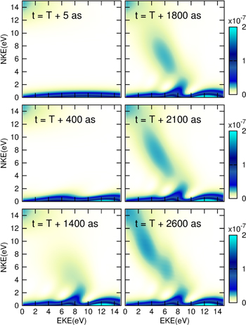
Figure 7. Ionization probability of  , double differential in nuclear kinetic energy (NKE) and electron kinetic energy (EKE) after interaction with a laser pulse with duration
  = 400 as, a central energy of 30 eV, an intensity of
  W cm
W cm and with polarization along the nuclear axis. Each panel corresponds to a snapshot of the double differential ionization probability at a given time t
  T up to
  = 3 fs for the last panel. The fingerprint of the decay of the lowest
  DES is observed in its time-resolved leaking into the electronic continuum in channel
  .
.
Download figure:
Standard image High-resolution imageFor times t  T, we observe the onset of ionization signals leading to nuclear fragments with higher energies (and less energetic electrons). This is due to the autoionization process that is governed by the NWP moving into the DES potential energy curve (PEC). These DES are purely dissociative and, consequently, the NWP moves in the PEC toward larger internuclear distances, thus accumulating nuclear momentum (i.e., more energetic nuclear fragments). Since the total available energy
  has to be shared between nuclei and electrons, and autoionization eventually takes place at a given internuclear distance, electrons are ejected with lower kinetic energies as the NWP proceeds into the dissociative region. When both the DES and the continuum are excited by the laser pulse, we observe in figure 7 the build-up of energy-dependent patterns that are the signature of the interference between direct ionization and the delayed autoionization from the DES. Most observed features can be understood and reproduced by means of semiclassical models as discussed in [79, 123]. The converged asymptotic limit is already reached in our calculations for a time t
  +2600 as = 3 fs (last panel in figure 7), which is approximately equal to the lifetime of the lowest (and the only efficiently excited) DES in the
  series of
  symmetry. For larger evolution times the probabilities remain unchanged. Note that any experiment using a single pulse will only capture this long-time limit of the photoionization distribution unless a time-delayed laser probe is introduced to record the short-time dynamics.
Also notable in figure 7 are the wide EKE distributions at low NKE in comparison with the narrower signal coming from autoionization, inasmuch as the Fourier transform of the short pulse leads to a much wider frequency spectrum. This is explained by the bound/continuum character of the states: in direct dissociative photoionization, one reaches a double continuum resulting from nuclear dissociation and electron ionization, so that there always exists a vibronic state with energy  (NKE+EKE) for each frequency component
  (within the bandwidth of the pulse) that fulfills the energy conservation law NKE+EKE=
 . The autoionization signal comes instead from a NWP that moves in a discrete state (the lowest
  DES); therefore only those DES vibrational energies lying within the Franck–Condon region are excited by the pulse, no matter what its duration. Each photon frequency
  must thus obey
  , where
  is the potential energy curve of the DES,
  = 1.4 a.u. is the equilibrium distance of the
  molecule and
  R is the width of the Franck–Condon region, as plotted in figure 6. Consequently, for very short pulses, the direct photoionization signal is delimited in total energy by the energy bandwidth of the pulse (assuming that the dipole transition moment between the ground and the electronic continuum states, equation (15), varies smoothly within the energy range of interest), while the autoionization bandwidth is mostly dictated by the Franck–Condon region.
For longer pulse duration, as shown in figure 8, the ionization distributions run along the diagonals given by the function NKE= EKE and they are now clearly determined by the smaller width of the laser pulse in both the direct and the autoionization regions. In this second example, we use pulses of 1 and 10 fs duration. Also, we have slightly increased the central photon energy to 33 eV to ensure that the
  series of DES, as well as the continuum corresponding to the second ionization threshold
  , are reached. The intensity is set to
  W cm−2 , although its value is irrelevant, since for one-photon processes the modification of the intensity only affects probabilities through a global scaling factor (see equation (52)). The use of a monochromatic source (like in synchrotron radiation, and for practical purposes a duration
  = 10 fs satisfies this condition in the present example) carries a single value of
  that implies that, for a given energy sharing, there only exists a unique pair (NKE,EKE) satisfying total energy conservation. In such a case, the same information is extracted from doubly differential ionization probabilities in (NKE,EKE) or singly differential in NKE or EKE (the latter two would be mirror images). For short pulses (non-monochromatic light) this is no longer true, because the singly differential quantities in NKE (or EKE) result from the integration over EKE (or NKE), implying that one is losing part of the information contained in the doubly differential probabilities. Still, for each individual diagonal line given by a particular frequency
  within the bandwidth of the pulse, i.e. NKE=
 EKE, the singly differential probabilities in NKE and EKE are mirror images, but this symmetry breaks down due to the averaging over all frequencies when integration is performed over EKE (or NKE). The same result shown in figure 8 can be extracted by using synchrotron radiation and performing a fine scan of photon energies [71]. The spectrum for short laser pulses (
 = 1 fs in figure 8) can be thus reconstructed by normalizing, at each frequency
  , the resulting synchrotron radiation correlated spectra (NKE,EKE,
  ) with the square of the Fourier transform of the pulse.

Figure 8. Ionization probability of  , double differential in nuclear kinetic energy (NKE) and electron kinetic energy (EKE) for a laser pulse with central frequency 33 eV, intensity
  W cm
W cm using two different pulse durations:
  = 1 and
  = 10 fs.
Download figure:
Standard image High-resolution imageIn attosecond studies on molecular targets, it is not always possible to detect all particles in coincidence. In fact, it is common to measure only the ejected ions (or the ejected electrons). In this case, one would be measuring the singly differential probabilities as in figure 9, corresponding to the doubly differential probabilities in figure 8 integrated over the EKE axis. When using nearly monochromatic radiation (10 fs pulse), we observe in the NKE distributions of figure 9 an oscillating pattern due to the interference between the direct and the autoionization pathways, whereas for the 1 fs pulse the integration over such large energy bandwidth smoothes out these structures. To illustrate that the loss of information in the integrated probabilities when short (1 fs) pulses are used is entirely due to spectral effects, we make use of the first order TDPT for the doubly differential probabilities by using the expression (52) and then relate the probabilities calculated for two different pulse durations  . One arrives at the formal identity
where  is given in equation (53). The result obtained from equation (60), also plotted in figure 9, perfectly matches the probabilities for the 10 fs calculation. Obviously, the same kind of identity cannot be applied if only NKE (or EKE) are measured when one uses short pulses [86]. This explains why, for a proper extraction of the total dissociative photoionization cross-sections, one has to measure either doubly differential probabilities (when using short pulses) or singly differential probabilities (when using very long pulses).

Figure 9. Nuclear kinetic energy (NKE) distributions: ionization probabilities integrated over electron energy and plotted as a function of NKE. All results are computed for pulses centered at 33 eV and with an intensity of 10  W cm
W cm . Solid black line: TDSE results for a 1 fs pulse. Dashed black line: TDSE results for a 10 fs pulse. Circles: 10 fs results obtained through equation (60) from the solution of the TDSE using the 1 fs pulse. Colored dashed lines correspond to the contributions from the 1s
 and the 2p
 ionization channels to the total dissociative ionization for the 10 fs pulse. Note that for comparison, we have renormalized the probability with the pulse duration. The dotted vertical lines indicate the NKE values for which angular distributions are plotted in figure 10.
Download figure:
Standard image High-resolution imageAs mentioned in the theory section, measurements that determine the ejection angle of the particles can give a deeper insight into the electron and nuclear dynamics. In fact, some information is only encoded in the angular distributions, as e.g. the molecular symmetry components [22]. The angular distributions, equation (46), for dissociative photoionization induced by a 33 eV pulse of 10 fs duration are plotted in figure 10 for three particular energy sharing pairs (NKE,EKE) with total available energy NKE+EKE = 14.92 eV (the selected NKE values are also indicated in figure 9). In figure 10(a) we take an energy sharing (2 eV, 12.92 eV) for which only the lowest ionic state  is populated by direct ionization. In figure 10(b) we plot an energy sharing (12.6 eV, 2.32 eV) where a small ionization contribution from the second lowest ionization threshold
  is present along with ionization into the first ionic state
  coming from autoionization. Finally, in figure 10(c) we plot the angular distribution for an energy sharing (14.8 eV, 0.12 eV) where we again have contributions from both ionic states, but with a larger contribution from the second ionization threshold. As theoretically demonstrated in previous works [71, 124–126], an asymmetry in the electron ejection is expected to appear in the context of dissociative photoionization of homonuclear molecules as a result of the coherent superposition of states with different inversion symmetry (gerade and ungerade). The temporal build-up of the molecular frame angular distributions is included in figure 10, where in particular panels (b) and (c) show the formation of a prominent asymmetry in the electron ejection with respect to the proton release due to the coherent contribution of the two ionic states, while panel (a) shows a perfectly symmetric electron ejection at any time. Right at the end of the interaction with the ulstrashort pulse (for times t = T = 1 fs and even for
  +1 fs = 2 fs), all angular distributions are symmetric regardless the energy sharing we are considering. For those short times, the delayed autoionization process has not yet occurred and direct ionization releases electrons with very different kinetic energies in the
  and
and  channels. This precludes any interference between them and, consequently, the angular distribution of the ejected electrons is completely symmetric. As the DES decay into the
  ionization continuum while the molecule dissociates, electrons (and protons) can be ejected with the same energy as those in the
  direct channel. Hence the two different paths can interfere coherently, leading to the observed asymmetry. Note that, 3 fs after the end of the pulse, convergence of the angular distributions to their asymptotic limit is already reached. Sophisticated experimental works have demonstrated the suitability of using the symmetry breaking of the electron ejection as an strategy to map electron and nuclear dynamics in small molecules. These works have been performed with IR pump–IR probe schemes, where electron localization is achieved by controlling the relative CEP between the pulses [96, 127–129] or with combinations of a SAP [76] or an APT [130, 131] with IR probe pulses. More recently, some of us have reported a theoretical prediction using the present methodology, showing how, by using a UV pump–UV probe scheme, the asymmetry in the electron angular distributions maps the motion of the NWP associated to excited states of the molecule [22].
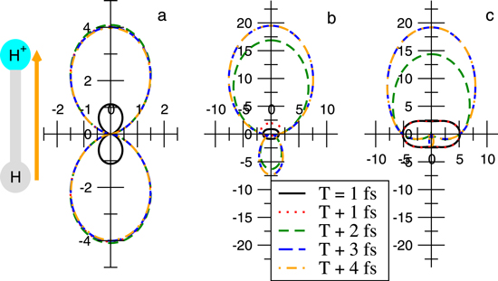
Figure 10. Fully differential ionization probabilities in 10 (differential in nuclear and electron kinetic energies and in electron ejection angle) at different times after the pulse (1 fs, 33 eV and 10
 W cm
W cm ) is turned off. We pick for all panels a total final energy of 14.92 eV (NKE+EKE), where the maximum probability appears. (a) NKE = 2 eV and EKE = 12.92 eV; (b) NKE = 12.6 eV and EKE = 2.32 eV; and (c) NKE = 14.8 eV and EKE = 0.12 eV. The proton ejection direction (upward) and the light polarization direction (yellow arrow) are indicated on the left side.
Download figure:
Standard image High-resolution imageFor a better comparison with actual experiments, a more integrated quantity is usually defined, the asymmetry parameter. It simplifies the measurement (increasing the number of counts) while still quantifying the symmetry/asymmetry degree in the electron ejection. The asymmetry parameter is defined as (assuming the geometry shown in figure 10):

where  is the probability of ejecting an electron upwards (downwards).
  is evaluated by integrating the electron angular distribution over the solid angle in the two hemispheres separated by the plane that contains the inversion center and is perpendicular to the molecular axis. In the examples discussed below, we compute
  for proton ejection along the laser polarization axis. This is usually known as molecular-frame asymmetry, because it is measured with respect to the proton ejection direction, which coincides with the molecular axis.
In figure 11, we plot the asymmetry parameter as defined in equation (61) (doubly differential in NKE and EKE) corresponding to the results shown in figures 8–10 for the 1 fs pulse and in the energy region where only one-photon transitions are possible. From equation (60), we know that this result is independent of the pulse duration. The exact same features shown in figure 11 can be extracted from an energy scan with synchrotron radiation [71], from an isolated ultrashort pulse or from an APT [132]. Obviously, this statement strictly applies as long as only one-photon transitions are considered and the stationary regime has been already reached [85, 133]. If a second radiation source is introduced, like an IR pulse that overlaps in time with the former pulses [76, 134] or a second time-delayed UV pulse [22], quite different features, encoding the initially pumped dynamics, would be obtained. A brief review of these UV+IR and UV+UV problems in the context of our spectral TDFCC methodology will be given in 6.

Figure 11. Ab initio calculation for the asymmetry parameter for electron emission in dissociative ionization after one-photon absorption from the ground state. The asymmetry occurs when both ionization thresholds lead to fragments with the same final energies: the 1s  —through the decay of the
  DES of
  symmetry—and the 2p
  —through direct photoionization.
Download figure:
Standard image High-resolution image5. Laser polarization effects: circular dichroism in photoionization of

All the results presented above were obtained for linearly polarized light parallel to the molecular axis. However, the choice of the polarization direction of the laser field and its orientation with respect to the molecular axis has a substantial impact on the photoionization outcome [71]. In fact, one of the most striking effects is the presence of a net circular dichroism (CD) in the photoionization of  , which is a nonchiral molecule (since it has a center of inversion) and therefore does not exhibit optical activity [73, 135]. Circular dichroism in the angular distributions (CDAD) corresponds to the difference in the photoionization cross-sections, differential in the emission polar angle
  relative to the molecular axis (see figure 12), resulting from two different helicities
  (left-handed circularly polarized light) and
  (right-handed circularly polarized light). In this case, the required handedness for the optical activity comes from the enantiomorphic arrangements induced by the photon–molecule system when considering the relative orientations of the vectors associated to the molecular orientation
  , the direction of photoelectron momentum
  and the direction of the light propagation
  in figure 12. The non-coplanar orientation of the triplet of vectors
  is a necessary condition for the CDAD to exist [136, 137]. These findings have been possible with the detailed analysis of molecular-frame photoelectron angular distributions (MFPAD) in dissociative photoionization experiments in which the orientation of the molecule in gas phase is fully determined (fixed-in-space molecules) at the time of photon impact. This information is available from multicoincidence detection techniques (COLTRIMS) [99] or vector correlation methods [138, 139], in which the full momentum of all ejected charged particles is determined from the measurement in coincidence of ejected protons and electrons in each dissociative ionization event. In [73, 135] some of us showed that CDAD only occurs at proton kinetic energies where both the
  ionization channels are open, a condition that requires photon energies above 30 eV, from which the
  ionization channel is energetically open. As an illustration, figure 12 shows the contributions to the dissociative ionization spectrum from both ionization channels at a photon energy of 32.5 eV. As can be seen, the
  contributions overlap at proton kinetic energies larger than 3.5 eV. At such proton kinetic energies, the forms of the MFPAD (see figure 12) and the CDAD are almost entirely determined by the autoionization from the
  doubly excited states of
  (see figure 6). In contrast to linearly polarized light (for instance, the NKE distributions shown in figure 9 for
  = 33 eV and linear polarization along the molecular axis), one-photon absorption with circularly polarized light (
 = 32.5 eV) ionizes
  , leading to final continuum states with both
  (parallel transitions to states with
  = 0) and
  (perpendicular transitions to states with
  = 1) symmetries. This implies that photoelectrons in the H
 channel are ejected with odd values of angular momentum
  and with
  = 0 (
= 0 ( ) and
) and  , and that they interfere with those ejected from the H
 channel with even values for
  and also with
  , ±1. In addition, since in these types of experiments the proton is detected in a given direction, this localization condition must be implemented with linear combinations of the asymptotically degenerate ionic states
  , as explained in the theory section.
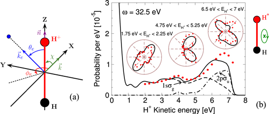
Figure 12. (a) Photoionization axis frame. The  molecule is oriented along the
  -axis. The light propagation direction is represented by the vector
  along the
  -axis, so that the polarization vector rotates in the YZ plane. The electron is ionized in the direction given by
  and has a momentum vector
  . The proton is ejected in the upward direction
  along the molecular axis
  . (b) Proton kinetic energy and electron angular distributions. Dissociative ionization probability in
  as a function of the proton kinetic energy for left-handed circularly (LHC) polarized light (or helicity
  ) for a photon energy
  = 32.5 eV. Red circles, experimental results; black solid line, theoretical results; black dashed line, contribution to the dissociative ionization probability from the
  ionization channel; black dash-dotted line, contribution from the
  channel. Insets: polar plots of the molecular-frame photoelectron angular distributions in the
  plane (i.e.
  in (a)) at fixed proton kinetic energies averaged within the energy intervals indicated in the figure. Same notation as for the probabilities.
Download figure:
Standard image High-resolution imageThe molecular-frame photoelectron angular distributions (MFPAD)  displayed in figure 12(b) for the geometry shown in figure 12(a) are those corresponding to electron emission in a plane
  perpendicular to the light propagation axis (
 = 90° or 270°) and containing the molecular axis (
 = 90°), and only for the selected left-handed circularly (LHC) polarized light of positive helicity
  = +1. MFPADs in this geometry can be parametrized according to the expression [140, 141]
where the geometrical dependence on the azimuthal angle  is factorized in terms of simple trigonometric functions, and the dynamical information on the dissociative ionization process is fully contained in four
  functions, whose explicit expression can be found in [135] (see also [118] and [142]). In the
  plane, the CDAD corresponds to the relative variation of the MFPAD
  when the helicity of the light is changed from
  = +1 (LHC) to
  = −1 (RHC), which in turn can be also defined in an equivalent form involving only one helicity (
 = +1 for instance) as follows

or in terms of the  functions as
  , showing that the
  function is the driving factor responsible for CDAD. By using the values of the MPPADs at
  = 90° and
  = 270°, which can be extracted from figure 12(b), one can easily evaluate the value of the CDAD for each value of
  by using equation (63). One immediately realizes that CDAD(
 ) is almost an antisymmetric function in the interval
 ![${\theta }_{e}\in [0,{180}^{o}]$](https://content.cld.iop.org/journals/0953-4075/48/24/242001/revision1/jpb518094ieqn801.gif) in the proton kinetic energies intervals
in the proton kinetic energies intervals ![${E}_{{H}^{+}}\in [1.75,2.25]$](https://content.cld.iop.org/journals/0953-4075/48/24/242001/revision1/jpb518094ieqn802.gif) eV (leftmost distribution) and
eV (leftmost distribution) and ![${E}_{{H}^{+}}\in [6.5,7]$](https://content.cld.iop.org/journals/0953-4075/48/24/242001/revision1/jpb518094ieqn803.gif) eV (rightmost distribution). By contrast, MFPADs in the interval
eV (rightmost distribution). By contrast, MFPADs in the interval ![${E}_{{H}^{+}}\in [4.75,5.25]$](https://content.cld.iop.org/journals/0953-4075/48/24/242001/revision1/jpb518094ieqn804.gif) eV display very different patterns, so that CDAD(
eV display very different patterns, so that CDAD( ) does not exhibit any particular symmetry with respect to the polar emission angle
  . Since the net circular dischroism (CD) is defined by integrating over the latter angle, i.e.,

departures from the typical antisymmetric behavior of CDADs with respect to  can be experimentally determined when the measured CD is different from zero. Indeed, figure 13(a) shows that the measured CD in
  for a photon energy of 32.5 eV clearly departs from zero for protons with kinetic energy
 ![${E}_{{H}^{+}}\in [4,6]$](https://content.cld.iop.org/journals/0953-4075/48/24/242001/revision1/jpb518094ieqn809.gif) eV, in good agreement with theoretical calculations [73].
eV, in good agreement with theoretical calculations [73].
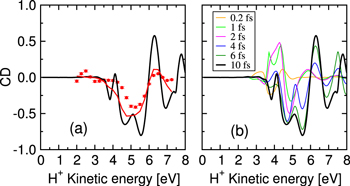
Figure 13. Effective circular dischroism (CD) related to the MFPADs included in figure 12(b), for a photon energy of 32.5 eV. (a) Red dots, experimental results; black solid line, theoretical results; red solid line, theory convoluted with the experimental resolution in energy and solid angle. (b) Temporal build-up in ![$t\in [0,T]$](https://content.cld.iop.org/journals/0953-4075/48/24/242001/revision1/jpb518094ieqn810.gif) of the calculated CD up to the total duration of the laser pulse
of the calculated CD up to the total duration of the laser pulse  = 10 fs.
Download figure:
Standard image High-resolution imageFigure 13(b) also shows the calculated time evolution of CD for a laser pulse with a duration  = 10 fs. The presence of CD is the clear fingerprint of the interferences among different ionization channels of different inversion symmetries (
 ) due to the resonance decay of
  doubly excited states occurring at different time delays. At very short times (
 fs), autoionization from the
  resonances, which are those most abundantly populated, has not yet taken place and, consequently, the MFPADs yield a CDAD function which is antisymmetric with respect to
  = 90°, and thus CD is practically zero for all proton kinetic energies. In the interval t
 ![$\in \;[1,2]$](https://content.cld.iop.org/journals/0953-4075/48/24/242001/revision1/jpb518094ieqn819.gif) fs, major changes in the CD appear, in particular, oscillations at proton kinetic energies
fs, major changes in the CD appear, in particular, oscillations at proton kinetic energies ![${E}_{{H}^{+}}\in [3,5.5]$](https://content.cld.iop.org/journals/0953-4075/48/24/242001/revision1/jpb518094ieqn820.gif) eV. These oscillations reflect the early stages of the autoionizing decay from the
eV. These oscillations reflect the early stages of the autoionizing decay from the  resonances into the ionization channels
  , respectively. In the time window t
 ![$\in \;[4,6]$](https://content.cld.iop.org/journals/0953-4075/48/24/242001/revision1/jpb518094ieqn823.gif) fs, the delayed decay from the
fs, the delayed decay from the  resonance into the lowest ionization threshold
  comes into play, thus leading to oscillatory patterns at higher proton kinetic energies,
 ![${E}_{{H}^{+}}\in [5.5,8]$](https://content.cld.iop.org/journals/0953-4075/48/24/242001/revision1/jpb518094ieqn826.gif) eV. All these findings suggest that the onset of circular dischroism in homonuclear diatomic molecules could be used as a sensitive probe to scrutinize the fast dynamics associated to molecular autoionization.
eV. All these findings suggest that the onset of circular dischroism in homonuclear diatomic molecules could be used as a sensitive probe to scrutinize the fast dynamics associated to molecular autoionization.
6. Pump–probe schemes
6.1. Two-color (UV–IR) Pump–probe
In 2009, UV-pump/IR-probe experiments were performed to track dissociative photoionization of  and D
and D using femtosecond pulses, which allowed the investigation of the NWP dynamics associated to field-dressed ionic states [143]. One year later, the faster electron dynamics associated to excitation in the region of the D
 autoionizing states was explored in a similar two-color UV–IR scheme, but now using an isolated attosecond UV pulse as the pump [76]. While in the first problem the theoretical description can be achieved by simply considering the NWP moving in a one-dimensional PEC, an accurate description of the second one mandatorily requires treating both electronic and nuclear motion. As we discussed in detail in sections 4 and 5, autoionization from DES and nuclear motion occur in a similar timescale, and consequently electronic and nuclear motions must be coupled during the time propagation. However, the addition of an IR field considerably complicates the picture with respect to the physics shown in the two previous sections, often accompanied by a significant increase in the computational effort. Indeed, an electron excited to the continuum by the UV pulse can absorb IR photons (above threshold ionization), thus gaining both energy and angular momenta. The former implies the use of larger radial boxes and denser grids, and the latter a dramatic increase in the number of partial waves included in the angular expansion of the wave function. The introduction of a full set of dipole couplings between continuum states of different symmetries (for instance,
  for linear polarization along the molecular axis), in order to represent these above-threshold IR transitions, comes with the cost of including double sets of electronic and vibrational continua for each ionization threshold of H
 . In spite of these additional complications, the huge improvement in computational capabilities in the last few years, e.g., by means of supercomputers, have made it possible to perform the first calculations considering molecular ionization by broadband UV pulses combined with IR fields.
In 2010, the combination of these theoretical efforts with a pioneering experiment that made use of an isolated UV attosecond pump pulse and an IR fs probe pulse demonstrated the possibility of controling the localization of the electronic charge within the molecule as it dissociates [76]. In this specific UV–IR scheme, a single attosecond pulse of 300--400 as centered at 30 eV, whose spectrum extends from 20 to 40 eV, was used to trigger a prompt ionization. Such a bandwidth covers a wide range of energies, thus leading to population of the first two ionization continua and the first series of  DES (see the energy diagrams plotted in figure 14). In the absence of the IR radiation, the angle- and energy-differential ionization probabilities follow the patterns discussed in section 4. However, when the UV pulse is combined with a time-delayed intense IR pulse with the same linear polarization and a FWHM of 6 fs, a laboratory-frame symmetry breaking is observed. To quantify this effect, the experiments aimed at determining the asymmetry parameter, which is formally defined as in equation (61), but with an important difference: at variance with the molecular-frame asymmetries measured in one-photon ionization [71, 86] and discussed in section 4, laboratory-frame asymmetries are determined by considering all electrons ejected in a given direction with respect to the polarization vector, regardless of the proton ejection direction. The dependence of the calculated asymmetry parameter with respect to the proton kinetic energy and the time-delay between the UV and the IR pulse is plotted in figure 14. The time-delay is defined as the elapsed time between the centers of each pulse. Two main mechanisms, labeled mechanism I and II in the figure, were identified as being responsible for the asymmetry. In mechanism I, the asymmetry comes from the interference between autoionization into the lowest molecular ionic state
  and direct photoionization by the combined action of UV+IR photons. Mechanism I is thus observed for the shortest time delays, when the pulses efficiently overlap in time, favoring the simultaneous absorption of a UV and an IR photon. In mechanism II, there is a laser-induced transition from the
  state of
  (resulting from ionization of
  by the UV pulse) to the
  state of
  . This is a sequential process in which the NWP created by the UV pulse in the ground state of
  moves until the IR pulse couples it to the first excited ionic state through absorption of a few IR photons. This mechanism can thus be observed even when the pump and probe pulses do not overlap.

Figure 14. Upper panels: illustration of two different quantum paths responsible for the observed electron asymmetry in two different regions of time delays. Bottom left: asymmetry in dissociative photoionization of  subject to a UV–IR protocol. The asymmetry parameter is plotted as a function of the proton kinetic energy and the pump–probe delay, integrated over all possible electron energies. Bottom right: schematic representation of the processes related to each mechanism (I and II). See text for details.
Download figure:
Standard image High-resolution imageIt is worth stressing that the molecular-frame asymmetry discussed in 4 is strictly due to one-photon absorption processes. It results from the interference between two dissociative paths that involve ionic states of different inversion symmetry (gerade and ungerade) and electrons with different angular momenta, i.e., continuum states of the type { *
* } and {
 *
* }. The laboratory-frame asymmetry described here also involves ionic states of difference inversion symmetry, but at variance with molecular-frame asymmetries, they involve electrons with the same angular momentum. This possibility arises from continuum–continuum
  ↔
↔ transitions induced by the IR field, which open ionization channels of the form {
 *
* } and {
 *
* } (see [144, 145]).
The proposed mechanisms are confirmed by the NKE distribution as defined in equation (43), i.e., integrated over all the electron ejection angles and energies, and plotted as a function of time delay. Their role has been made evident in more recent calculations using other laser parameters. For instance, the result of an equivalent UV-pump/IR-probe calculation is plotted in figure 15. Specifically, we now use a single attosecond pulse (SAP) (with 400 as of FWHM), centered at 28 eV and intensity  =
=  W cm−2 and a 750 nm IR pulse (∼1.65 eV) with duration 9 fs and
  W cm−2. The calculated total NKE distributions for the dissociative ionization channel are shown in figure 15(a). Panels (b) and (c) show the contributions from each final symmetry: (i)
  (optically allowed with the absorption of an odd number of photons from the ground state X
 ) and (ii)
  (with the absorption of an even number of photons from the ground state or an odd number of photons from the previously populated
  continuum). In panels (d)–(f) and (g)–(i) the contribution of the 1s
 and 2p
 ionization thresholds is shown separately. For negative time-delays (the IR reaches the target before the SAP), the distribution is identical to that obtained when only the UV pulse is present, because the number of IR photons required to reach the lowest ionization limit H
 from the ground state in the Franck–Condon region is around ten, which is not possible at the IR intensities used in these calculations. For time delays at which the UV and the IR pulses effectively overlap, between approximately −4 to 4 fs, the NKE distribution signal oscillates with half the period of the IR. This is a rather expected behavior, as shown by a number of recent UV+IR experiments, and is the signature of the so-called laser-assisted photoionization [76, 134, 146, 147]. However, in our problem the modulation with the IR is not strictly symmetric with respect to zero time delay because autoionization breaks this symmetry [76]. This is evident in panels (g)–(i), where the NWP moving in the DES favors a sequential process that leads to fragments into the 2p
 ionic state at NKE in the interval 10–15 eV. These same panels also show the fingerprint of mechanism II discussed above (see figure 14(b)). At time-delays larger than 4 fs, a strong ionization signal appears in the second ionization threshold for low NKE. This reflects the fact that the NWP, initially created by the UV pulse in the
  state of
  and subsequently evolved in time, is strongly coupled to the excited
  state of
  by the IR field when the NWP reaches an internuclear distance of about 3-4 a.u., which is the farthest it can go in 4 fs. This effect was described many years ago and is known as bond-softening [148–150].
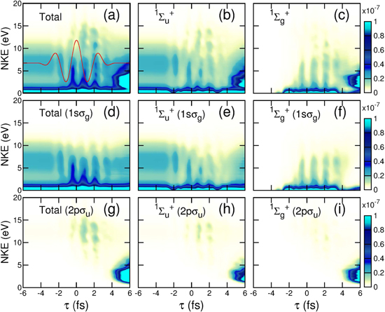
Figure 15. Dissociative photoionization probability as a function of nuclear kinetic energy (NKE) and time delay  between the UV and the IR pulses. UV pulse parameters:
  = 28 eV,
  =
=  W cm
W cm = 1 fs (FWHM of 400 as). IR pulse parameters:
  = 1.65 eV,
  W cm
W cm = 9 fs. (a) Total photoionization probability. (b) Partial contribution leaving the ionized system in a
  symmetry. (c) Partial contribution leaving the ionized system in a
  symmetry. (d) Partial contribution associated with the ionic state
  . (e) Partial contribution associated with the ionic state
  within the
  symmetry (i.e. an odd number of photons absorbed). (f) Partial contribution associated with the ionic state
  within the
  symmetry (i.e. an even number of photons absorbed). (g)–(i) Same as in (d)–(f), but associated with the first excited ionic state
  . The magnitude of the vector potential
  of the IR laser centered at
  = 0 is also included in (a) as a red line.
Download figure:
Standard image High-resolution imageA different, widely studied problem, in which overlapping attosecond UV and moderately intense fs IR pulses are used, is electron streaking [151–153]. In streaking, the momentum or kinetic energy of the emitted electron is recorded as a function of the time-delay between the UV and the IR pulses. This technique, mostly applied to atomic systems, is commonly used to elucidate the optical characteristics of a SAP from a structureless photoelectron spectra. However, one can use it the other way around to elucidate the target structure from the streaking patterns induced by a known laser pulse. Figure 16 shows the calculated EKE distributions for  as a function of time delay. For analysis purposes, we superimpose the values of minus the IR vector potential,
  (t), in both panels.

Figure 16. Electron kinetic energy (EKE) distributions as a function of the time delay  between UV and IR pulses (same laser parameters as in figure 15) for an ejection angle 0° with respect to the polarization vector, which is parallel to the molecular axis. Left: total photoionization. Right: dissociative photoionization (note the different scales); dissociation is less than 10% of total ionization, consequently autoionization clearly manifests in this channel by strongly modifying the streaking pattern. The negative value of the vector potential magnitude
 ![$[-{A}_{{IR}}(t)]$](https://content.cld.iop.org/journals/0953-4075/48/24/242001/revision1/jpb518094ieqn889.gif) is also included with a red line.
is also included with a red line.
Download figure:
Standard image High-resolution imageIn the streaking technique, as described for atomic targets, the UV pulse is much shorter than the IR pulse and one can thus consider the photoelectron being emitted at a well-defined time delay. The photoelectron momentum recorded in time follows, within a simple classical approximation, the vector potential of the IR field,  (t) such that,
  , with
  being the electron momentum at the instant of ejection. Note that in figure 16 we have only included photoelectron emission for an angle 0° with respect to the polarization vector (aligned with the molecular axis). That is to say, we have plotted the result of equation (44) before integrating over a solid angle. Electron emission at angles different from 0° (or 180°) would require to consider geometrical effects that are ignored in a classical picture [154]. The interaction with the remaining ion is also fully neglected in the classical picture, although other extended models can include it to a given extent [155]. Nevertheless, as can be seen in the left panel of figure 16 (labelled 'Total') the probabilities match the expected classical streaking pattern. The left panel shows the total photoionization probability, which in this case includes all dissociative and non-dissociative channels, i.e. it is the probability that results from integrating over all nuclear continuum states and summing over the bound vibrational states associated to each H
 ionic state. In the right panel of figure 16, we plot instead only the dissociative photoionization contribution, where we observe a rather modified signal due to the larger contribution of autoionization that produces electrons at different times and energies. Again, we observe that probabilities are not symmetric with respect to zero time delay. For negative delays, the probabilities follow the streaking patterns that correspond to electrons moving in a structureless continuum, which is compatible with the fact that only direct ionization is possible. By contrast, for positive delays the signature of autoionization complicates this pattern. Further investigations are needed to explore the possibility of extracting the ionization times from such streaking signal. In fact, studies on electron streaking in molecules are still very scarce and only very recent works seek to explore the effect of a multi-center target in the expected photoionization time-delay [156–158].
6.2. One-color UV-pump UV-probe
We now explore pump–probe schemes in which only UV radiation with relatively low intensity is used. Due to the large value of the corresponding Keldysh parameter, this UV radiation excites and ionizes the  molecule without perturbing the Coulomb potentials that the particles feel. In this way, the probe step provides information about the intrinsic molecular dynamics of the system and not about the dynamics induced by the probe itself. This is important because in all the UV+IR probe schemes discussed above, most of the observed dynamics is induced by the intense IR pulse, which somewhat hides the field-free intrinsic dynamics of the system, e.g., autoionization.
The first UV pump–UV probe experiments reported in the literature made use of two identical ultrashort pulses of few tens of femtoseconds generated by the free-electron laser in Hamburg (FLASH), and the chosen targets were  and
and  [74, 75]. The sequence of the two UV pulses leads to double ionization of the molecule: the first pulse ionizes
  , inducing NWP dynamics in the ground state of
  and the second pulse maps the NWP motion into the proton kinetic energy spectra resulting from the Coulomb explosion of the molecular ion following the removal of the second electron. In these pioneering experiments, the time resolution was slightly below 10 fs, which was enough to explore the ratio between direct and sequential double ionization processes.
In general, the available x-ray free-electron laser facilities (such as FLASH in Hamburg, LCLS at Stanford, and others) are already able to produce intense XUV pulses, but the shortest pulse durations that they can provide are of the order of a few fs [159], which is still too long to obtain a clean picture of electron dynamics. At present, the most suitable alternative is to use UV or XUV pulses resulting from HHG processes, as explained in the introduction. In fact, the first experimental attempts using XUV-pump/XUV-probe protocols to retrieve electron dynamics in atoms [160] and in the hydrogen molecule [21] were performed recently using HHG techniques that achieve a time resolution of the order of 1 fs. These works measured the total ionization signal as a function of the time-delay between the two pulses, whose Fourier analysis partly reveals the frequencies involved in the pumped target in good agreement with theoretical simulations. Following these works, full dimensional ab initio theoretical calculations performed on He [161] and  [22, 77] made use of interferometric schemes based on the use of replicas of attosecond UV pulses that allow one to trace the time evolution of electron wave packets. In particular, in a recent theoretical work on
  [77], some of us showed how the amplitudes and phases of the vibronic (vibrational+electronic) wave packet that is created by the pump pulse can be extracted from the total ionization probabilities. The XUV-pump/XUV-probe scheme used in [77] is shown in figure 17, which we discuss briefly below.

Figure 17. Energetics of the XUV-pump/XUV-probe scheme with twin 2 fs pulses ( = 12.2 eV and
  =
=  W cm
W cm ) with a time delay
  = 6 fs between them. The absolute squared value of the Fourier transform of the 2 fs pulse is plotted in the y-axis on the left panel, showing the relatively large energy bandwidth of the pulses. The relevant potential energy curves (electronic states) are labeled in the figure: the ground state (X
  ), the two lowest excited states
  (B and B'), the lowest
  doubly excited states and the two lowest ionization thresholds 1s
 and 2p
 . The blue shaded areas represent the NWPs generated by the pump pulse at the times indicated in the figure: (a) t = 2 fs; (b) t = 4 fs; and (c) t = 8 fs. The red shaded areas represent the NWPs generated by the probe pulse absorption from the ground state at t = 8 fs. The green shaded area represent the NWP generated by the probe pulse absorption from the evolving NWP. The scheme with the pump and probe pulses separated by τ = 6 fs is drawn in (d). The orange arrows represent direct two-photon ionization by the pump and probe pulses, and the green arrow represents the absorption of a single photon from the probe pulse after free evolution of the NWP generated (sequential two-photon ionization process). The black curves superimposed to the blue and red NWPs in (c) represent the NWP resulting from the interference between the red and blue NWPs.
Download figure:
Standard image High-resolution imageIn this scheme, we use two identical UV pulses of 12.2 eV (or 14 eV) and 2 fs total duration, and intensities of 1012 W cm−2. A plot of the twin pulses in the time and frequency domains is shown in figures 3 and 4. We scan the ionization probabilities for time delays from 0 to 100 fs, thus accounting for the longest oscillatory periods of intermediate vibrational states that can be populated by the pump pulse, namely those associated to the electronic singly excited states B and B'  in H2 [21]. As described in section 4, among the possible ionization events we have both dissociative and non-dissociative direct photoionization as well as autoionization from the lowest series of
  DES. In the present UV–UV problem, however, only the
  DES with symmetry
  are populated, because this is the only symmetry that can be reached in a two-photon transition. Note that ionization yields are rather large since absorption of the first photon to the B and B' states is a resonant process (see figure 17).
Figure 17 shows that the first pulse can both excite H2 through a one-photon transition and ionize it through a two-photon transition. More explicitly, the pump pulse produces a molecular wave packet associated to the B and B'  states of H2 and another wave packet in the
  electronic continuum. These two wave packets evolve in time until, after a given time delay, the probe comes. The probe pulse can then create a new wave packet in the
  continuum following one-photon absorption from the B and B'
  states. This wave packet will interfere with that generated earlier in the continuum by the pump pulse. In addition, the probe pulse can also create, in the Franck–Condon region, an exact replica of the vibronic wave packets generated by the pump at time delay zero, as shown in the rightmost panel in figure 17. As in the former case, this will lead to interferences between the wave packets created by the pump and probe pulses. The calculated total dissociative photoionization probability as a function of time delay is shown in figure 18 for two different central frequencies of the twin pulses: 12.2 eV (a) and 14 eV (b). As can be seen in figure 17, photons of 12 eV can only excite the B state of H2, while photons of 14 eV can excite both the B and B'. Thus, it is not surprising that in the second case the interference patterns in the total ionization yields exhibit a more complex structure.

Figure 18. Dissociative photoionization probabilities as a function of the time delay between the twin UV pulses of 2 fs of duration and 1012 W  . (a) Pulse with central frequency
  = 12.2 eV. (b) Pulse with central frequency
  = 14.0 eV. (c) Time series analysis through the Fourier transforms of probabilities in (a) and (b), translated into energies in eV. Along the upper x-axis in (c) we plot the position of the vibronic states associated to the B and the B'
  excited states.
Download figure:
Standard image High-resolution image
For the 12.2 eV pulses in figure 18(a) the ionization yields show a rapidly oscillating pattern superimposed to a slower one. The latter has a maximum at zero time delay (when both pulses overlap in time) and it repeats every 28–30 fs. This time interval is comparable to the averaged vibrational period for the bunch of vibrational states populated by the pump pulse in the B  state. In other words, the slow oscillation pattern reveals the nuclear dynamics associated to the molecular wave packet excited by the pump, and it is visible in the ionization yields because of the mentioned interferences introduced by the two-step process. In this sequential process, one photon from the pump pulse populates a given m intermediate vibronic state, and another photon from the probe pulse is absorbed from the m state to the final continuum states. The interferences between different sequential paths, involving different m intermediate states, reveals the
 ![$\mathrm{exp}[-i({E}_{m}-{E}_{m^{\prime} })t]$](https://content.cld.iop.org/journals/0953-4075/48/24/242001/revision1/jpb518094ieqn927.gif) beatings, which are responsible for the slow oscillations.
beatings, which are responsible for the slow oscillations.
For pulses with energy 14 eV in figure 18(b) the wave packet created by the pump pulse is a coherent superposition of vibronic states associated to the B  and B'
  electronic states. Therefore, the calculated spectrum is not that arising from two disentangled NWPs evolving in different electronic states. To extract the different frequency components, we perform the Fourier transform of the dissociative ionization probability functions (for both 12.2 and 14 eV pulses) and plot them in figure 18(c). We observe that the slow beatings described above are associated to phase differences,
 ![$\mathrm{exp}[-i({E}_{m}-{E}_{m^{\prime} })t]$](https://content.cld.iop.org/journals/0953-4075/48/24/242001/revision1/jpb518094ieqn930.gif) , involving vibronic states of the same (or a few neighboring) electronic states, i.e., vibronic states that differ by 0–2 eV. However, the fast beatings seen in figures 18(a) and (b) are due to phase differences that involve both the ground and the B and B' states,
, involving vibronic states of the same (or a few neighboring) electronic states, i.e., vibronic states that differ by 0–2 eV. However, the fast beatings seen in figures 18(a) and (b) are due to phase differences that involve both the ground and the B and B' states, ![$\mathrm{exp}[-i({E}_{m}-{E}_{0})t]$](https://content.cld.iop.org/journals/0953-4075/48/24/242001/revision1/jpb518094ieqn931.gif) , i.e., energy differences of the order of 11–15 eV. As shown in [77], the complex interference patterns observed in the ionization yield as a function of time delay can be easily interpreted by using the expression:
, i.e., energy differences of the order of 11–15 eV. As shown in [77], the complex interference patterns observed in the ionization yield as a function of time delay can be easily interpreted by using the expression:
where  =
=  is the energy difference between the ground and final states of energies E0 and Ef, respectively,
  =
=  is the energy difference between a given m vibronic (vibrational+electronic) intermediate state of energy Em and the final continuum state, af stands for the two-photon direct ionization amplitude, and bfm is the amplitude for the sequential process, which includes the excitation from the ground to a given m vibronic state and the time-delayed transition from the m state to the final f state. Equation (65) is exact when the following two premises are fulfilled: (i) the ground state remains with a population close to unity at any time and (ii) the probability of absorbing three or more photons is negligible, so that there are no further continuum–continuum/bound transitions from the final state f.
The square of the second term, which describes the sequential process, gives a ![$\mathrm{cos}[({E}_{m}-{E}_{m^{\prime} })\tau ]$](https://content.cld.iop.org/journals/0953-4075/48/24/242001/revision1/jpb518094ieqn936.gif) term (the slow oscillations shown in both figures 18(a) and (b) corresponding to the low energy peaks in figure 18(c)). For 12.2 eV, the beatings associated to
term (the slow oscillations shown in both figures 18(a) and (b) corresponding to the low energy peaks in figure 18(c)). For 12.2 eV, the beatings associated to  only include energy differences between vibrational states associated to the B
  state, then we obtain signals corresponding to the vibrational periods of this state. For 14 eV, we observe in addition those beatings associated to energy differences between vibrational states within the B'
  state, plus the beatings associated to a vibronic state of the B electronic state and a vibronic state of the B' state.
The crossed term between the direct (af) and the sequential process (bfm) resulting from squaring equation (65) leads to a ![$\mathrm{cos}[({E}_{m}-{E}_{0})\tau ]$](https://content.cld.iop.org/journals/0953-4075/48/24/242001/revision1/jpb518094ieqn940.gif) term corresponding to the transition from the ground to the intermediate states. It thus encodes the information about the coupled electron and nuclear dynamics induced by the pump pulse in the latter states (the fast oscillations in the ionization yields). Indeed, the Fourier transform exhibits peaks around 11-15 eV corresponding to each
term corresponding to the transition from the ground to the intermediate states. It thus encodes the information about the coupled electron and nuclear dynamics induced by the pump pulse in the latter states (the fast oscillations in the ionization yields). Indeed, the Fourier transform exhibits peaks around 11-15 eV corresponding to each ![$\mathrm{exp}[-i({E}_{m}-{E}_{0})\tau ]$](https://content.cld.iop.org/journals/0953-4075/48/24/242001/revision1/jpb518094ieqn941.gif) electronic phase, with relative intensities that follow the actual values of the amplitudes that describe the transition
electronic phase, with relative intensities that follow the actual values of the amplitudes that describe the transition  . This can be seen in figure 18(c) where, along the upper x-axis, we have included the energy positions for all m vibronic states, i.e. each vibrational state associated to the B and B' states.
In conclusion, the Fourier analysis of the total ionization yields measured in a XUV-pump/XUV-probe experiment with twin attosecond pulses allows the full reconstruction of the intrinsic coupled electron–nuclear dynamics induced by the pump pulse. The phases and amplitudes of the pumped molecular wave packet can be easily retrieved from the interferometric effects created by the twin pulses and arising from the different quantum paths that involve two-photon direct and sequential processes. Moreover, as discussed in detail in [77], the different electronic and nuclear timescales involved in the dynamics of the pumped wave packet suggest that, by choosing the appropriate time delay between pump and probe, one could favor the transition from a particular electronic state. This is possible because the nuclear dynamics associated to different electronic states comes with different vibrational periods, so that the resulting coherent molecular wave packet still reconstructs at different times in the inner region, thus leading to a selective localization of the wave packet in a particular electronic state. The main conclusions and mechanisms revealed by the pump–probe schemes discussed here for H2, as well as most of the analysis performed in the two previous sections, can be easily extrapolated to other diatomic molecules and probably to larger molecular targets, for which full dimensional theoretical tools are not available at present but experiments can be readily performed.
7. Conclusions and outlook
In this review, we have given an overview of the capabilities of existing state-of-the-art theoretical tools to accurately describe the interaction of femto- and attosecond pulses with simple molecules. Current laser technology already offers the possibility to irradiate matter with relatively intense pulsed radiation in the sub-femtosecond regime, thus opening the way to study electron dynamics in its natural timescale and, eventually, to control such dynamics. Time-dependent theoretical methods are also evolving rapidly in order to understand and shed light on the mechanisms that govern the observed laser-induced phenomena at these short timescales. We have chosen the hydrogen molecule as a benchmark to illustrate the performance of the time-dependent Feshbach close-coupling (TDFCC) method, which has been successfully used in previous works to understand a variety of excitation and ionization processes induced by ultrashort laser pulses. The theory is valid as it is to treat similar problems in other diatomic molecules. The details of the TDFCC method, which are scattered in several previous publications, have been presented in a unified and comprehensive way, so that the reader can better judge its potential for future applications in diatomic molecules, as well as how to generalize it to larger molecular targets. Many of the applications of the TDFCC method discussed here have been developed in parallel to or have been inspired by state-of-the-art experiments, thus providing basic protocols for future experiments. For the sake of completeness, we have also provided an overview of the main characteristics of pulsed radiation in its simplest mathematical form, which has allowed us to emphasize the suitability of time-dependent spectral methods to obtain a physical interpretation of the observed dynamics in terms of potential energy surfaces and couplings between molecular states, i.e., by using the same language as in femtochemistry.
More specifically, within the framework of one- and multi-photon single ionization problems, we have shown the important role of both electron correlation and the coupling between electronic and nuclear motions for the appropriate description of resonant dissociative photoionization of  . The time-delayed decay of doubly excited states, whose description mandatorily requires electron correlation, may eventually yield a temporal asymmetry in the electron ejection. This molecular frame asymmetry results from two interfering ionization paths (prompt direct photoionization and delayed autoionization) that produce electrons with the same energy and angular momenta, but leave the residual target in ionic states of different inversion parity. In a further step, we have used light that combines different polarization orientations with respect to the molecular axis and found that, in particular cases, the resulting asymmetries in the electron angular distributions are responsible for the unexpected presence of circular dichroism in the hydrogen molecule. These phenomena associated to electron localization and asymmetries in the electron ejection have been demonstrated experimentally, both with linearly polarized and circularly polarized light, as well as theoretically explained using the time-dependent methodology presented here.
We have also presented a summary of the widely used UV-pump/IR-probe schemes to explore electron dynamics in molecules by analyzing the ionization signal as a function of the time delay between the pump and the probe, i.e., by detecting electrons, ions or both, eventually in coincidence. We have discussed the specific problem of the IR-induced electron localization in dissociative ionization of  , where a joint theoretical and experimental effort led to the discovery of two mechanisms that explain the observed localization. Streaking patterns resulting from similar pump–probe experiments have also been discussed. These patterns are strongly modified by the presence of autoionizing states, particularly in the dissociative ionization channel. Nevertheless, further work for a detailed analysis of the role of the molecular potential in the streaking pattern is required. Finally, we have discussed the potential of UV-pump/UV-probe schemes to investigate molecular dynamics. The gentler interaction of soft UV radiation with molecular targets in comparison with that of IR fields (which usually distort the molecular potential) makes these UV–UV schemes more appropriate to map the intrinsic dynamics of the target without significant perturbations from the external field. In this review, we have presented a recipe to decode the molecular interferometer that is created when a molecule is irradiated by twin UV pulses. In particular, we have shown how the coupled electron and nuclear dynamics, for a given energy and time resolution, can be retrieved from the measured photoelectron spectra.
Despite the successful achievements of the existing TDFCC theoretical method, significant effort is still required to accomplish an accurate description of a number of laser-induced processes, even in relatively simple molecular targets like  . For instance, the TDFCC methodology is not yet able to provide a fully correlated treatment for multi-photon double ionization processes, i.e., to formally describe the four-body Coulomb break-up of
  when electron and nuclear dynamics occur in the same timescale. However, the current TDFCC methodology can be extended to treat some unexplored problems. For example, some progress is being made to treat light–molecule interaction beyond the dipole approximation or to include non-adiabatic couplings in the TDFCC equations. Other challenges, such as ionization by strong IR fields or the implementation of multichannel molecular dissociation, are more related to present computer limitations than to the formal aspects of the tool. For instance, the TDFCC method could describe the interaction with very strong IR fields, but one would require a large number of molecular symmetries (
 etc) and electron angular momenta to ensure the accurate computation of multi-photon and tunneling ionization. This would also imply the use of even larger radial boxes to avoid reflections when very fast electrons are produced. Also, most of the problems studied so far in
  using the present TDFCC method have made use of photon energies well below 40 eV, which involve only the lowest
  and
and  series of doubly excited states and the electron continua associated to the two lowest ionic states
  and
and  of H
of H . Laser pulses with higher central frequencies will in general produce photoionization and autoionization involving additional higher ionic states of different inversion symmetry, leading to dissociation into Stark-mixed states H
  . These problems await future developments that will open up new pathways to as-yet unexplored attosecond laser-induced phenomena in molecules.
Acknowledgments
Work supported by the Advanced Grant of the European Research Council XCHEM 290853, the European grants MC-ITN CORINF and MC-RG ATTOTREND FP7-PEOPLE-268284, the European COST Action XLIC CM1204, the MINECO project no. FIS2013-42002-R and the ERA-Chemistry project PIM2010EEC-00751. JLS-V acknowledges financial support from Vicerrectoría de Investigación (contract no. E01538 and Estrategia de Sostenibilidad 2014-2015) at Universidad de Antioquia and from Departamento Administrativo de Ciencia, Tecnología e Innovación (COLCIENCIAS, Colombia) under grant no. 111565842968.