
Abstract
Equilibrium fluctuations of thermodynamic variables, such as density or concentration, are known to be small and typically occur at a molecular length scale. In contrast, theory predicts that non-equilibrium fluctuations grow very large both in amplitude and spatial size. On earth, the presence of gravity and buoyancy forces severely limits the development of the fluctuations. We will present the results of a 14-year long international collaboration on an experiment on non-equilibrium fluctuations in a single liquid and in a polymer solution under microgravity conditions. Non-equilibrium conditions are generated by applying a temperature gradient across millimetre-size liquid slabs. Phase modulations introduced by fluctuations are measured using a quantitative shadowgraph method, with the optical axis parallel to the temperature gradient. Thousands of images are analysed and their two-dimensional power spectra yield the fluctuation structure function S(q), once data are reduced accounting for the instrumental transfer function T(q). The mean-squared amplitude of the fluctuations exhibits an impressive power-law dependence at larger q and a crossover at low q showing that the fluctuation size is limited by the sample thickness. The shape of the structure function, its increase due to removing gravity, and its dependence on applied gradient are in reasonable agreement with available theoretical predictions.
Export citation and abstract BibTeX RIS
1. Introduction
This paper describes an experimental study of giant, long-ranged non-equilibrium fluctuations that develop in single-component liquids or in solutions, or even in suspensions, when a density or concentration gradient is present. Measurements have been done both on the ground and in microgravity conditions, and the study has been performed within the GRADFLEX (GRAdient Driven FLuctuations EXperiment) project, jointly sponsored by ESA and NASA, a project that started fourteen years ago as a collaborative effort between the two groups at the University of Milan and at University of California at Santa Barbara. The experiment was flown on the FOTON M3 mission during September 2007, and this paper contains one of the first detailed accounts of the analysis of the flight data and some of the experimental methods and components. The results show that fluctuations in space may grow to the millimetre scale, with the cutoff being determined by the size of the sample in the direction parallel to the gradient. Both a solution of low molecular weight polystyrene in toluene and a single-component liquid (carbon disulfide) have been studied under the influence of a temperature gradient, which generates a concentration gradient in the solution (via the Soret effect), or a density gradient in the single-component liquid. The mean-squared amplitude of the fluctuations has been measured quantitatively with the shadowgraph method as a function of the scattering wavevector q = (2π/λ)sin(θ/2), where θ is the scattering angle. It is found that while at low q the fluctuations are suppressed by gravity, they increase by almost two orders of magnitude under microgravity conditions. Dynamic measurements reveal time constants of the order of thousands of seconds for the polystyrene solution.
This paper is organized as follows. A brief description of equilibrium and non-equilibrium fluctuations will be given, and their study by means of scattering methods will be discussed. Speculation as to why these anomalously large fluctuations were not readily observed on the ground will be presented, and the need for high-sensitivity shadowgraph methods will be discussed. A simple description of the shadowgraph scattering method will be given, as well as data taking and processing details. The raw data are weak contrast shadow speckle images taken at various times. Differences between images taken at various times are actually used, and two-dimensional power spectra of image differences are computed and averaged. By selecting the time delay between images properly, dynamic data over a large scattering wavevector range can be collected, with static data being generated by image differences taken at long time delays. The result is equivalent to carrying out both static and dynamic light scattering at ultra-low scattering angles, in a manner which is effectively immune to the effects of stray elastically scattered light, which usually limits scattering angles to no less than several degrees.
Data for the polystyrene solution and for the single-component fluid CS2, will be discussed separately.
2. Thermodynamic and non-equilibrium fluctuations
Fluctuations of thermodynamic quantities have always attracted the attention of physicists. Density, pressure, entropy, velocity, and concentration all fluctuate as a consequence of finite temperature. Usually, these fluctuations are small, and correlated only over molecular length scales. Nevertheless their study has proved immensely rewarding, as the fluctuation-dissipation theorem links macroscopic susceptibilities to the mean-squared fluctuation amplitude. Fortunately, there is an ideal tool measuring such fluctuations—light scattering. The intensity of scattering at a given angle θ is proportional to the mean-squared amplitude of the fluctuations S(q) at the scattering wavevector q, determined by the angle. The fluctuation-dissipation theorem states that S(0) is proportional to a generalized susceptibility, such as the isothermal compressibility for a single-component fluid, or the osmotic compressibility for a solution, which is, in turn, proportional to the molecular weight of macromolecules in solution. Furthermore, non-critical fluids and dilute low molecular weight solutions are characterized by an almost constant scattered intensity versus scattering wavevector, because the fluctuations responsible for the scattering are much shorter in range than the wavelength of light. In contrast, critical fluids, where correlations develop over a dimension ξ that may even exceed the wavelength of light, show changes of scattered intensity as a function of angle described well by

where m is close to 2, and therefore S(q) is very nearly Lorentzian. The physical size of the correlated regions ξ can be measured accurately by fitting such data. If the critical point is approached within a few mK, ξ can grow as large as a micron or so, and one witnesses the remarkable phenomenon of critical opalescence [1]. But the appearance of such stunning effects remains confined to a small region in thermodynamic phase space.
A second situation in which large amplitude long-range fluctuations appear is that of non-equilibrium fluctuations for fluid samples subjected to applied gradients. Theoretical work on such fluctuations is relatively recent [2–7]. This work has predicted a number of rather dramatic effects. The results can be summarized as follows. Non-equilibrium fluctuations are predicted to be very long ranged, with S(q) scaling as q−4, at sufficiently large q. This is quite different from critical phenomena, where S(q) scales as q−2. The underlying physical mechanism is that non-equilibrium fluctuations occur with the presence of a gradient, a concentration gradient (for mixtures) or a density gradient (for single-component fluids). While for homogeneous systems, velocity fluctuation do not couple to fluid properties, such as concentration or density, the opposite is true in the presence of a gradient. Velocity fluctuations parallel to the gradient generate fluctuations in physical properties, leading directly to optical inhomogeneities. They do this by displacing parcels of fluid into adjacent regions with different properties. When a fluid parcel is displaced into a region having different concentration or density, for example, two effects will compete in restoring equilibrium. Diffusion will tend to eliminate any difference between the properties of the displaced parcel and those of the surrounding fluid, but the diffusive process requires time, during which gravity may well act to drive the displaced parcel back to or even beyond its initial altitude. Because diffusive timescales vary as the inverse square of the wavevector, diffusion dominates at sufficiently large q, while gravity can play a major role as low q. It has been shown [8] that while the time constant for diffusive decay scales as τ1 = (Dq2)−1, it becomes:
at low wavevectors due to the restoring effect of gravity. In the equation above, ν is the kinematic viscosity, β the solutal expansion coefficient, g the acceleration of gravity, and ∇c is the concentration gradient. Equating the time constants, one obtains the critical wavevector
below which the presence of gravity suppresses the growth of non-equilibrium fluctuations.
When the initial theoretical papers [2–7] appeared, there was some perplexity as to why the observation of giant non-equilibrium fluctuations had not already been reported despite the fact that optical methods had been used in conjunction with very strong gradients. Schlieren observation of the sedimenting interfaces of macromolecular suspensions with analytical centrifuges and optical Soret coefficient measurements are good examples. One of the factors behind the lack of early experimental observation of such large amplitude fluctuations is probably the fact that typical values for the length scale lc = 2π/q0 are of the order of a few microns, and this makes accidental observation of the effect rather unlikely.
But we believe there is another reason why these unusual fluctuations escaped observation for so long. Schlieren and Soret optical studies involve looking at right angles to the gradient. The theory, and qualitative arguments above, suggest that effects should be largest when the direction of observation is along the gradient, a rather unorthodox arrangement, although well known to people working on convection [9]. However, once the theoretical predictions had been made, experimental measurements soon followed [10–12, 19].
Finally there is another, subtle aspect to take into account. Critical opalescence is accompanied by the turbidity growing very large, as a consequence of the divergence of the correlation length at the critical point. Because non-equilibrium correlation length scales grow much larger than do critical correlation lengths, one might be tempted to conclude that the turbidity of non-equilibrium systems should also grow much larger than it does near a critical point. But this does not happen at all, and the effects remain rather elusive, even in low gravity. The sample turbidity is proportional to the integral of the scattered intensity over the scattering wavevector. Consequently, it is the asymptotic q dependence and the inevitable low q cutoff that ultimately determine the magnitude of the turbidity, and the critical q−2 asymptotic behaviour results in a much larger turbidity than does the q−4 non-equilibrium behaviour. So, while an incoming beam passing through a critically opalescent fluid slab may undergo phase modulations well in excess of 2π, phase modulations with non-equilibrium fluctuations remain below a small fraction of 2π. Consequently, to detect them in a quantitative way, one must either carry out very low angle scattering [10–12, 19] or one must refine the shadowgraph method to reach wavevectors below the range available to scattering methods.
3. The quantitative shadowgraph method
As fluctuation length scales were expected to grow very large under microgravity conditions, an ultra-low angle scattering method was necessary. Because in space measurement angles as small as a fraction of a milliradian were anticipated, it became clear that standard scattering methods had to be abandoned. With no hope of separating the transmitted beam from the scattered light, the alternative was to use the transmitted beam as a local oscillator in a heterodyne mode, where both transmitted beam and scattered light produce an interference pattern that falls on a two-dimensional sensor, i.e. to use a shadowgraph as the scattering instrument. The classical shadowgraph method had been re-vitalized by the UCSB group in recent years [13] as a fully quantitative scattering method, and was used for the first time to investigate fluctuations below the onset of convection [14]. Because the method is very robust optically, we adopted it for use with both samples. Although very simple optically, it does require rather complicated data handling procedures.
Figure 1 lays out the essential functioning of a shadowgraph setup as utilized for scattering. A weak refractive index fluctuation (transverse to the beam) diffracts or scatters two weak beams having plus or minus the transverse wavevector of the original fluctuation. For wavevectors of the magnitude considered here, these two diffracted beams are in phase with each other, but 90° out of phase with the beam that generated them. Due to the slightly different path lengths involved, the two diffracted beams come in and out of phase with the main beam as the distance from the sample varies. The interference pattern they create together with the transmitted beam is a replica of the original weak phase grating responsible for the scattering, but the amplitude of the intensity modulation varies periodically with distance from the sample. This behaviour is the result of three-wave interference between phase-locked waves. This lens-less self-imaging of the original weak phase grating was discovered by Talbot [15]. At any particular imaging distance, some wavevectors produce maximal interference and others produce none at all. This results in a q-dependent transfer function T(qx,qy) for the instrument, when used to measure scattering.

Figure 1. Working principle of shadowgraphy. A plane wave traverses a sample that induces a weak sinusoidal modulation of the phase. The resulting diffraction of the main beam gives rise to two symmetrical plane waves that interfere with the main beam. A CCD sensor repeatedly records the intensity distribution of the interference patterns at a distance z from the sample.
Download figure:
Standard imageAs a plane wave traverses an actual sample, fluctuations of many different wavevectors diffract light simultaneously into pairs of beams, as discussed above. Each pair diffracted by a fluctuation of wavevector q results in an interference pattern having the same wavevector as that of the fluctuation responsible for the scattering. The result is a weak contrast speckle distribution. As the fluctuations vary with time, so also does the speckle pattern they create and thus the recorded image. Variations in the images are usually so small as to be undetectable to the eye, but by considering differences or ratios of images they are revealed. It can be shown that a spatial Fourier transform of the difference or ratio images yields a measurement of the quantity P(qx,qy) = T(qx,qy)S(qx,qy), where S(qx,qy) is the structure function of the original fluctuations. Thus, in order to deduce the quantity of interest, it is necessary to know the transfer function. We have found it possible to determine T(qx,qy) by making measurement on samples of polystyrene latex spheres suspended in isopropyl alcohol.
4. Non-equilibrium concentration fluctuations
The first part of the GRADFLEX experiment to be discussed deals with large-scale fluctuations of concentration induced by a concentration gradient. The first evidence of giant fluctuations in an isothermal system was obtained from a free-diffusion process between two miscible phases of a binary mixture. The experimental method used was small-angle static light scattering (SALS), a powerful technique, but one that requires very careful alignment of the optical components and the use of highly polished scrupulously clean optical surfaces. This method provides direct access to the static structure factor of the non-equilibrium concentration fluctuations, which is simply proportional to the scattered intensity distribution. A typical data set obtained with SALS is shown in figure 2.

Figure 2. Non-equilibrium scattered intensity distributions plotted as a function of the wavevector q at different times during a free-diffusion process. Reproduced with permission from [19]. Copyright 1997 Nature Publishing Group.
Download figure:
Standard imageOne can appreciate the q−4 power law behaviour at large wavevectors, and the saturation to a constant value at smaller wavevectors. The saturation is due to the stabilizing effect of gravity on long-range concentration fluctuations. The free-diffusion experiment presented in figure 2 was the result of measuring fluctuations with a large amplitude. The initial condition involved the preparation of a flat horizontal interface between two miscible phases. Although this can be achieved in the presence of gravity, under microgravity the preparation of such well-controlled initial conditions becomes challenging. Therefore, as a repeatable and controlled way to generate a concentration profile we utilized the Soret effect [16]. The imposition of a temperature gradient generates a Soret mass flow, until the gradient reaches steady state where diffusion balances the Soret flow. The concentration profile at steady state is given by

Here ST = 6.49 × 10⁻² K−1 is the Soret coefficient, and c is the concentration. The concentration profile resulting from (4) is, for the highest temperature difference applied, different from the linear profile that is assumed for existing theoretical predictions. The inclusion of a non-linear profile in numerical models (beyond the scope of this purely experimental work) may improve the accuracy of theoretical predictions for the case studied here. The chosen sample [22, 23] was a 1.8 wt% solution of low molecular weight polystyrene (Mw = 9100 g mol−1) dissolved in toluene, which is an excellent solvent for polystyrene. This sample has a large Soret coefficient and a reasonably large mass diffusivity Dc to keep time constants within reason. The magnitude of the concentration difference can be readily altered by changing the imposed temperature difference, so that the experiment can be repeated as desired. The thermal-gradient cell was a flight-engineered version of a prototype used for ground-based tests [17], and was similar to designs developed previously (figure 3) [18, 19].
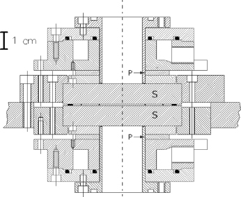
Figure 3. Conceptual design of the thermal-gradient cell. The sample is confined between two parallel sapphire windows (S). Annular Peltier devices in thermal contact with the sapphire windows pump heat through the sample.
Download figure:
Standard imageThe sample was confined within a cylindrical chamber of height h = 1.00 mm and diameter 25.0 mm. The chamber was bounded by two parallel, 12 mm-thick sapphire windows (S) that were temperature controlled to better than ±0.01 K. The use of sapphire windows allowed the application of a uniform temperature difference by using annular Peltier devices, while permitting optical access to the sample in a direction parallel to the imposed gradient. The sample was illuminated with collimated light from a super-luminous LED (SLD) with a wavelength of 680 nm, coupled to a mono-mode optical fibre. Interference between the beam and the light scattered by the fluctuations resulted in a maximum variation of the order of 3% of the intensity in the images collected by a charge-coupled device (CCD) with 1024 × 1024 square pixels. The region of interest (ROI) comprised the central 512 × 512 portion. Differences of images were Fourier decomposed to determine the mean-squared amplitude of concentration fluctuations versus the scattering wavevector q. Further details of the apparatus can be found in [17]. The experimental cell was filled on Earth six months before the mission. Material compatibility tests performed in the preparatory phases of the project showed no appreciable sign of ageing over the above-mentioned period.
Measurements were performed on board the FOTON M3 recoverable satellite. FOTON is an unmanned spacecraft that achieves very low overall g-jitter as compared to manned platforms (e.g. Shuttle flights, or the International Space Station (ISS)). Throughout the entire mission, the quasi-steady gravity level was between 10−5 and 10−6g [20]. More recent experiments performed on board the ISS showed that g-jitter levels typical of a manned spacecraft still do not produce any noticeable perturbation in mass diffusion processes [21]. To corroborate further, we have calculated the structure factor S(q) for non-equilibrium density fluctuation in a single-component fluid (see par. 5) at steady gravity levels other than 0 and 1g. For a sustained 10−4g acceleration, S(q) differs from that for g = 0 by 1.5%. For a sustained acceleration of 10−5g, the difference is 0.15%. The maximum fractional difference occurs very near the crossover wavevector of 10 cm−1.
A measurement cycle started with an equilibration period at a uniform temperature of 30.0 °C for 260 min. At the end of this phase a set of 539 reference images was acquired to characterize the optical background in the absence of an imposed temperature difference as well as the camera noise. The equilibration phase was followed by the rapid imposition of a temperature difference across the sample, which started the diffusion process. The temperature differences utilized were 4.35, 8.70 and 17.40 K. The instrumental time required for the formation of a linear temperature profile was about 100 s, while the time required to create a steady-state concentration profile (τ0 = h2/(π2Dc)) was about 500 s; here Dc = 1.97 × 10⁻⁶ cm2 s−1 is the mass diffusion coefficient of the polymer in toluene.
Once the temperature difference was applied to the sample, non-equilibrium concentration fluctuations began to develop. Figure 4 shows a comparison between ground-based and flight images. Shadowgraph images were taken simultaneously both on the ground and in flight with the polymer solution and an applied temperature difference of 17.40 K. Images were taken 0, 500, 1000 and 2000 s (left to right) after the imposition of the temperature difference. The side length of each image corresponds to 5 mm. Shades of grey map the deviation of the intensity from the time-averaged intensity.
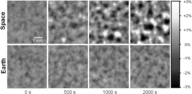
Figure 4. Shadowgraph images of non-equilibrium fluctuations in microgravity (top) and on Earth (bottom). The sample is a 1.00 mm thick solution of polystyrene in toluene. Images were taken 0, 500, 1000, and 2000 s (left to right) after the imposition of a 17.40 K temperature difference at t = 0. The side of each image corresponds to 5 mm. The shades of grey map the deviation of the intensity of shadowgraph images relative to the average intensity.
Download figure:
Standard imageThe figure shows that in a gravity-free environment, fluctuations are greatly increased in amplitude and spatial range. Images were acquired at a constant frame rate of 0.1 Hz while the gradient was held constant for 42 h. Estimates of the mean-squared amplitude of the fluctuations at various q were obtained by taking the azimuthal average of the two-dimensional power spectrum of image differences.
To isolate the signal from the concentration fluctuations from that due to non-equilibrium temperature fluctuations, as well as from other sources of noise (e.g. electronic noise from the CCD sensor), a dynamical analysis was performed (see [22] for details). The power spectrum was eventually divided by the instrumental transfer function T(q) to compensate for the oscillations of the shadowgraph transfer function.
The static structure factor of non-equilibrium concentration fluctuations S(q) obtained for temperature differences of 4.35, 8.70 and 17.40 K are shown in the top part of figure 5. The curves show the asymptotic power law behaviour S(q) ∝ q−4 for large values of q, while tending to saturate at low q due to the finite thickness of the sample.
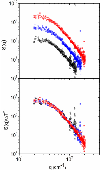
Figure 5. Top: experimental results obtained in microgravity in the presence of temperature differences of 4.35 K (black triangles), 8.70 K (blue squares) and 17.40 K (red circles). Bottom: experimental results divided by |ΔT|2. The scattering of points above 10 cm−1 is due to the normalization of the rapidly oscillating transfer function T(q).
Download figure:
Standard imageFrom the actual values of the fractional intensity fluctuations (see the grey scale in figure 4) one can derive an absolute estimate for the root-mean-square amplitude of the phase fluctuations generated by the non-equilibrium concentration fluctuations. This phase difference is of the order of 10−2 rad. The proportionality of the amplitude of non-equilibrium concentration fluctuations to |∇T|2 is confirmed in the bottom part of figure 5.
Experimental data from the space mission were compared with existing numerical predictions and with experimental data acquired on the ground during the space experiment. In the absence of gravity, and with the radius of gyration of the polymer chains much larger than the size of solvent molecules, a theoretical model [24, 25] based on a single-mode Galerkin approximation predicts that the mean-squared amplitude of fluctuations should scale onto a universal curve independent of mixture properties or applied concentration. Figure 6 shows the comparison of the experimental data with the predicted shape of S(q). This result provides a straightforward confirmation of the scale invariance of the fluctuations up to wavelengths comparable to the sample thickness, and an increase of the mean-squared amplitude of the fluctuations by more than two orders of magnitude at small wavevectors, as compared to theoretical predictions for the amplitude of the fluctuations on Earth (dashed lines). Above a length scale comparable to the sample thickness, the results confirm that the scale invariance of the fluctuations is broken by the finite size of the container, as predicted by theory [24] and by two-dimensional simulations [26]. Quite interestingly, recent simulations have shown that the presence of non-equilibrium concentration fluctuations affects the mass transfer during a diffusion process [27, 28].

Figure 6. Comparison of the experimental results for non-equilibrium concentration fluctuations with the theoretical predictions. The solid line is the theoretical prediction for microgravity. The dashed lines are the theoretical predictions for fluctuations on Earth. Because each data set has been scaled by its own high-q limit, this comparison is not sensitive to the actual amplitude of the fluctuations, but does serve to compare the predicted and measure shapes for S(q).
Download figure:
Standard image5. Non-equilibrium density fluctuations
The shadowgraph apparatus for the single-component fluid used a larger fluid cell, 75.0 mm in diameter and 3.00 mm thick, requiring significant changes to the optical configuration. The cold side of the fluid cell was silicon with a reflective multi-layer dielectric coating instead of a transparent element, and a beam splitter was inserted into the optical path between the SLD source and the lens. Thus the light passed through the cell twice, and was then directed to the sensor by the beam splitter. The high thermal conductivity of silicon relative to other typical optical materials (i.e. quartz, sapphire) improved lateral thermal uniformity and allowed heat to be easily removed by four thermoelectric elements in contact with the back surface of the silicon mirror. The collimating lens served to determine the magnification and effective viewing distance (z = 310 cm). The reduced physical volume of the folded optical path resulted in a very compact geometry suitable for flight experiments and also doubled the phase perturbations experienced by the light, resulting in a factor of four enhancement in S(q).
It is worth commenting on the remarkable sensitivity of the instrument and the quality of the data. The robust nature of the heterodyne technique along with quite practical data reduction methods allows one to perform measurements of small signals with high dynamic range and in wavevector ranges inaccessible to normal scattering techniques. For example, a wavevector of 20 cm−1, corresponding to a physical fluctuation of wavelength 3 mm and an astonishingly small scattering angle less than 0.01° is easily accessible with the shadowgraph technique. Ordinarily such small scattering angles are inaccessible due to stray elastically scattered light that overwhelms the true scattering, however, with the shadowgraph method such stray light must be able to affect the transmitted beam intensity to be significant, and thus the method is very insensitive to stray light.
We show in figure 7 a typical result for the azimuthal average of the two-dimensional power spectrum of CS2 density fluctuations on ground versus the dimensionless wavevector qL, for a small applied temperature gradient of 7.9 K cm−1. Here L is the sample thickness of 3.00 mm. The oscillatory behaviour associated with the transfer function, T(q), is clearly present. For quantitative comparison with theoretical predictions, the instrumental response was measured separately using a suspension of 2 μm diameter polystyrene latex spheres in isopropyl alcohol. Both the ground-based data and the transfer function measurements were made using the flight apparatus, after the flight. Over the wavevector range of interest, the spheres scatter uniformly, and are thus an ideal calibration standard. During calibration, the apparatus was tilted 90° and a small gradient was applied such that convection randomized the positions of the spheres between images. Data taken under the same conditions were used to measure the small background associated with temperature fluctuations in the alcohol. Spectral analysis of statistically independent images yields, after background subtraction, the transfer function [29].
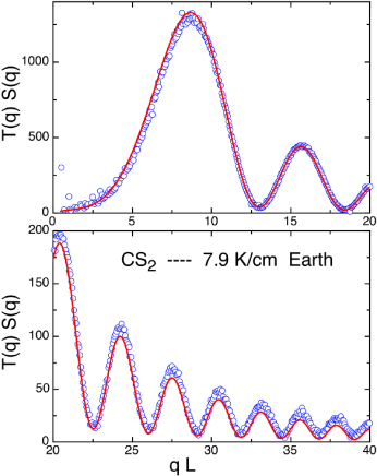
Figure 7. T(q)S(q) in absolute, dimensionless units for fluctuations on Earth in a 3.00 mm thick layer of CS2 heated from above versus the dimensionless wavevector qL with an applied gradient of 7.9 K cm−1. For the sake of clarity, the wavevector range 0–40 has been divided into two panels with different y-axis scale. Data appear as open circles. Theory is shown as solid line.
Download figure:
Standard imageThe data are shown as open circles, and the theoretical prediction [30] for S(q) multiplied by the measured transfer function T(q) is shown as the solid line. No parameters, including the amplitude, have been adjusted; thus, the theoretical prediction does a remarkable job of describing the data in both absolute amplitude and wavevector dependence.
The measured and theoretical structure factor S(q) for ground- and flight-based data are shown together in figure 8, for several applied gradients. This was accomplished by dividing the experimental result S(q)T(q) by the measured transfer function T(q). Considering the small numbers near the minima of T(q), the results are respectable. Both on Earth and in microgravity the data show reasonable agreement with theoretical predictions over a wide range of length scales and temperature gradients. Fitting the Earth-based data to the theory using a single adjustable overall scale factor gives values between 0.94 and 1.07 over an applied gradient range of 4.5–101 K cm−1. The analysis of the flight data was complicated by noise from an unknown source and an unexpected, slowly evolving structure in the raw images. However, it was found that S(q)T(q) could be extracted by fitting the theory to the time-domain spectral power, a process we will discuss further below. The peak in S(q) near qL = π, corresponds to fluctuations having a wavelength twice the thickness of the cell. Thus, without the presence of gravity, the finite size clearly limits the amplitude of the fluctuations.

Figure 8. Dimensionless structure factor obtained by dividing the raw data by the q-dependent transfer function T(q), versus the dimensionless wavevector qL, where L = 3.00 mm is the sample thickness. Applied gradients of 17.9K cm−1,34.5 K cm−1 and 101 K cm−1 are shown as blue squares, green triangles, and red circles, respectively. The upper curves show the data obtained during flight and the lower curves show data obtained on Earth after the mission. The solid lines are the theoretical predictions [30] without any adjustable parameters.
Download figure:
Standard imageIn addition to being used to determine the mean-squared amplitude of fluctuations, much as would be done using static light scattering, the shadowgraph technique can also be used to measure the temporal power spectrum of the fluctuations, S(q,ω). This provides the same information as would normally be obtained using dynamic light scattering. In the absence of gravity, the fluctuations decay diffusively, but for sufficiently low wavevector this is not the case when gravity is present. Instead, parcels of fluid that have been displaced may show oscillatory behaviour, which is revealed by S(q,ω), which develops a well-defined spectral mode at finite frequency.
An example is shown in figure 9 for an applied gradient of 51.2 K cm−1 at qL = 6.15. Interestingly, the theoretical model [31] matches the time-domain spectral power for ω > 8 s−1, but the theory overestimates the peak height and underestimates the contribution near ω = 0, with the integral being close to the theoretical value predicted for S(q).
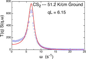
Figure 9. Time-domain power spectrum T(q)S(q,ω) at qL = 6.15 for CS2, measured with an applied gradient of 51.2 K cm−1 on Earth. Data appear as open circles, and theory [31] is shown as a solid line.
Download figure:
Standard imageConversely, fluctuations in microgravity retain their diffusive nature while growing immensely in amplitude. The data showed some anomalous, slowly evolving behaviour visible in the images and S(q,ω). Good agreement with the time-domain theory was observed for the data with ω greater than 0.2 s−1 (0.03 Hz), as shown for the applied gradient of 51.2 K cm−1 at qL = 6.15 appearing in figure 10.

Figure 10. Time-domain power spectrum T(q)S(q,ω) at qL = 6.15 for CS2 measured with an applied gradient of 51.2 K cm−1 in microgravity. Data (theory) appear as open circles, and the theory is shown as a solid line.
Download figure:
Standard imageBy fitting to the time-domain power spectra measured in microgravity and integrating the result to generate results for T(q)S(q), the shadowgraph method can produce reasonable results even for an applied gradient as small as 7.9 K cm−1, as shown in figure 11. For any system where an accurate time-domain model is available, and fluctuations occur over sufficiently long timescales, quantitative shadowgraphy should be capable of measuring even weaker fluctuations using this approach.
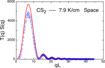
Figure 11. T(q)S(q) in absolute, dimensionless units for fluctuations in microgravity in a 3.00 mm thick layer of CS2 versus the dimensionless wavevector qL with an applied stabilizing gradient of 7.9 K cm−1. Data (theory) appear as open circles and the theory is shown as a solid line.
Download figure:
Standard imageIn conclusion, we have presented measurements of temperature and concentration fluctuations in reduced-gravity conditions. Results show a substantial increase of the amplitude of fluctuations at low wavevectors. Ultimately, fluctuations that are microscopic on Earth are limited in space by the dimension of the container in the direction parallel to the thermal gradient (1 mm for the mixture sample and 3 mm for the CS2 sample). Because the decay of fluctuations is governed by diffusion over the entire range of wavevectors in the absence of gravity, the lifetime of fluctuations at low wavevector is substantially higher than on ground. This may have profound implications for physics and biology experiments carried out on the International Space Station and other microgravity platforms. It is in fact commonly believed that the elimination of buoyancy driven convection guarantees the right environment for experiments that involve solidification or growth processes. Fluctuations are often disregarded, being of negligible size and lifetime on ground. The results here presented suggest that the enhancement of size and lifetime of density fluctuations should be also considered besides other factors (like g-jitter) that are usually taken into account when planning physics experiments in space.