

Abstract
Aiming at solving the existing sharp problems by using singular value decomposition (SVD) in the fault diagnosis of rolling bearings, such as the determination of the delay step k for creating the Hankel matrix and selection of effective singular values, the present study proposes a novel adaptive SVD method for fault feature detection based on the correlation coefficient by analyzing the principles of the SVD method. This proposed method achieves not only the optimal determination of the delay step k by means of the absolute value  of the autocorrelation function sequence of the collected vibration signal, but also the adaptive selection of effective singular values using the index
  corresponding to useful component signals including weak fault information to detect weak fault signals for rolling bearings, especially weak impulse signals. The effectiveness of this method has been verified by contrastive results between the proposed method and traditional SVD, even using the wavelet-based method through simulated experiments. Finally, the proposed method has been applied to fault diagnosis for a deep-groove ball bearing in which a single point fault located on either the inner or outer race of rolling bearings is obtained successfully. Therefore, it can be stated that the proposed method is of great practical value in engineering applications.
Export citation and abstract BibTeX RIS

Content from this work may be used under the terms of the Creative Commons Attribution 3.0 licence. Any further distribution of this work must maintain attribution to the author(s) and the title of the work, journal citation and DOI.
1. Introduction
Rolling bearings are one of the most common classes of mechanical elements and play an important role in industrial applications. They generally operate in tough working environments and are easily subject to failures, which may cause machinery to break down and decrease machinery service performance such as manufacturing quality, operation safety, etc [1–3]. Therefore, increasing reliability with respect to possible faults has attracted considerable interest in mechanical fault diagnosis in recent years [4, 5]. Finding adaptively effective signal-processing techniques to analyze vibration signals and to detect fault features has become a key problem in mechanical fault diagnosis. Meanwhile, it is also a challenge to propose and apply effective signal-processing techniques for extracting the crucial fault information from the collected vibration signals.
Currrently, traditional signal-processing technologies, including time-domain and frequency-domain analysis, are applied in mechanical fault diagnosis, such as wavelet transform (WT) [6, 7], ensemble empirical mode decomposition (EEMD) [8], singular value decomposition (SVD) [9], etc. The essence of these signal processing techniques is restraining or eliminating noise. Among these signal-processing methods, however, SVD has exhibited a very good performance which is widely used to extract the fault features of rolling bearings in mechanical equipment, especially impulse features. Zhao et al [10] pointed out the similar mechanism of signal processing between SVD and WT, which is analyzed from the basis vector space angle and the characteristic of the Hankel matrix. Liu [11] presented a method of detecting abrupt information from the vibration signal, which uses SVD based on the Hankel matrix created by time series to extract early rub-impact faults between rotor and stator in rotating machinery. Kang Myeongsu et al [12] proposed SVD-based feature extraction method for fault classification of an induction motor, whose classification accuracy using a support vector machine (SVM) approach is very high. Subsequently, Brenner et al [13] investigated capability of extracting fault features from the flight data, and the comparisons between SVD and transformed-SVD detection results have been made. Although the above-mentioned literature has confirmed that the SVD method is an efficient and reliable tool for automated on-line analysis and mechanical fault diagnosis, there is very little literature to research the effect of different delay step k values for detection results and application of SVD in impulse signal detection. On the basis of analyzing the literature, two major problems restricting the application of SVD for impulse signal detection and mechanical fault diagnosis are summarized, especially in the field of rotating machinery. One is the determination of the delay step k for creating the Hankel matrix. A different delay step k can produce different reconstructed signals obtained by SVD. However, in nearly all of the research that we can see, the delay step k is subjectively fixed as a constant, generally 1, which not only loses generality but also does not consider the influence of different values of the delay step k on the reconstructed signal. According to the creation principle for the Hankel matrix, one can see that a smaller delay step can make the cross-correlation higher between two adjacent row vectors of Hankel matrix, causing information redundancy, whereas with larger k there is smaller information redundancy but many more data points are required for creating a Hankel matrix of the same dimension [14]. In addition, if the delay step is too small, then its Hankel matrix is a kind of ill-posed matrix [15], which can cause the reconstructed signal to be inaccurate due to the solution being approximate. Thus, it is necessary to research the effect of different delay steps for the reconstructed signal in order to propose a novel method of determining a proper delay step.
The other problem concerns how to select effective singular values to obtain the optimal reconstructed signal and detect fault features. Now for this problem, methods such as the difference spectrum of singular values (DSSV) [9, 16], median value of singular values, and mean value of singular values can be employed to select effective singular values for getting the reconstructed signal. But these indices merely consider the magnitudes of singular values in terms of individual or global magnitude, and take no consideration of the contribution rate of each singular value to the original signal. These selection methods can cause weak fault features corresponding to smaller singular values to be eliminated and removed; conversely, strong disturbance information corresponding to greater singular values will remain, eventually causing difficulties in detection of fault features from the reconstructed signal. Therefore, it is vital for extracting mechanical fault features from the reconstructed signal to select suitable singular values.
In view of the above-mentioned problems which are of serious concern, the present study investigates SVD technology for mechanical fault feature detection and proposes an adaptively novel SVD method based on the absolute value of the autocorrelation function sequence to determine the delay step k for creating a proper Hankel matrix. On the basis of a large number of experiments, an effective measurement index  is proposed; by means of the minimum delay step k when
  (where
  is an experimental value), this method can implement an effective determination of the optimal delay step k. Then, in order to make good the disadvantages of traditional selection methods, a difference spectrum algorithm based on a normalized correlation coefficient is proposed in the consideration of the contribution rate of every component signal or singular value for the original signal because there is a one-to-one relationship between component signals and singular values. Simulated experiments and engineering applications demonstrate that the proposed determination and selection method is effective in detecting weak impulse signals and fault features of rolling bearings.
The remaining part of this paper is organized as follows. Section 2 introduces the SVD algorithm and existing problems, and the signal decomposition principle of Hankel matrix-based SVD and the essence of component signals obtained by SVD are studied. Then the influence of the delay step k for the reconstructed signal and singular values distribution is illustrated through simulated fault experiments, and a form of adaptive determination method for the optimal delay step is proposed in section 3. In section 4 the correlation coefficient singular value decomposition (CCSVD) method of adaptively selecting effective singular values for getting the optimal reconstructed signal is proposed; this method can correctly detect impulse features and fault information that are submerged in strong ambient noise. In section 5 the fault features of the inner and outer races of rolling bearings are detected using the proposed CCSVD method. Finally the conclusions are given in section 6.
2. Principle analysis of SVD method
For a collected discrete signal ![$\vec{X}=\left[x(1),x(2),\ldots ,x(N)\right]$](https://content.cld.iop.org/journals/0957-0233/26/8/085014/revision1/mst514168ieqn006.gif) , the Hankel matrix can be created using this signal as follows:
, the Hankel matrix can be created using this signal as follows:
where  , spectifically
  , and k is a constant integer called the delay step which generally is 1; then
  .
.
The definition of singular value decomposition (SVD) [17–19] is as follows: for a matrix  , two orthogonal matrixes
 ![$\vec{U}=\left[{{\vec{u}}_{1}},{{\vec{u}}_{2}},\ldots ,{{\vec{u}}_{m}}\right]\in {{\vec{R}}^{m\times m}}$](https://content.cld.iop.org/journals/0957-0233/26/8/085014/revision1/mst514168ieqn011.gif) and
and ![$\vec{V}=\left[{{\vec{v}}_{1}},{{\vec{v}}_{2}},\ldots ,{{\vec{v}}_{n}}\right]\in {{\vec{R}}^{n\times n}}$](https://content.cld.iop.org/journals/0957-0233/26/8/085014/revision1/mst514168ieqn012.gif) are guaranteed to exist that satisfy the following equation:
are guaranteed to exist that satisfy the following equation:

where ![${\vec \Sigma}=\left[\text{diag}\left({{\sigma}_{1}},{{\sigma}_{2}},\ldots ,{{\sigma}_{q}}\right),\vec{O}\right]$](https://content.cld.iop.org/journals/0957-0233/26/8/085014/revision1/mst514168ieqn013.gif) or its transposition, determined by
or its transposition, determined by  or
or  ,
,  , while
  is the zero matrix,
  , and
, and  . These
  are the singular values of matrix
  .
.
In order to implement the decomposition of a signal using SVD, equation (2) should be converted into the form of column vectors  and
and  :
:

where  ,
,  ,
,  , and
, and  . Based on the SVD principle, the vectors
  are mutually orthonormal and they form an orthonormal basis of m-dimensional space; the vectors
  are also orthonormal to one another and they form the orthonormal basis of n-dimensional space [20, 21].
Let  , then
  also. Supposing that
  is the first row vector of
  , and
, and  are k column vectors in the last k columns of matrix
  , as shown in figure 1, according to the creation principle for the Hankel matrix; if
  and all the row vectors of matrix
  are linked together in a given form as exhibited in figure 2, then a SVD component signal
  can be obtained, which can be expressed as the vector form

where  is the jth row vector of matrix
  ,
,  , and
, and  :
:

Figure 1. The principle for forming the component signal  when the Hankel matrix is used.
Download figure:
Standard image High-resolution image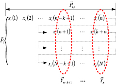
Figure 2. The initial and terminal segments of component signal  .
.
Download figure:
Standard image High-resolution imageAll the component signals formed by  make up one kind of decomposition for the original signal
  . To research what these component signals reflect in nature, first we might as well divide the component signal
  into two segments, as illustrated in figure 2, in which the initial segment is
  , is the first row vector of
  , while the terminal segment is the sequential connection of
  row vectors of matrix
  , where
  is formed by the last k column vectors of
  and the connection method is drawn by using the dotted line with arrows. It can be seen that if the delay step k is equal to 1, the terminal segment of component signal
  is the last column vector of matrix
  , highlighting a prevalent problem in which the effect of the delay step has been implicitly ignored. However, to extensively research the essence of the component signal, we will consider that k is not necessarily equal to 1; in this situation the terminal segment is a successive arrangement of the row vectors of matrix
  .
.
Suppose that the Hankel matrix  with delay step k created by the original signal is expressed by row vectors
  . As is known from the creation principle for
  , the first vector
  is the initial segment of the original signal and its projective coefficient on the basis vector
  of n-dimensional space can be computed from equation (2) as follows:

where  is the first element of basis vector
  .
.
 , which is the initial segment of component signal
  and also the first row vector of matrix
  , can also be calculated according to the definition of
  as below:

One can easily see that  is the product of basis vector
  and projective coefficient of
  on this basis vector, in which the projective coefficient
  decides the magnitude of
  , and vector
  determines the direction of
  . While
  is the initial segment of the original signal, so obviously
  is actually the projection of the initial segment of the original signal on the vector
  , which is the ith basis vector of n-dimensional space, and this relationship is illustrated in figure 3(a).

Figure 3. The essence of component signal  : (a) essence of the initial segment of
  ; (b) essence of the terminal segment of
  .
.
Download figure:
Standard image High-resolution imageSimilarly, supposing that the Hankel matrix  created by the original signal is described by the column vectors
  , as is known from the construction principle of
  , these column vectors
  are the terminal segment of the original signal, which is not a simple transposition of these column vectors
  but the sequential connection of row vectors of the arranged matrix by them and projective coefficients of column vectors
  on the basis vector
  of m-dimensional space can also be computed from equation (2):
where  is the nth element of basis vector
  .
.
The vectors  , which constitute the terminal segment of component signal
  and also the last k column vectors of matrix
  , can be computed according to the definition of
  as follows:
It can also be seen that  are the products of basis vectors
  and projective coefficients of
  on these basis vectors respectively, with the projective coefficients
  determining the magnitudes of
  , while the vectors
  determine the directions of
  .
.  are the terminal segment of original signal, so
  are actually the projections of the terminal segment of the original signal on the vector
  , which is the ith basis vector of m-dimensional space, and this relationship is illustrated in figure 3(b). So from the above analysis we can see that under different delay step values the nature of singular value decomposition based Hankel matrix is in fact to decompose the signal into m-dimensional and n-dimensional spaces.
In order to further analyze the characteristics of this kind of decomposition, assuming  is described by row vectors
  , while
  is expressed by row vectors
  . According to equation (3), it is clear that each row vector of
  equals the sum of corresponding row vectors in all
  , therefore we can obtain

The matrix  lies within
  , where
  . Supposing that the corresponding column vector in
  is
is  , where
  , we can also see that
  equals the sum of the corresponding column vectors
  in all
  . Obviously, their transposition can also meet this relationship, i.e.
Based on the creation principle for the Hankel matrix, the original signal  can be described as the vector form
  , where the operator 'sub' sequentially takes the column vectors of matrix
  , so the component signal
  can also be described as the vector form
  . Then the sum of all these component signals is

Based on equations (9) and (10), the right side of the above formula can be written as  , so
, so

Under different delay steps k, from equation (12) it can be seen that when the Hankel matrix is used, the component signals obtained by SVD can form a simple linear superposition for the original signal. This conclusion extends the range of the studies in [22–24], in which the delay step k is equal to 1. The advantage of this linear superposition is that the isolation of one component signal from original signal corresponds to simply subtracting this component from the original signal, and this subtraction computation will make the isolated component signal keep its phase the same as in the original signal; thus, there is no phase shift in the isolated component signal. Equation (12) is also the reconstruction formula for Hankel matrix-based SVD, and it is important that several effective component signals [25–27] can be simply added together to extract the feature information of the original signal.
3. Determination method of delay step k
To solve the above-mentioned problem, an effective method is proposed to create the proper Hankel matrix. For a collected discrete vibration signal ![$\vec{X}=\left[x(1),x(2),\ldots ,x(N)\right]$](https://content.cld.iop.org/journals/0957-0233/26/8/085014/revision1/mst514168ieqn125.gif) , the autocorrelation function sequence is calculated using equation (13):
, the autocorrelation function sequence is calculated using equation (13):
Here, we consider positive and negative correlations, so the absolute value of the autocorrelation function sequence is identified as index  , which can reflect the cross-correlation between two adjacent row vectors of Hankel matrix. The greater the value of
  , the greater the correlation between two adjacent row vectors of the Hankel matrix. Through a number of experiments of different impulse signals and signal-to-noise ratios (SNRs), impulse signal amplitudes generated by one impulse fault are different, and the SNR in the simulated fault signal is different. We find that the delay step k is satisfactory when the index
  is initially less than 0.1, which is an experimental value. The value weakens the correlation between two adjacent row vectors to reduce information redundancy and eliminate the problem of an ill-posed matrix [15]. Likewise, suitable data length for creating the Hankel matrix is required. In addition, the SNR is also relatively higher. This is also a compromise between information redundancy and data length required.
In order to verify the performance of proposed determination method, an impulse signal in [28] is employed to simulate bearing fault impulse, shown in figure 4(a). Gaussian white noise with SNR −9.6461 dB is added into the periodic impulse signal to obtain the simulated fault signal of rolling bearings, which can be shown in figure 4(b) where the sampling frequency is 20 000 Hz. The periodic impulse signal submerged in the surrounding noise can effectively simulate the tough operating environment of mechanical equipments. Thus, it has practical significance that the simulated fault signal can be employed to research the effect of delay step k for detecting fault features by using SVD method.
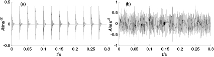
Figure 4. The bearing fault signal: (a) simulated impulse signal; (b) simulated fault signal.
Download figure:
Standard image High-resolution imageTo research the effect of different delay steps for detection capability, we consider situations in which k is 1, 2, and 3 respectively. Assuming that the simulated fault signal is long enough, a Hankel matrix with m = 1700 rows and n = 20 columns [10] is created using this simulated fault signal; 20 singular values can be obtained by the SVD method, as shown in figure 5. One can easily see that the first two singular values are relatively larger than any others, and there is a very large leap between the second and third singular value no matter what k is. This tells us that the characteristics of the impulse signal can be hidden in the first two singular values. With the gradual increase of k, however, the first two singular values start to rise slowly, and any other values may also descend slowly, with the gap between them becoming smaller and making the curve smoother. These changes can eliminate false peaks and make true peaks higher in the DSSV. Traditionally speaking, the larger singular values can contain much more useful fault features, which should be effective ones [16] corresponding to the component signals having more fault information and less noise. Thus the above phenomena indicate that the effective singular values will be enhanced and the ineffective ones will be weakened with the increase of k. According to the DSSV, the first two singular values should be selected to reconstruct the original signal; the reconstructed signals with different delay steps are exhibited in figure 6. It is clear that the impulse signal can be extracted effectively and correctly in three figures, whose periods of 0.025 s can meet the given period in figure 4(a). Likewise, the surrounding noise is eliminated to a large extent, and by comparing the three figures one can easily see that the detection result at k = 3 has higher amplitude than the one at k = 1 and less noise than the one at k = 2. Relatively speaking, the detection performance at k = 3 is more satisfactory. In addition, the SNR between the three reconstructed signals and the simulated fault signal and data length required can be calculated respectively, as shown in table 1. With the increase of k, we can see that, first, the SNR may start to rise rapidly and then decline gradually, and second, the data length required for creating the Hankel matrix should be  , in which the larger k can cause a longer data length required for creating a Hankel matrix of the same dimension. Figure 6 and table 1 tell us that the optimal delay step should be 3 rather than 1 in terms of the best compromise.
Table 1. Data length required and SNR for different k.
| k (delay step) | N (data length required) | SNR (signal-to-noise ratio) |
|---|---|---|
| 1 | 1719 | − 5.2873 |
| 2 | 3418 | − 4.0538 |
| 3 | 5117 | − 1.7861 |
| 4 | 6876 | − 2.1672 |

Figure 5. Singular values of simulated fault signals for different k.
Download figure:
Standard image High-resolution image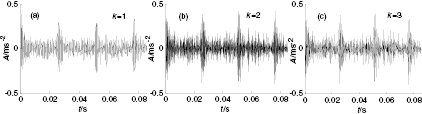
Figure 6. Reconstructed signal obtained by SVD for different k.
Download figure:
Standard image High-resolution imageSummarizing and analyzing the above three cases, first, we can clearly see that the energy of the original signal will be mainly concentrated in the first few component signals, which correspond to the first few largest singular values. Therefore, the first few component signals reflect the main skeleton of the original signal and achieve a similar effect to that of the approximation signal in wavelet transform. Meanwhile, detail features with low energy in the original signal will be isolated to the other component signals, which correspond to much smaller singular values. Second, there is no phase shift in component signals due to different delay steps k. In other words, the component signals obtained by the matrix-based SVD method have no phase shift no matter what k is. Finally, the processing and denoising effects of the reconstructed signal for different k are different.
The index  of the simulated fault signal is calculated using equation (13), as shown in figure 7. With the increase of k, we can see that the index
  initially declines rapidly, then fluctuates slowly as the wave peaks appear. It is obvious that the minimum of k is 3 under the condition
  , in other words, in which k is the x-axis value of the first left-hand point (under black dotted line). The value of k obtained by using the proposed determination method can meet the analysis results simulated above, in which the SNR between reconstructed signal and simulated fault signal is more satisfactory and the data length required is suitable. In essence, however, the determination method not only weakens the correlation between two adjacent row vectors of the Hankel matrix to reduce information redundancy and to eliminate the problem of an ill-posed matrix, but also allows a reasonable data length for creating the Hankel matrix. It is also an effective compromise between information redundancy and required data length.

Figure 7. Index  of the simulated fault signal.
Download figure:
Standard image High-resolution image4. Selection method of effective singular values
Up to now, no fixed selection method of effective singular values to reconstruct the original signal has been found. The existing methods such as DSSV, median value of singular values, and mean value of singular values merely consider the magnitude of singular values in terms of individual or global magnitude, and take no consideration of the contribution rate of each singular value for the original signal. The performance of these traditional selection methods can be determined by the magnitude of individual or global singular values and gaps between each other, revealing two shortcomings: first, the loss of important fault features or significant noise remaining in the reconstructed signal. If the SNR is very low, then singular values corresponding to noise will be enlarged, causing a higher threshold. Thus the important features included in relatively small singular values will be lost [27]. If the SNR is relatively high, then the mean and median values of the singular values can be lessened to make the threshold lower. Therefore, much more noise may remain in the reconstructed signal, for example the median value method and mean value method of singular values; and second, there is the false peak value problem. Sometimes when dealing with signals with strong trend [18], such as aircraft engine health signals, one may hardly choose the right singular values by using the DSSV method due to the strong trend resulting in the false peak. To solve the above-mentioned problems, the CCSVD method is proposed in this section to select the effective singular values for obtaining the reconstructed signal. Assume that the original signal X is decomposed by SVD, and we can obtain a series of component signals  , and calculate autocorrelation functions
  using equation (14) as follows:
Then these correlation coefficients  may be computed among the autocorrelation function
  and
and  , and be normalized using equation (15):
where N is the length of the original signal, and  is the normalized correlation coefficient of jth component signal. Likewise, the difference spectrum of the normalized correlation coefficient is defined as

where  . The principle of selecting effective singular values for obtaining the reconstructed signal by using the index
  is: if the maximum peak of
  happens at j = k, then the first k singular values should be selected to reconstruct the original signal. But if the maximum peak of
  happens at j = 1, then the first two singular values should be selected.
In order to test and verify the proposed selection method, the simulated fault signal in section 3 is employed figure 8 with SNR of −10 dB. One can see that the fault impulse features are completely submerged in the surrounding noise. The index  of the simulated fault signal can be calculated using the determination method proposed in section 3. We can obtain an optimal delay step k = 3 when
  is initially less than 0.1, so the Hankel matrix can be created with n = 20 columns and m = 1700 rows based on k = 3. Then we can obtain the first 4 component signals, shown in figure 9. It is found that the periodic impulse features are exhibited in the component signals
  and
and  , but cannot be seen in other component signals. In other words the Hankel matrix with k = 3 can concentrate a majority of fault energy in the first two component signals.
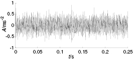
Figure 8. The simulated fault signal.
Download figure:
Standard image High-resolution image
Figure 9. The component signals  when k = 3.
Download figure:
Standard image High-resolution imageAdditionally, the values of  and
and  can also be computed according to equations (15) and (16), as shown in figure 10(b). It is obvious that the
  and
and  are larger than any others, and the difference spectrum
  can appear the highest spectrum peak at i = 2. According to the proposed CCSVD method, the first two singular values should be selected to obtain the reconstructed signal, which is exhibited in figure 11(c). Here we can see obviously periodic impulse features, and the surrounding noise has been weakened significantly. Compared with figures 8 and 11(c), we can also see that the impulse fault signal has been detected correctly by the CCSVD method, and there is also no phase shift in detection result. Although a small fraction of noise remains in the reconstructed signal (detection result), it is not very important for us to examine and extract the periodic impulse features. To make a comparison with the traditional SVD methods, figure 10(a) exhibits the singular values curve of the simulated fault signal, the median value and the mean lines for them, and the DSSV. The curve of singular values in figure 10(a) and the curve of the normalized correlation coefficient
  can be compared, and it can be seen that the first two greatest singular values in figure 10(a) correspond to the first two greater
  values, while the different singular values with amplitudes close to each other in figure 10(a) reflect different magnitudes of
  in figure 10(b). This tells us that different singular values of the same magnitudes have different contribution rates for the original signal. Thus, it is not correct when selecting effective singular values to consider merely the magnitudes of singular values. According to the selection principles of the median and mean value methods, we should choose these singular values above their lines to reconstruct the original signal, in which are first nine and first five singular values respectively. The reconstructed signals based on the median value and mean value methods can be obtained by SVD, shown in figures 11(a) and (b) respectively. Simultaneously, we can observe that the maximum peaks in the DSSV curve and of
  both occur at i = 2. According to the selection principles of the DSSV and CCSVD methods, we should choose first two singular values to reconstruct the original signal, and the reconstructed signals are shown in figure 11(c). To make a sufficient comparison, the detection result using a wavelet-based method is shown in figure 11(d), using the threshold function 'rigrsure', 3-layer decomposition, and wavelet base db3. By comparing the five detection results, it can be found that the detection result of the medianm value method in figure 11(a) has too much noise to observe the impulse features, while the mean value method in figure 11(b) can extract the impulse features but they are very weak. The wavelet-based method in figure 11(d) eliminates the excessive noise which causes the loss and damage of the impulse faults, and it is disadvantagous for us to observe the periodic impulse faults. However, the performances of CCSVD and DSSV methods are same and their detection results also relatively more satisfactory in all detection results. Thus, the above detection results prove that the proposed CCSVD method can properly select effective singular values to obtain the reconstructed signal, which only retains much fault information but also weakens the surrounding noise effectively. Of its nature, the proposed CCSVD method can select effective singular values based not on magnitudes of singular values themselves but on their contribution rates for the original signal, which can overcome the two above-mentioned shortcomings.
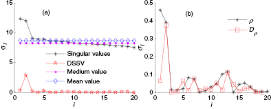
Figure 10. The selection indices: (a) the traditional selection methods; (b) proposed selection method.
Download figure:
Standard image High-resolution image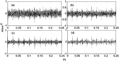
Figure 11. Comparison of five detection results: (a) median value method; (b) mean value method; (c) DSSV method and the proposed method; (d) wavelet-based method.
Download figure:
Standard image High-resolution imageThrough the above comparisons, one can see that the detection results of CCSVD and DSSV are the same for the impulse signal combined with Gaussian noise. To further prove the performance of the CCSVD method, suppose that there is a strong trend in the simulated fault signal [18], such as in an aircraft engine health signal. The strong trend can reflect and simulate the gradual increasing trend of a mechanical fault with time; therefore, a strong time (t) trend can be added into the fault signal simulated above. Using the determination method in section 3, we obtain the delay step as 2 and a Hankel matrix with 1700 rows and 20 columns can be created when k = 2. Then, the first 4 component signals can be obtained by SVD, which are exhibited in figure 12. It is clear that component signal  merely contains the prevailing trend of the fault signal, while the impulse fault information is hidden in
  and
and  . This tells us that the energy of the strong trend can be mainly concentrated in the first component signal, making the first singular value greater. Therefore, the strong trend can make the gap greater between the first two singular values as shown in figure 13(a), which can cause the appearance of false peaks in the DSSV. According to the selection principle of DSSV, if the maximum peak happens at i = 1, then we should choose the first two singular values to reconstruct the original signal; the reconstructed signal is shown in figure 14(a). Meanwhile, the detection result subtracted the component signal
  which includes the strong trend exhibited in figure 14(b). According to the selection principle of CCSVD, from figure 13(b) one can see that the maximum peak of
  happens at i = 3 and the false peak from the DSSV method can be eliminated and avoided. Thus, we should choose the first three singular values to get the reconstructed signal, as shown in figure 14(c) and the reconstructed signal with the strong trend
  subtracted can be exhibited in figure 14(d). By comparing the detection results, it is clear that the proposed method can correctly locate the peak and select effective singular values to reconstruct the original signal. In addition, the proposed method has overcome the shortcoming of the false peak from the DSSV method.

Figure 12. The component signals  when k = 2.
Download figure:
Standard image High-resolution image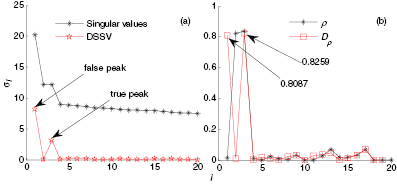
Figure 13. Two cases: (a) singular values and DSSV; (b) the contribution rate  and its difference spectrum
  .
.
Download figure:
Standard image High-resolution image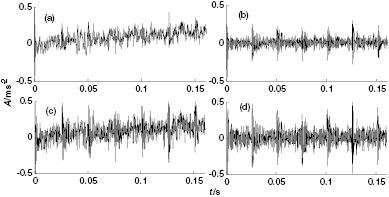
Figure 14. The detection results: (a) DSSV method; (b) strong trend subtracted using DSSV (a); (c) proposed CCSVD method; (d) strong trend subtracted using proposed method.
Download figure:
Standard image High-resolution imageThrough two experimental results for impulse signal without and with strong trend, the detection results have proved fully that the proposed method and DSSV have same performance in the processing of a signal without strong trend, better than any other traditional methods. Likewise, compared with the wavelet-based method, it is found that the SVD method has better impulse signal detection capability. Finally, a comparison has been made in impulse signal detection with strong trend, and the experimental results have testified that the proposed method can overcome the effect and disturbance of a false peak and correctly select effective singular values to get the optimal reconstructed signal.
5. Engineering applications
To verify the proposed diagnostic method, the test platform consists of a 2 hp motor, a torque transducer/encoder, a dynamometer, and control electronics. The test bearings which are 6205-2RS JEM SKF, deep-groove ball bearings, support the motor shaft. Single point faults were introduced to the test bearings using electrodischarge machining with fault diameters of 7 mm in both the inner and outer races. Vibration signal was collected using accelerometers, which were attached to the housing with magnetic bases. Digital data were collected at 12 000 samples per second. We consider the instability in the beginning of the data, so data points between 1000 and 7000 of the fault signals from the inner and outer races are selected to analyze for extracting the fault features, shown in figures 15 and 16, where figure 15(a) and 16(a) are the fault signal time-domain waveforms of the inner and outer race respectively, figure 15(b) and 16(b) their frequency spectra, and figure 15(c) and 16(c) their envelope spectra. According to fault characteristic frequency theory for rolling bearings, one can determine that the fault frequencies of the inner and outer race on the rolling bearing are 157.94 Hz and 104.56 Hz respectively, but it is very difficult to see the fault frequency from figures 15 and 16. The fault information is completely submerged in the strong surrounding noise.

Figure 15. Fault signal of inner race: (a) time-domain waveform; (b) frequency spectrum; (c) envelope spectrum.
Download figure:
Standard image High-resolution image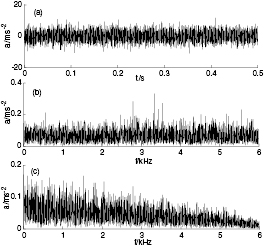
Figure 16. Fault signal of outer race: (a) time-domain waveform; (b) frequency spectrum; (c) envelope spectrum.
Download figure:
Standard image High-resolution imageIn order to detect the fault information, however, the proposed method in this paper is employed to process the fault signal of inner race and outer race of rolling bearings. The autocorrelation function sequence  can be calculated by using equation (13), where the minimum of delay step k are 1 (inner race) and 2 (outer race) respectively under the condition
  . Then, the Hankel matrix with n = 20 columns and m = 4000 rows is created by using equation (1) and the first five component signals
  can be obtained by SVD, as shown in figures 17 and 18. In figure 17, we can see the strong impulse features in component signals
  ,
,  , and
, and  , and the component signal
  has the modulated information to some extent. In figure 18, the component signals
  and
and  have the strong impulse features, and the component signal
  has a little modulated information. However, in the component signals
  and
and  there are also the weak impulse features, but the surrounding noise is also very strong, and relatively speaking the impulse features are very weak. Finally, the normalized correlation coefficients and difference spectra of the inner and outer race can be obtained according to equation (15) and (16) respectively, as shown in figures 19 and 20, and it is clear that the highest peak of
  happens at i = 5 and i = 3 respectively. Based on the proposed CCSVD method we should respectively select the first 5 and 3 singular values (inner race and outer race) to reconstruct the fault signal, as shown in figures 21 and 22, in which figure 21(a) and 22(a) show the time-domain waveforms of reconstructed inner and outer race fault signal, figure 21(b) and 22(b) their frequency spectra, and figure 21(c) and 22(c) their envelope spectra. One can see the weak impulse features for the inner race from figure 21(a), where the surrounding noise has been weakened effectively. At the same time, from its frequency spectrum in figure 21(b), we can observe that the frequency energy is concentrated in the frequency band between 2400 Hz and 4000 Hz. However, the frequency band of the noise is uniformly distributed in the white frequency band; in other words, the larger part of the noise is eliminated by the proposed CCSVD method. Finally the fault frequency is found to be 158.2 Hz (theoretical value is 157.94 Hz) from figure 21(c) and its amplitude is about 0.1, while the frequencies of noise and disturbance signal are concentrated in between 0 Hz and 1500 Hz, and their amplitudes are lower than 0.05. Compared with figures 15 and 21, we can see that the fault features are detected accurately and the surrounding noise is weakened effectively. Likewise, from the detection results of the outer race we can also see that the frequencies in figure 22(b) are concentrated in the frequency band between 3000 Hz and 4000 Hz and the frequencies in the other frequency bands are very weak. Comparing the envelope spectra in figure 16(c) and 22(c), it is clear that fault frequency of the outer race is 108.4 Hz (theoretical value is 104.56 Hz) and its amplitude is about 0.22. Additionally, it can be seen clearly that the double frequency is 213.9 Hz (theoretical value is 209.12 Hz). Therefore, the proposed method in this study has a better processing capability for weak impulse signal and a specific practical value in engineering applications.
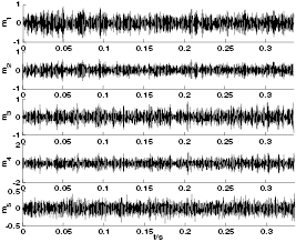
Figure 17. Component signals  of inner race by SVD where k = 1.
Download figure:
Standard image High-resolution image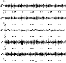
Figure 18. Component signals  of the outer race by SVD where k = 2.
Download figure:
Standard image High-resolution image
Figure 19. Normalized correlation coefficients and its difference spectrum for the inner race.
Download figure:
Standard image High-resolution image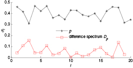
Figure 20. Normalized correlation coefficients and its difference spectrum for the outer race.
Download figure:
Standard image High-resolution image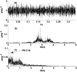
Figure 21. Reconstructed fault signal of the inner race: (a) time-domain waveform; (b) frequency spectrum; (c) envelope spectrum.
Download figure:
Standard image High-resolution image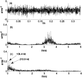
Figure 22. Reconstructed fault signal of the outer race: (a) time-domain waveform; (b) frequency spectrum; (c) envelope spectrum.
Download figure:
Standard image High-resolution image6. Conclusions
The signal decomposition principle of Hankel matrix-based SVD and the essence of component signals obtained by this method are studied. Meanwhile the mechanism of SVD method is analyzed from the basis vector space angle and characteristics of the Hankel matrix. By theoretical analysis and signal processing examples, the following conclusions can be drawn:
- 1.A signal can be decomposed into the linear sum of component signals by Hankel matrix-based SVD no matter what k is, and these component signals physically reflect the projections of original signal on the orthonormal bases of m-dimensional and n-dimensional spaces.
- 2.The energy of the original signal will be mainly concentrated on the first several component signals for the structure characteristics of the Hankel matrix in itself, which can be corresponding to the first several singular values.
- 3.With the change of delay step k the SNR is different between the reconstructed signal and the original signal, but there is no phase shift in all component signals. A Hankel matrix with n columns and m rows is created, in which n and m are fixed, and the data length required is
 which grows with increasing k. Thus the proposed determination method is an effective compromise between SNR, information redundancy, and data length required.
 - 4.The CCSVD method is proposed in section 4. This proposed method can eliminate the false peak in processing an impulse signal with strong trend and enhance the SNR in the reconstructed signal. Finally, it is applied to make fault diagnosis of rolling bearings. The experiments verify this proposed method is effective and accurate.

Acknowledgment
This research is supported by the Natural Science Foundation of Gansu province P.R China (1308RJZA273 and ZS021-A25-017-G) and the National Science Foundation of P.R China (50274003).