

Abstract
A parametric study of the factors contributing to peak-locking, a known bias error source in particle image velocimetry (PIV), is conducted using synthetic data that are processed with a state-of-the-art PIV algorithm. The investigated parameters include: particle image diameter, image interpolation techniques, the effect of asymmetric versus symmetric window deformation, number of passes and the interrogation window size. Some of these parameters are found to have a profound effect on the magnitude of the peak-locking error. The effects for specific PIV cameras are also studied experimentally using a precision turntable to generate a known rotating velocity field. Image time series recorded using this experiment show a linear range of pixel and sub-pixel shifts ranging from 0 to ±4 pixels. Deviations in the constant vorticity field (ωz) reveal how peak-locking can be affected systematically both by varying parameters of the detection system such as the focal distance and f-number, and also by varying the settings of the PIV analysis.
A new a priori technique for reducing the bias errors associated with peak-locking in PIV is introduced using an optical diffuser to avoid undersampled particle images during the recording of the raw images. This technique is evaluated against other a priori approaches using experimental data and is shown to perform favorably. Finally, a new a posteriori anti peak-locking filter (APLF) is developed and investigated, which shows promising results for both synthetic data and real measurements for very small particle image sizes.
Export citation and abstract BibTeX RIS

Original content from this work may be used under the terms of the Creative Commons Attribution 3.0 licence. Any further distribution of this work must maintain attribution to the author(s) and the title of the work, journal citation and DOI.
1. Introduction
Peak-locking (also referred to as pixel-locking or pixel-biasing) is a serious bias error source in PIV. It is the tendency for the measured location and displacement of a particle image to be biased towards integer values. Peak-locking will occur when the size of the diffraction-limited particle images on the sensor becomes too small, resulting in undersampled particle images [1]. Other forms of peak-locking, originating from poor correlation-peak interpolation or inadequate PIV methods, have previously been covered in great depth and are not discussed here [2, 3]. Particle images sizes should be between 2–4 pixels to keep the effects of peak-locking error to a minimal level [2]. Given the same lens and aperture, peak-locking effects are more pronounced for sensors with larger pixel sizes that are found in certain types of cameras suitable for PIV. In particular, high-speed cameras that use complementary metal–oxide semiconductor (CMOS) chips often have considerably larger pixels (10–20 µm) than CCD or sCMOS low-speed cameras (5–10 µm). These scientific-grade CMOS cameras are increasingly used in PIV as the desire for higher acquisition rates has increased. This demand has subsequently created a tendency towards even larger pixel sizes, as evidenced by the recent introduction of very high frame rate (20 kHz and greater) CMOS cameras with pixels as large as 28 µm. This newer evolution of very high-speed cameras has triggered a renewed interest in peak-locking and methods for mitigating the errors that it creates.
The errors associated with peak-locking adversely affect the estimation of turbulent statistics [4] and have therefore motivated a number of investigations. Numerous methods for reducing these effects a posteriori through data processing algorithms have been proposed. These methods include the use of a correlation mapping method [5], alternative sub-pixel displacement algorithms [6, 7], modifications to the particle displacement histogram [7, 8], spectral domain image shifting techniques [9], the use of simplified (1D) modeling and correction [10] and processing using phase correlations [11]. Methods have been suggested to prevent the undersampling form of peak-locking a priori by defocusing particle images or using large f-numbers have been discussed [2] but have not been studied extensively. In a recent study, the effect slightly defocusing particle images was found to be effective [12]. Despite these numerous methods for mitigating the effects of peak-locking, it is still often reported for experimental data, even from experienced PIV experimentalists (with a recent and notable example being case B from the 4th PIV challenge in 2014, [13]).
In this study, the peak-locking bias errors of a state-of-the-art PIV algorithm are examined using synthetic data to isolate the basic principles from effects associated with real cameras. The investigated parameters include: particle image diameter, image interpolation techniques, the effect of asymmetric versus symmetric window deformation and the interrogation window size. Some of these parameters are found to have a profound effect on the systematic and intensity of the bias error and these results are presented and discussed in detail.
Additionally, a simple experimental setup is proposed, allowing an easy and robust way of standardized peak-locking characterization for individual cameras: The camera is mounted above a precision turntable (running at a constant 33 rpm) that is equipped with a printed particle pattern of very small particle images. Focal length and camera distance are chosen such that the imaging is diffraction limited, comparable to most real PIV experiments. The rotating pattern results in a simple rotational velocity field, containing all sub-pixel shifts, from nearly zero pixel, up to a variable maximal shift (here about ±4 pixel). Since the constant rotation yields a constant vorticity throughout the measurement area, peak-locking errors can be visualized by displaying the z-component of vorticity (ωz). The effects of peak-locking can be quantified and minimized systematically both by varying parameters of the detection system such as the focal distance and f-number, and also by varying the settings of the PIV analysis.
A new and robust optical method is proposed to avoid peak-locking a priori: the usage of optical diffuser plates. These plates are typically used to spread the light intensity equally on Bayer pattern color sensors. They can be characterized as a birefringent diffuser with a spread of 10 µm and they are manufactured by LaVision. The diffuser plate is mounted in front of the sensor, introducing a slight defocusing effect on the image. Two of these plates may be staggered to increase the effect. The performance of this diffuser plate is compared in detail to other a priori methods, utilizing the aforementioned precision turntable experimental setup. When properly chosen, optical diffuser plates are shown to be as effective as defocusing [12]. Yet in contrast to defocusing, where optimal settings are difficult to find in practice, diffuser plates are more robust since their properties inherently prevent peak-locking reliably in a variety of challenging experimental conditions that are commonly found in PIV experiments. These include situations where the pixels can get back in focus by accident. An example of this situation is if the focal plane is not aligned exactly to the laser sheet (either through the use of a Scheimpflug adapter or focus-plane misalignment). Another example is where the focal plane is curved by optical distortions (measurement behind curved interfaces, such as cylinders or pipes). Also in certain measurement situations, it may not be possible or desirable to move the focal plane out of the illuminated region. An example can be found in volumetric measurements (tomographic PIV, 3D-PTV), where the diffuser will prevent the particles from being too sharp and small in the volume center. Finally, a new a posteriori anti peak-locking filter (APLF) is developed and investigated, which shows promising results for both synthetic data and real measurements.
2. Anti peak-locking methods
Methods aimed at reducing peak locking are investigated in this study, including a priori and a posteriori methods:
- 1.a priori methods:
- defocusing using a Canon remote focus ring
- recording using different lens apertures
- using no, 1× or 2× diffuser plates placed between lens and camera sensor
- 2.a posteriori methods:
- selecting optimal pixel interpolators (bilinear, spline) and interrogation schemes (asymmetric versus symmetric)
- application of the new APLF
The idea for the APLF is based on the observation that the bias error for bilinear symmetric interrogation scheme (see figure 1) is approximately point symmetric and periodic and has a wavelength of 2 pixels. Because of this property, for any point on the bias curve x, the bias at x − 0.5 pix has about the same intensity but the opposite direction of the bias at x + 0.5 pix. The APLF is implemented as a new image interpolator. When the interpolator is interrogated for a pixel at x, it returns the sum of the interpolated values at x − 0.5 pix and x + 0.5 pix, so that the bias errors are compensated. In practice the bias in x and y have to be compensated at the same time, so that the interpolator is implemented as:
where I(x,y) is the bilinear interpolated value at (sub-pixel) position (x,y). Imperfections of the filter in suppressing peak-locking completely result from the fact that the assumed conditions (point symmetric and periodic) do not hold exactly. This results in a remaining bias for the APLF.

Figure 1. Comparison of bias error versus particle shift for various interpolation schemes, showing the motivation for the APLF.
Download figure:
Standard image High-resolution image3. Synthetic test data
Synthetic PIV images are used to test the sensitivity of different PIV processing methods to particle image size. A random particle generator has been implemented that allows the creation of PIV images with particles of selectable diameter. The particle image diameter, dτ is estimated using the same method described in [2] and also recently described in [14], which shows that the width of the displacement-correlation peak, dD, is related to the particle image diameter by
As discussed in [2], the gradient parameter a can be neglected when dD is calculated by the autocorrelation function (ACF). The autocorrelation peak width here is calculated using the  width, is four times the standard deviation (4σ) of a Gaussian distribution. Solving for equation (2) yields the particle image diameter

It has been found to be necessary to compute the real integral over a pixel of the Gaussian particle function. Assigning e.g. only the value of the function at the center of the pixel leads to artifacts in the PIV analysis.
Particle images have been created with a size of 4096 × 4096 pixels. Particle density has been set to 0.05 particles per pixel, leading to 51 particles in a 32 × 32 window on average. This is even five times higher than the recommended number of 10 particles per window. Therefore, no problems are to be expected due to the low number of particles per interrogation window. Examples of the particle images are shown in figure 2. Note how each particle is represented only by a single pixel when creating particles with very small size, e.g. at the left of figure 2 with a particle image size of 0.4 pixels.

Figure 2. Synthetic PIV images with varying particle image sizes from 0.4 pixels (left) to 4.0 pixels (right), increasing by 0.4 pixels in 10 steps.
Download figure:
Standard image High-resolution imageA simple velocity field or particle shift field has been created to study the peak-locking effect. The particles are shifted between the first and the second image by a linear increasing distance in the x-direction (x-shift or u-component). The shift is zero pixels at the left hand side and is increasing linearly up to 6 pixels on the right hand side (see figure 3). The y-shift or u-component is zero in the complete field. Due to the slow change over 4096 pixels, the gradient in a 32 × 32 window is relatively small, below 0.05 pixels. This small linear gradient is not expected to cause any difficulties for the applied continuous window deformation PIV method. The height of the images with 4096 pixels is large enough, to get enough statistics from a single image: for 32 × 32 windows at 75% overlap, there are more than 500 interrogation windows in the y-direction (with constant flow conditions). For a 128 × 128 window, there are still 128 vectors.
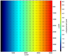
Figure 3. Displacement field for synthetic PIV data: x-displacement increases linear from 0 pixels (left) to 6 pixels (right). Not all vectors shown for clarity.
Download figure:
Standard image High-resolution image4. Experimental test data
Experiments with a high-speed camera (Phantom V711) have been conducted to study peak-locking with realistic imaging conditions. This camera has pixels that are 20 µm × 20 µm, which is mid-sized pixel for modern high-speed CMOS sensors (typically ranging from 16 to 28 µm). Designing a real PIV experiment where the flow field is sufficiently stable in time, while maintaining a fixed seeding density that contains a continuous range of particle shifts in a range between zero to six pixels, is very challenging. Instead, a turntable with a printed particle pattern is used to create a particle shift field that has a high temporal stability. The rotational speed is very precise and changes very little. Using the printed particle pattern ensures a constant seeding density.
Several recording sequences of 100 images each have been taken to study the effect of diffuser plates, defocusing and lens aperture on peak-locking. Details about the sequences are listed in table 1.
Table 1. Recording sequences and recording parameter.
| Diffuser plate | Lens aperture f# | Focus scan: positions | Images |
|---|---|---|---|
| No | 1.4 | 21 | 21 × 100 |
| No | 2.0 | 17 | 17 × 100 |
| No | 2.8 | 18 | 18 × 100 |
| No | 4.0 | 20 | 20 × 100 |
| No | 8.0 | 19 | 19 × 100 |
| No | 16 | 17 | 17 × 100 |
| No | 22.6 | 26 | 26 × 100 |
| 1 × | 1.4 | 21 | 21 × 100 |
| 1 × | 1.4–22.6 | 1 (in focus) | 7 × 100 |
| 1 × | 1.4–22.6 | 1 (slightly out of focus) | 7 × 100 |
| 2 × | 1.4 | 21 | 21 × 100 |
| 2 × | 1.4–22.6 | 1 (in focus) | 7 × 100 |
5. PIV analysis
Peak-locking is governed by characteristics of the imaging system, such as camera pixel size, magnification, focusing and aperture, but is also influenced strongly by implementation details of the PIV method that is applied. Parameters of potential influence are: the iteration type (single-pass versus multi-pass), the interpolation method for pixel interpolation (only for multi-pass), the type of window deformation that is applied (symmetric, asymmetric, deformed windows or simple window shift, discrete window shift or continuous shift or deformation) and the type of sub-pixel correlation peak interpolation. To concentrate on a manageable number of parameter and not to repeat results from the literature, here only the following parameter are varied and investigated:
- Correlation window size: 32 × 32 pixels for synthetic and experimental data and 128 × 128 pixels for synthetic data only
- Pixel interpolators for window deformation:
- 1.Single pass without interpolation (synthetic data only)
- 2.Bilinear (fast)
- 3.Spline interpolation of order 6 (slower but known to be more precise when particle images are large enough)
- 4.A new interpolator called APLF, designed to reduce peak-locking
- Symmetric versus asymmetric window (or image) deformation. In symmetric deformation, the velocity field at each location, V(x,y), is split in half and each half is applied equally to each image (of the image pair) at time t = 0 and time t = 0 + Δt. The asymmetric deformation is when the velocity field at each location, V(x,y), is applied to only the second image of the image pair at time t = 0 + Δt. See Scarano [15] for additional details.
To the authors' knowledge, the influence of the pixel interpolator and the influence of symmetric versus asymmetric window deformation on peak-locking and small particle image sizes (<1 pixel) has not yet been studied extensively. A notable exception is the work of Liao and Cowen [9], who did a detailed investigation of six different sub-pixel interpolators, including a bilinear particle image interpolator. The other parameters mentioned above are chosen to represent the current state of the art in PIV processing to the best knowledge of the authors:
- Gaussian shaped interrogation windows at 75% overlap
- Multi-pass processing (5 passes) with continuous interrogation window deformation and intermediate velocity field post processing (median filter and polynomial vector rectification).
All recordings and PIV analysis has been done using LaVision DaVis 8.3.0 software. The recording rate of the cameras was adjusted to 250 Hz to get a dynamic range of the pixel shift of ±3.5 pixels in x and y-directions (see figure 4).
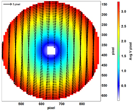
Figure 4. Particle shift turntable: the maximum shift at the outer border is about 3.5 pixels, giving a total dynamic range of 7 pixels (±3.5 pixels) in the x and y direction.
Download figure:
Standard image High-resolution image6. Results from synthetic test data
For the analysis of the synthetic data, the known true particle shift is subtracted. The remaining shift field contains random and bias errors, where the latter mostly depends on the sub particle shift, leading to a periodic bias error structure. Examples of the residual error are displayed in figure 5 for two different PIV parameter configurations. Particle size is increasing from 0.4 pixels (top) to 4.0 pixels (bottom). The residual clearly shows some random features (e.g. figure 5, top, left: small window size, small particles) but also quite systematic features, that are repeating periodically with the amount of sub-pixel shift in the (horizontal) x-direction. These systematic features are addressed as systematic bias error in the following. The strength of the bias error depends on the pixel interpolator and the particle image size. Usually the strength decreases with increasing particle image size, however there are exceptions from this which have to be discussed. Not only the strength, but also the wavelength of the systematic bias is different for different parameter settings: most settings show a periodicity with a wavelength of 1 pixel (in pixel-shift change). However, the bilinear pixel interpolator with symmetric window deformation exhibits a periodicity with two pixel of particle-shift change. To get a compact representation of the bias error, the u component of the error is averaged over all calculated vectors in the vertical (y) direction and displayed for all particle image sizes with respect to the particle shift (x-axis) in figures 6 and 7.
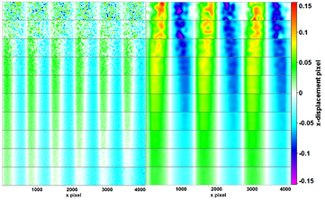
Figure 5. Deviation of u component from original particle shift. Left: 32 × 32 window size, single pass. Right: 128 × 128 window size, bilinear pixel interpolation, symmetric window deformation. Particle image size changes from 0.4 pixels (top) to 4.0 pixels (bottom) in steps of 0.4 pixels.
Download figure:
Standard image High-resolution image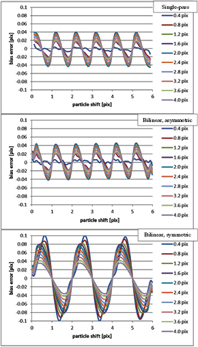
Figure 6. Bias error as a function of particle shift for different pixel interpolator and particle image sizes.
Download figure:
Standard image High-resolution image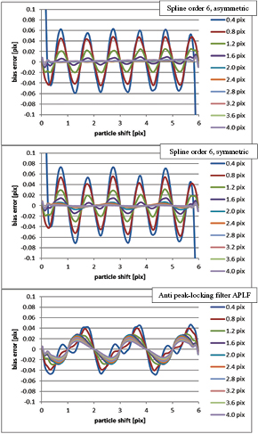
Figure 7. Bias error as a function of particle shift for different pixel interpolator and particle image sizes.
Download figure:
Standard image High-resolution imageThe most basic PIV procedure to study in terms of peak-locking is a single pass PIV processing (figure 6, top). Here no interpolation or window deformation is involved. Peak-locking will only depend on statistical properties of the particles and the sub-pixel correlation peak interpolator. Since there is no window deformation, there is also no differentiation between symmetric or asymmetric deformation. The maximum bias error observed in this configuration is about 0.04 pixels for 1.6 pixels and 2.0 pixel particle image size. Unexpectedly, the bias error is lower for smaller particle image sizes, reaching a minimum for particles with a size of 0.4 pixels. This is further discussed below in the context of figures 8 and 9. The same is true for the bilinear asymmetric interpolator (figure 5, center).
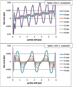
Figure 8. Bias error as a function of particle shift for different PIV interpolator and particle image sizes(magnified y-axis).
Download figure:
Standard image High-resolution image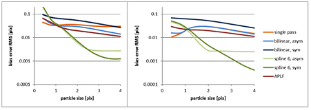
Figure 9. RMS of bias error as a function of particle image size for different interpolator. Left: window size 32 × 32, right: window size 128 × 128.
Download figure:
Standard image High-resolution imageKeeping the bilinear interpolator, but changing from asymmetric to symmetric window deformation changes the picture of the bias error completely (figure 6, bottom): The maximal bias error is much larger (above 0.1 pixels for smallest particles). The wavelength of the periodic bias error is doubled from 1 pixels shift-change to 2 pixels shift-change. Here the error is decreasing monotonically for larger particles but remains at a high level of up to 0.04 pixels even for the largest particle image diameters studied presently (4.0 pixels size). An interesting feature of the bias error for this interpolator is that it is nearly perfectly point symmetric, especially for small particle image sizes. This feature is exploited in the design of the APFL which has already been discussed.
Results from the spline order 6 interpolators are depicted in figure 7 (top and center) and in figure 8, where the bias error scale has been magnified by a factor of ten, allowing for a more precise visualization of very small bias errors for larger pixel sizes. The wavelength is again 1 pixel particle shift change for asymmetric and symmetric. The overall magnitude and structure is very similar between asymmetric and symmetric window deformations. A small difference is however, that for the symmetric case a slight period doubling is visible leading to alternating higher and lower peaks in the bias error curve (figure 7 center). Also, different from the other interpolators, the spline interpolator shows strong border effects for small particles for shifts of zero pixel (left border) and 6 pixels (right border) with increasingly high bias errors at the borders. This may result from the 'mirror' boundary conditions that are used in the implementation of the spline interpolator at the image borders, where pixels have to be 'guessed' when the interpolation kernel reaches beyond the image borders. The larger kernel (7 × 7 pixel) of the spline interpolator is effected much stronger by boundary effects than the small 2 × 2 kernel of the bilinear interpolators. For larger particles, the spline interpolators perform extremely well, reaching error as low as about 0.001 pixels (figure 8, bottom, purple curve) (apart from border effects, where the bias error is higher). That is why they are commonly used for higher order interpolation in the final passes. Interestingly the wavelength, only for the symmetric case, switches from 1 pixel to 2 pixels particle shift when increasing the particle image size from 1.2 pix (figure 7 center, green curve) to 2.0 pix (figure 8, cyan curve).
The effect of different interpolation schemes is shown in figure 9. In general, the spline 6 interpolator shows the lowest peak-locking error for particle image sizes of about 1.2 pixel or greater. In both the window sizes, the symmetric spline 6 had a lower error than the asymmetric as the diameter increased. For larger windows (128 × 128), the bilinear asymmetric show lower errors for smaller particle image sizes. This curious result is not found for smaller windows (32 × 32). The decreased RMS error for smaller particles is likely compensated by the overall higher noise level for the smaller interrogation windows. Also for large pixel image size (4.0 pix), the bias error is considerably larger for single pass than for bilinear asymmetric at a smaller window sizes (32 × 32), whereas for larger window sizes (128 × 128), the two curves are nominally identical across a wide range of particle image sizes. This is thought to be the result of how window deformation is carried out between image one and image two using an FFT correlator: as the shift to be detected becomes larger (up to six pixel), the overlapping part of the windows from image one and image 2 becomes less (32 pixels–6 pixels) and border effects from the cyclic nature of the FFT become more prominent. This is compensated in higher passes by the window deformation, leading again to a nearly 100% overlap in the final passes. The increasing effect of less window overlap in single pass can also be seen in figure 10, bottom left, where the bias error changes slightly from left to right as the overlap becomes smaller. The coincidences of the curves for single pass and bilinear asymmetric in figure 9, right, can also be interpreted as the multi-pass not being as effective for larger window sizes (128 × 128) with the bilinear asymmetric pixel interpolator, as the border effects of about 6 pixels play a much smaller role here. This is also visible by the similarity of the profiles in figure 6 between top and center.
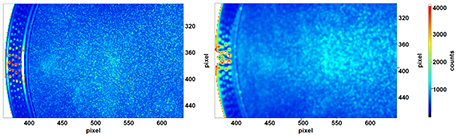
Figure 10. Particle pattern images from turntable recordings. Left: no diffuser, f# = 4, in focus, particle image size = 0.602 pix. Right: 2 × diffuser, f# = 1.4, out of focus, particle image size = 2.03 pix.
Download figure:
Standard image High-resolution imageThe plots in figures 7 and 8 give a good overview about the average performance of the interpolators. The results however are only valid for the average and do not give specific information about the performance for individual images. For example, two interpolators can have the same average bias error, while one of them shows only little variation about the average and the other shows strong variations. Strong variations imply that individual time steps may show substantially higher error values than the mean. Therefore, if not only the average is of importance, but also the individual, instantaneous results, the preferred method would be the one that is showing a smaller variation, assuming otherwise similar performance.
A more pronouced difference between single pass and bilinear asymmetric is observed in figure 11, showing the variance of the bias error for a given pixel size: single pass is also showing the smallest variance of the bias error for small particles. In contrast for larger particles, the variance is highest for single pass; in fact it is an order of magnitude higher than for the other interpolators and especially also much higher than bilinear asymmetric. This means that individual results (instantaneous velocity fields) will have much stronger deviations from the mean for single pass analysis compared to the other approaches for particles image sizes above 1.4 pixels. Below this size threshold, single pass shows suprisingly good performance for very small particles using synthetic data, e.g. it shows about 5 times less bias error at 32 × 32 windows compared to the spline 6 interpolators (figure 9, left). This effect was nevertheless regarded as having very little practical relevance, as single pass is known to show poor performance in the presence of gradients, which are common in real flow fields, but are not included in these synthetic data. For this reason, single pass has not been used in tests with the experimental data.
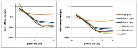
Figure 11. Variability (stdev) of bias error as a function of particle image size for different interpolators. Left: window size 32 × 32, right: window size 128 × 128.
Download figure:
Standard image High-resolution imageApart from the single pass, all of the interpolators show a similar variation in figure 11, which is strongly related to the actual average bias error: the lower the bias error, the smaller the variance. This also means, that in general the variance becomes smaller for larger particles. This will be shown to be different for experimental images, where the variance is going to increase after an optimal particle image size has been reached. Consequently the spline 6 interpolators show the smallest variance for larger particle image size, making this interpolator the most reliable one for individual time steps.
7. Results from experimental test data
It has been found that displaying the z-component of vorticity (ωz) is a straightforward and intuitive way to visualize and quantify the peak-locking effect of the constant rotation turntable flow investigated here (figure 12, top). Any deviation from a nominally constant vorticity value can be regarded as an error here. Systematic deviations from constant vorticity, which are attributed to peak-locking, are highlighted by averaging the detected particle shift fields from all 100 images. The numerical deviation from the constant vorticity is at the same time a quantitative measure for the peak-locking strength. This error is specified in the following as the percentage of the total constant vorticity (ωz) as 'vorticity error (%)', which can be thought of as a linear or at least monotonic measure of peak-locking strength. This error is found to cover a wide range from about 0.5% with optimal imaging conditions and optimal PIV processing settings, up to 42% for the smallest particle image size and PIV settings that are sensitive for peak-locking (e.g. figure 12, top right). In the following it is discussed how this error is affected by focal distance, lens aperture and diffuser plates.
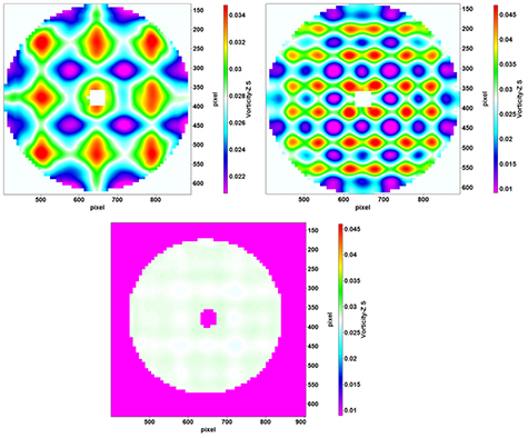
Figure 12. Vorticity contours: These should be constant values, but instead they show non-constant values due to peak-locking. Top left: bilinear symmetric, no diffuser, f# = 1.4, in focus; top right spline 6, symmetric, no diffuser, f# = 4.0, in focus. Deviation of measured vorticity from mean value defines the vorticity error, which is a measure of peak-locking. The checkerboard pattern corresponds directly to the wavelength of the bias error as detected with synthetic data. Bottom: nearly flat vorticity, low variation of measured vorticity showing much less peak-locking for 2 × diffuser, symmetric spline 6 interpolator, f# = 1.4, slightly out of focus (vorticity scale similar to top, right for comparison, for contrast reasons, missing vectors are pink here).
Download figure:
Standard image High-resolution image7.1. Focal distance
The effect of altering the focal distance is displayed in figure 13 using no diffuser plates for lens apertures of f# = 1.4 (top) and f# = 4.0 (bottom). The focal point is defined to be at the position of the largest error (focal distance = 0 m), the other values are plotted relative to this point using the relative focal distance as indicated by the remote focus control device, the Canon remote focus ring. The spline interpolators, both symmetric and asymmetric, show the strongest sensibility for changing focus: Depending on the focus settings they show both, the overall highest or overall lowest vorticity error. As the spline interpolators are most desirable because of their excellent performance at suitable particle image sizes, this highlights the tremendous importance of careful defocusing when working with cameras with large pixel sizes.
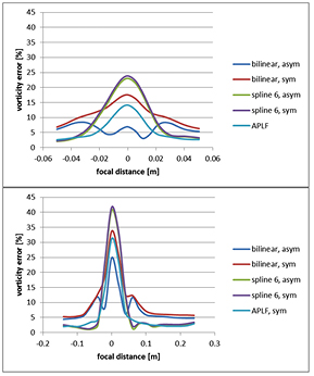
Figure 13. Effect of defocusing: No diffuser, Top: f# = 1.4, Bottom: f# = 4.0.
Download figure:
Standard image High-resolution imageThe focusing effect is much stronger at f# = 4.0 than for f# = 1.4, which at first hand seems to be counterintuitive as a smaller f# may be expected to give smaller diffraction limited particle spots on the camera sensor. But as has already been discussed by Overmars [12], the smallest f# does not create the smallest particle images due to imperfections of real lenses. In this example the smallest particle images seem to be produced at apertures of f# = 4.0 or f# = 8.0. This aperture is also known as favorable aperture in photography. This is good news for PIV, since it allows to use a smaller f# and in this way to gain more light and get less peak-locking at the same time.
Nevertheless, it should be mentioned, that the absolute smallest error, without using additional diffuser plates, is achieved exactly for the favorable aperture f# = 4 and optimal defocusing (figure 13, bottom, focal distance = −0.05 m or +0.07 m), although these optimal defocusing points may be hard to achieve in practice without performing explicit focal distance scans.
The bilinear asymmetric interpolator continues to show a non-monotonic behavior by expressing local minimal as the focal position is approached from left or right. The error values in the focal point, where the particle images are expected to be the smallest, are again the lowest among all interpolators, fitting well to the results from synthetic data (figure 9).
The APLF is the overall best performing symmetric interpolator in a wide range of focal distances. The spline 6 interpolator is better only in a narrow range of optimal defocusing for the spline 6 interpolator (as mentioned above).
The bilinear symmetric interpolator cannot be recommended in any case, as it is nowhere the best performing symmetric interpolator among all focal conditions.
7.2. Effect of aperture
The effect of changing the lens aperture alone (i.e. no diffuser plate is used) is illustrated in figure 14, top. The lens used for this study is a Canon EF 24 mm f/1.4 L USM. For all interpolators, the vorticity error changes very similar as the aperture f# is increased from 1.4 (left) to 22.6 (right). Showing border minima for f# = 1.4 and f# = 22.6, the error reaches local maxima for all interpolators at f# = 4.0 to 8.0. The difference between minima and maxima is about 20% in all cases (figure 14, top). The curves confirm the effect already discussed for f# = 1.4 and f# = 4.0 from figure 13: smallest particle images are not achieved for the smallest aperture f# = 1.4, but for the favorable apertures f# = 4.0 and 8.0 that result in the sharpest possible imaging. The aperture effects on the vorticity error are so strong, that the aperture must absolutely be taken into account. Fortunately, most PIV experiments are performed using the smallest f# available to gain as much light as possible, in this way avoiding the dangerous 'favorable' apertures ( f# = 4 and 8 in this case). The aperture effect alone is not strong enough to enlarge the particles so much that the spline 6 interpolator can show their strength. The spline 6 interpolators show the poorest performance in the whole aperture range, the interpolators already known to be good at small particle image sizes perform much better here (bilinear asymmetric and symmetric and the APLF. Additional defocusing and or diffuser plates would be necessary for the spline 6 interpolators for a better performance and lower vorticity errors.

Figure 14. Effect of aperture and diffuser: top: no diffuser, center: 1 × diffuser, bottom: 2 × diffuser, all in focus.
Download figure:
Standard image High-resolution image7.3. Effect of diffuser plates
The effect of including one or two diffuser plates between the lens and the camera sensor is shown in figure 14, top, center and bottom. As the number of diffuser plates is increasing from zero (top) to two (bottom), the observed vorticity error is decreased considerably and constantly, particularly for the apertures f# = 4 and 8 and for the spline 6 interpolators. The order of the interpolators performance now changes when using diffuser plates. The spline 6 interpolators perform relatively better by adding the plates. However, the APLF still performs better in all cases, confirming again, that spline 6 interpolators cannot be used satisfactory without further defocusing. Using 2 diffuser plates, the bilinear interpolators, asymmetric and symmetric, become less attractive, as they do not exhibit specifically low errors in this situation. The particle image size became already too large for this interpolators to take any advantage (figure 14, bottom).
7.4. Particle image size
Having studied the effects of defocusing, aperture and diffuser plates seperately, it would seem reasonable that there might be a common underlying principle that explains the performance of the interpolators and the peak-locking strength, as illustrated by the vorticity error. This common underlying principle could be affected by the alteration of the imaged particle image size by defocusing, changing the aperture, and adding diffuser plates. To show this principle more explicitly, an autocorrelation-based particle image size calculator is used, which allows the spatially resolved particle image size estimation from actual particle images. Before using this particle image size estimator for the interpretation of peak-locking effects, first a calibration curve is generated that shows the relation between measured particle image size and actual particle image size, based on the known particle image sizes from the synthetic images. Figure 15 shows that the particle image size is overestimated for small particles (left side of figure 15), where a particle image size of 1.2 pixels is measured when the actual particle image size was 0.4 pixels. This finding should be kept in mind when results are discussed later in terms of particle image size: small particles may actually be much smaller than measured. The measured particle image size becomes more accurate in absolute terms as the particles become bigger. Finally, at a particle image size of 4 pixels, the measured and the true particle image size coincide (right side of figure 15).
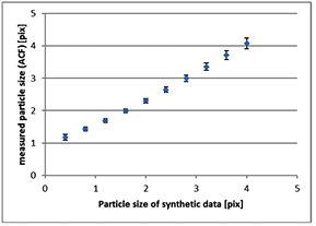
Figure 15. Particle size measured from synthetic data, using the ACF.
Download figure:
Standard image High-resolution imageTo check the consistency of the performance of the particle image size calculator for experimental data, the estimated particle image size is studied for changing focal distance, changing aperture and changing number of diffuser plates and the results are presented in figure 16, reproducing the conditions studied for figures 13 and 14. Changing the focal distance consistently leads to smaller estimated particle image sizes when approaching the focal point from the left or right. At the focal point, the particle image size shows minima for f# = 1.4 and 4. Especially for f# = 4, the minimum detected particle image size of about 1.2 pix corresponds to a real particle image size of about only 0.4 pixels, taking the calibration curve (figure 15) into account. This fits well to the estimated particle image size from diffraction theory, which is about 0.28 pixels for this case. This shows that the examination of synthetic particles of this size in the above sections has not been a purely academic exercise, but has an application in real world conditions.
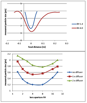
Figure 16. Particle image sizes from defocusing (top) and from different apertures (bottom).
Download figure:
Standard image High-resolution imageThe range of detected particle image sizes covers approximately the same range as the calibration curve (figure 15), ranging from 1.2 to 4.0 pix corresponding to real particle image sizes of 0.4 to 4.0 pixels. Measured particle image sizes are also consistent for changing apertures (figure 16, bottom), fitting exactly to the results obtained for the vorticity error: smallest particles are detected for the favorable apertures of f# = 4 and 8. Particle sizes are increasing for smaller and larger f#. So the distortions of real lenses are indeed proved to result in larger particle images for smaller f# = 1.4 as compared to f# = 4. The effect is similar in strength when compared to using large f#, e.g. f# = 22.6. This result shows that there is no need to use such large f# in planar PIV experiments and lose orders of magnitude of light intensity. Using two diffuser plates instead of no plate increases the measured particle image size from a minimum of 1.2 pixels to a new minimum of 1.8 pixels at f# = 4, corresponding to real particle image sizes of 0.4 and 2.0 pixels, respectively (figure 14).
All results shown in figure 16 confirm the idea to use the measured particle image size as the underlying variable to study the performance of different image interpolators, as will be done in the following.
7.5. Peak-locking and particle image size
The average particle image size has been calculated for each recording sequence of 100 images (table 1), averaged over all images in the sequence as well as spatially averaged over the whole image area (after applying a round mask including only the particle pattern). Detected particle image sizes reach from 1.2 pixels to 4.5 pixels corresponding to real particle image size of 0.4 pixels to 4.6 pixels (figure 15). 4.6 pixels particle image size seems to be the upper limit of particle image sizes that can be detected under the given experimental conditions. The autocorrelation method should be capable of detecting larger particles at least for synthetic data (this is to be studied in the future). However for this experiment there seems to be this upper bound of 2.3 pixels. This may be an artifact that is not only related to the real size of larger particles but more to the degrading imaging conditions that lead to large particles, like extreme defocusing, where the particle image shape starts to deviate from a spherical particle towards a blury particle image that can even include donut-like shapes, depending on the lens in use. So the measured value for larger particle image sizes should be considered to be approximate values, keeping in mind that the real particle image size may even be larger.
The performance of all interpolators in terms of particle image size and vorticity error is displayed in figure 17. The most consistent performance can be attributed to the APLF (figure 17, bottom left, dark red dots). Initially there is a steep monotonic decrease of the measured error with particle image size, which levels out for particles sizes of around 1 pixel. The error continues to decrease linearly at slower rate up to the maximal particle image sizes of 4.4 pixels. Compared to the other interpolators, the scattering of the error values at a particular particle image size is very small. Most of the scattering only occurs in a small region of particle image size between 1.5 pixels and 2.0 pixels. Figure 17, bottom, right again confirms, that APFL is the best-performing symmetric interpolator for particle image sizes up to 2.0 pixels.

Figure 17. Error in measured vorticity (RMS in %) from experimental data, with all recordings considered (table 1). Particle size is calculated using the ACF. Each data point represents an average from 100 velocity fields.
Download figure:
Standard image High-resolution imageBilinear interpolators, both asymmetric and symmetric show very similar results for particle image size above 1.2 pixels (figure 17, top left). While the symmetric interpolator is monotonic throughout the range of particle image sizes, the asymmetric interpolator shows a non-monotonic behavior, showing a local minimum at about 1.6 pixel particle image diameter. This is consistent with the findings in figures 9 and 12, where this interpolator is also showing an unusual non-monotonic behavior. For some reason, this interpolator exhibits less peak-locking for very small particle image sizes. The spreading of the vorticity error is at the same time relatively high, so that e.g. for a particle image size of 2.0 pixel, the measured vorticity error varies between 5% and 10%.
The asymmetric and symmetric spline 6 interpolators show very similar results in figure 17, top right. The highest (42%) and lowest errors (0.3%) are measured with these interpolators. There is a very smooth monotonic decrease of the measured vorticity error for increasing particle image sizes. There is also a large scattering of about 5% vorticity error, which makes it hard to predict the performance if one needs very small vorticity errors. Investigating the exact conditions under which the very best performance could be achieved (at the levels of 0.5% vorticity error) remains a topic for future studies.
The absolute minimal vorticity error of only 0.32% has been found for the asymmetric spline 6 interpolator, 2 × diffuser, f# = 1.4 and slightly defocusing. The smallest but one error of 0.66% for symmetric interpolators is again the spline 6 interpolator with the same conditions as above. Only slightly better with an error error of 0.64% is the symmetric spline 6 interpolator at f# = 2.8, slightly out of focus without diffuser plates. It should be noted that in contrast the largest errors can be as high as 42% in unfavorable conditions, that may easily occur in practice.
Figure 17 could suggest that the vorticity error gets ever smaller when using larger and larger particle images. This seems to be true for the average vorticity error. Figure 18 shows, however, that the variation of the errors gets considerably larger for larger particles, so that instantaneous results will scatter increasingly and will become more and more unreliable. Taking this into account, setting up the optical conditions (focus, aperture, diffuser plates) to get a measured particle image size of 2–3.5 pixels is strongly suggested to stay in an optimal range for minimal vorticity error, using the most precise spline 6 interpolators. This result agrees with the work of Cowen and Monismith [16], who examined the error associated with particle image diameter using Monte Carlo simuations.

Figure 18. Variation of vorticity error (stddev): different from synthetic data the variation is increasing again for larger particle image sizes. Possible reason: reduced image quality for out of focus images (more noise).
Download figure:
Standard image High-resolution image
8. Conclusion
State of the art PIV methods are able to calculate remarkably accurate particle shift fields when applied to images with particle image sizes of 2 pixels or larger. In particular, the symmetric spline-6 interpolator can achieve an accuracy of about 0.001 pixels with a 32 × 32 window when analyzing synthetic data. The same method suffers from errors of 0.1 pixels and larger if the particle image size is as small as 0.4 pixels, which is more than a hundred times larger than for optimal conditions. Moreover, this error is a systematic (or bias) error, which is not canceled out by averaging. As seen in figure 12, this error becomes very noticeable (averaging 100 images in this case).
The use of small f-numbers, which is a standard practice in PIV to get the maximum light from the expensive light sources, is already a good way to avoid the worst effects of peak-locking. Working at the most favorable f# (for photography at least), which was f# = 4.0 in this setup, results in 2 × higher vorticity errors (about 45%) than using the smaller f-number of 1.4 (25% error), which also gives considerably more light in a PIV experiment. Larger f-numbers than f# = 4.0 increase again the particle image size and reduce the peak locking errors. High-speed cameras with larger pixel sizes (more than 20 µm) would require very large f-numbers to eliminate peak locking errors. In practice, this is not a viable option due to the order-of-magnitude reduction in sensitivity compared to f# = 1.4. Often, for time-resolved PIV with frame rates of 5–10 kHz and above, one is already at the limit using standard high-power, high repetition-rate lasers.
The well-known rule to use defocusing for large-pixel cameras was shown to be beneficial: For cameras with large pixel and symmetric window deformation, there is no optimal peak-locking suppression without defocusing carefully! Without defocusing, the measured vorticity error was 5% or higher for all symmetric pixel interpolators. Depending on the interpolator the error is 13% to 22% at f# = 1.4. Using f# = 4.0 to get the sharpest imaging possible, the error is increasing dramatically to about 45%, representing the worst-case scenario in this setup. When defocusing carefully, the error can go down to 1% and below. A reliable measure for optimal particle image size is given by the autocorrelation particle image size detection: measured particle image sizes between 2.0 and 3.0 pixels together with the spline order 6 interpolator lead to minimal vorticity errors and thus to minimal peak-locking.
Optical diffuser plates provide the same effect as lens defocusing. The significant advantage is that the defocusing is done in a controlled way without the need to precisely defocus by the optimal amount. This is especially true in many experimental situations where the focal plane is not aligned with the laser sheet, like slight Scheimpflug misalignment or curved media interfaces (pipes, cylinders). Diffusers are also the only option for volumetric measurements, since lens defocusing will still lead to some focal plane somewhere in the volume, unless one shifts the focal plane out of the volume, in which case the other side will be considerably out-of-focus. At f# = 4.0 and spline 6 interpolation with symmetric deformation the error was reduced from 42% (no diffuser) to 18% (1 × diffuser) and finally below 10% (2 × diffuser), using focused images. By adding even more diffusers or through using even more aggressive individual diffusers, it is expected that the peak locking errors will be almost completely removed.
If asymmetric velocity fields are acceptable to the end user (the consequence being that the vector position will not be precisely on the vector grid locations, but offset by half the vector length) and one encounters small particle image sizes (e.g. using the ACF) after an experiment has already been finished, bilinear asymmetric interpolation may be worthwhile to try. The same can even be said for single-pass processing. This may reduce peak-locking effects if the particle image size is really small and if the variation of sizes is small too (assuming constant imaging conditions in the complete image). Still the authors are a little skeptical about this unusually good performance, as it is not well understood yet.
The influence of all the optical parameters (focus, aperture, diffuser) can easily be interpreted if the results are viewed in light of particle image size only (figure 17), where the particle image size is calculated a posteriori using the ACF. All interpolators show a clear relationship between particle image size and vorticity error, which is also monotonic in most cases, aside from the notable exception of the asymmetric bilinear interpolator. Using these results, it is possible to choose the optimal PIV configuration after an experiment has already been completed.
Finally, in order to avoid the need of tuning the analysis parameters for each experimental setup, especially for high-speed cameras with large pixel sizes, the following approach is suggested: the symmetric spline 6 interpolator should always be used in combination with 2 diffuser plates and small f#. For planar PIV, additional slight defocusing is useful. This combination provides optimal performance in all experimental conditions, because the diffusers assure particles size above 1.2 pixel where the spline 6 interpolator is superior to all other interpolators.