
Abstract
The fluid dynamic behavior within a pixel of an electrowetting display (EWD) is thoroughly investigated through a 3D simulation. By coupling the electrohydrodynamic (EHD) force deduced from the Maxwell stress tensor with the laminar phase field of the oil–water dual phase, the complete switch processes of an EWD, including the break-up and the electrowetting stages in the switch-on process (with voltage) and the oil spreading in the switch-off process (without voltage), are successfully simulated. By considering the factor of the change in the apparent contact angle at the contact line, the electro–optic performance obtained from the simulation is found to agree well with its corresponding experiment. The proposed model is used to parametrically predict the effect of interfacial (e.g. contact angle of grid) and geometric (e.g. oil thickness and pixel size) properties on the defects of an EWD, such as oil dewetting patterns, oil overflow, and oil non-recovery. With the help of the defect analysis, a highly stable EWD is both experimentally realized and numerically analyzed.
Export citation and abstract BibTeX RIS
1. Introduction
The electrowetting (EW) control of liquids, which works by modifying the wetting properties of the solid–liquid interface [1], has been widely used as a tool in digital microfluidic devices [2, 3], liquid lenses and prisms [4, 5], smart windows [6], and displays [7–9]. Among these applications, there has been a rapidly growing interest over the past decade in electrowetting display (EWD) due to its outstanding advantages over other types of displays, such as high transmittance and fast switching speed [10]. In addition, EWD has become a potential candidate for future flexible types of display because of its optical insensitivity to cell gaps [11]. Moreover, all solid-phase EWD features can be built using conventional liquid crystal display (LCD) fabrication lines [12].
In comparison with common applications of EW-based actuation, where the droplet of a conductive liquid is utilized as the control target, EWD controls the movement of the non-conductive colored oil in a confined pixel to achieve the basic electro–optic behavior, as shown in figures 1(a) and (b). A complete pixel operation of an EWD can be sorted into three stages and is described as follows. In the first stage, if a voltage is applied between the top electrode and the bottom electrode beneath the hydrophobic dielectric layer, an electromechanical force, which is primarily vertically oriented, will tend to break up the colored oil film. The mechanism of the break-up process follows the spinodal dewetting theory [13, 14]. In the second stage, once the conductive liquid is in contact with the hydrophobic surface, the apparent contact angle of the colored oil begins to decrease due to the EW effect [15], thereby causing the oil to concentrate into a droplet and increasing the EWD transmittance. In the third stage, if the voltage is removed, the hydrophobic layer is completely covered by the colored oil phase again, and thus a uniform light absorption is achieved. In real situations, the optical response to pixel opening and closing could be different, which makes this pixelated and two-phase electrohydrodynamic (EHD) system suffer from hysteresis pixel switching [10, 16]. In addition, in such a confined structure numerous unique phenomena that may affect the optical performance can be experimentally found during optical switching, such as oil dewetting patterns, oil overflow, and oil non-recovery, as shown in figures 2(a)–(c). These defects should be carefully investigated since the corresponding EWD is basically considered a failure once any of these defects occurs during operation [10, 17, 18].

Figure 1. The basic optical stack of an EWD, comprising top and bottom substrates and electrodes, a hydrophobic dielectric layer (the hydrophobic layer is coated on the dielectric layer), an oil film, a conductive liquid, and a hydrophilic grid used to confine the extent of the oil phase to a unit pixel. The basic operation of an EWD is as follows. (a) Initially, the oil film completely covers the pixel in the absence of voltage. (b) When a threshold voltage is applied, the EW effect causes the oil film to be contracted into an oil droplet such that light can pass through the optical shutter.
Download figure:
Standard image High-resolution image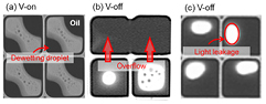
Figure 2. The defects observed from our experiments include (a) oil dewetting patterns, (b) oil overflow, and (c) oil non-recovery. The defect of oil dewetting patterns refers to the oil film being broken up into numerous small oil droplets in the pixel after a certain voltage is applied, resulting in an unstable optical performance and a decrement in transmittance. The defect of oil overflow occurs when the oil phase overflows to the adjacent pixel under an external voltage, and therefore a nonuniform distribution of oil among pixels could be found after the voltage is removed. The defect of oil non-recovery may lead to a decrement in contrast ratio (CR) because of light leakage in the black state when the voltage is removed.
Download figure:
Standard image High-resolution imageTo further improve reliability and optical performance of an EWD device, it is necessary to fully understand the dynamic behaviors of fluids during operation. As opposed to experiments, which would consume massive resources in order to gain sufficient data, numerical models provide an effective tool for predicting device performance. However, very little published work is available on the numerical method of an EWD. For example, Vermeulen et al [19] employed a 2D model to explore the influence of the electrolyte viscosity and the interfacial tension between the oil and electrolyte. However, the proposed 2D model may not provide an accurate simulation of the 3D patterned design such as electrodes with rounded edges or a geometrically nonsymmetric hydrophilic grid [10]. Ku et al [20] provided a 3D model based on the volume of the fluid-continuum surface force (VOF-CSF) to predict the fluid behavior in a single-layered EWD pixel. However, without considering the change in contact angle which results from the EW effect, it is difficult for their simulations to correctly predict the results that happen in practical experiments. Recently, under the OpenFOAM framework, Roghair et al [21] have solved several electro-hydrodynamical problems by incorporating Gauss's law and a charge density transport equation into a VOF multiphase flow code. In their work, the interaction of a fluid–fluid (dielectric–dielectric or dielectric–conductive) interface with an applied electric field is successfully simulated, thus making possible a description of fluid motion in an EWD pixel.
The goal of this work is to develop a more rigorous 3D model that is able to accurately predict the fluid dynamic behavior during the electro–optic process of an EWD, including the break-up and the EW stages when the voltage is switched on and the oil spreading when the voltage is switched off. A general treatment in the switch-on process is proposed here to deal with the fluid motion by coupling the EHD force deduced from the Maxwell stress tensor with the laminar phase field of the oil–water dual phase. To solve the two-phase flow problem, we conduct the phase field method (PFM), which is categorized as an interface capturing approach and has recently emerged as a beneficial tool for incorporating the complex rheology of microstructured fluids [22]. Particularly in the EW stage, as the water has touched the hydrophobic layer, we adopt the idea of Jones et al [15, 23–25] to calculate the change in the apparent contact angle at the contact line. As a consequence, the transient movement of the oil phase with electrical actuation can be successfully simulated. Moreover, the proposed model will be extended to parametrically analyze the effect of interfacial, material, and geometric properties on the defects of an EWD. This defect analysis will help us to implement highly stable EWD applications.
The remaining part of this article is organized as follows. The detailed description of the numerical methods including the governing equations and the boundary conditions will be introduced in the next section. Section 3 will present the results and discussions. Lastly, the conclusions will be given in section 4.
2. Numerical methodology
The objective of the numerical method is to trace the topological changes of the oil–water interface, which moves dynamically in a confined pixel under an external electric field. To this end, the coupling between an electric field and the two fluid phases is considered. The finite element method (FEM) is utilized to solve all of the governing equations including the Cahn−Hilliard equation, the Laplace equation, and the Navier−Stokes equation. The size of a unit pixel (dotted line) used in the computational domain is illustrated in figure 3(a) and the related boundary conditions are displayed in figure 3(b).

Figure 3. Schematic representation of (a) a unit pixel (red dashed line) utilized in simulation, and (b) the relevant boundary conditions used in the phase field, electrostatic, and hydrodynamic calculation.
Download figure:
Standard image High-resolution image2.1. Governing equations
In the phase-field formulation, the moving interface of the oil and water is set as a tiny nonzero-thickness transition region [22]. The physical properties at the interface of the immiscible fluids could be described by functions within this region with the help of a continuous phase-field variable ϕ, which varies from −1 for water to 1 for oil. From the introduced volumetric fractions  and
and  , the physical quantities within the transition region are given as

where ρ, μ, and ε represent the density, viscosity, and dielectric constant of fluids, respectively. In the diffusive-interface picture, the evolution of the interface between oil and water is governed by the Cahn–Hilliard convection equation [26]
where u represents the fluid velocity, M denotes the mobility (or diffusion coefficient), and G is the chemical potential. The mobility can be expressed as  , where χ is the characteristic mobility and
  is the capillary width that scales with the thickness of the diffuse interface in PFM. The value of
  should be determined empirically [22], and we adopt
  in the present simulation, where
  is the oil film thickness. The chemical potential, which is a partial differential of the total free energy with respect to ϕ, could be expressed as
 ![$G=\lambda [-{{\nabla}^{2}}\phi +\phi ({{\phi}^{2}}-1)/h_{\text{PF}}^{2}]$](https://content.cld.iop.org/journals/0960-1317/24/12/125024/revision1/jmm503733ieqn008.gif) , where λ is the energy density parameter. In addition, λ and
, where λ is the energy density parameter. In addition, λ and  are related to the oil–water interfacial tension through the relation:
  .
.
The static electric field in the hydrophobic dielectric layer, hydrophilic grid, oil phase, and water phase, is assumed to be governed by the Laplace equation

where  is the vacuum permittivity,
  is the relative permittivity of the numerical domains including both solid dielectrics and fluids, and V is the electric potential. Under the framework of PFM,
  at the interface between oil and water is also treated as a spatially continuous function, as expressed in equation (1). Here, the assumption of leaky dielectric (no electric charge density) in equation (3) is adopted to simplify the electrostatic equation of the water phase. This assumption, however, would lead to an overestimation (or underestimation) of the electric field in the water phase (or the oil phase). To overcome this problem, we then assign an extremely high value to the dielectric constant within the bulk of water phase. With such a high dielectric constant, the water phase will behave much like a conductive liquid (i.e. the electric field E = −V becomes very small inside the water domain [27]). This nearly conductive behavior of the water phase is compatible with the general treatment in an EW theory, in which the water is usually set to be perfectly conductive and the electric field vanishes within the water [1].
To depict the dynamic movement of the immiscible two-phase flow, the transport of mass and momentum are governed by the incompressible Navier–Stokes equations
where ρ and μ are the density and viscosity of the fluids, which take the form as in equation (1). p, g, Fs, FE respectively denote the pressure, the gravitational acceleration, the volumetric surface tension, and the volumetric electrodynamic force generated by an electric field. Since the Bond number is much smaller than 1 in our simulation problems, the gravitational force in equation (4) can be ignored [1, 28]. In the PFM, FS can be calculated over the computational domain in terms of the chemical potential and phase-field variable by

Obviously, FS approaches zero except those at the diffusive thickness of the oil–water interface. The volumetric electrodynamic force FE, a net effect of an applied electric field acting on the fluids, can be evaluated through the Korteweg–Helmholtz electric force density formulation [29]
where  is the free electric charge density. Since the oil and water are assumed to be dielectric liquids,
  is equal to zero within the bulk. The second term of equation (6), a contribution from the polarization of the fluids, vanishes everywhere except at the interface. The last term of equation (6), the electrostriction force density, can be ignored for incompressible flow. Additionally, by neglecting electrostriction, FE can be expressed by the divergence of the Maxwell stress tensor TM

In component expression,  is written as
where  is the Kronecker delta function, and i, j = x, y, z. By adding the electrodynamic force into the laminar phase field calculation in the simulation, we are able to depict the effect of the electric field on the fluids domain and thus to characterize the dynamic movement of the oil–water interface.
2.2. Boundary conditions
When solving the electrostatic field from the Laplace equation (3), the zero charge condition (i.e. n·D = 0) is adopted for all of the exterior boundaries with the exception of the electrode regions. For the electrode regions, as plotted in figure 4, we specify the voltage V as its applied value  on the patterned electrode and
  on the grounded electrode.
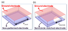
Figure 4. The shape of electrode used in the simulation cases: (a) non-patterned electrode, and (b) semicircle notched electrode.
Download figure:
Standard image High-resolution imageIn the formulation of PFM, the boundary conditions for the solid surfaces (e.g. hydrophobic surface, hydrophilic grid, and top substrate) are considered as wetted walls, and along the surfaces we specify a wetted contact angle  , which is related to ϕ through

where n is the unit vector normal to the wall. Across the wetted wall, the mass flux is zero, and therefore the no-slip boundary condition (i.e. u = 0) is used to associate with the momentum equation (4). In addition, the boundary condition at the four outlets for a unit pixel is chosen as  .
.
The electrowetted contact angle in this model is treated as follows. When the water phase contacts the hydrophobic layer (i.e. the traditional EW effect occurs), the electrically induced force at the contact line, obtained from the surface integral of the Maxwell stress, is expressed as [15, 23–25]
where the subscript 'hyd' denotes the hydrophobic dielectric layer, and d and E represent the thickness and electric field, respectively. Since E vanishes inside the domain of the water phase, the difference of electric potential across the hydrophobic dielectric layer is equal to the external applied voltage (i.e.  ) [24]. Consequently, in view of equation (10) the force balance at the contact line leads to the Lippmann–Young equation:
where  and
and  are the electrowetted contact angle and Young's contact angle of the hydrophobic dielectric layer measured from the water phase, respectively.
Therefore, once the electric field is determined in the voltage-on state by solving the Laplace equation in equation (3), the electrodynamic force generated at the interface can be substituted into the Navier–Stokes equation, equation (4), to drive the fluids. As a result, the topological changes of the oil–water interface with a zero-value contour of the continuous phase field can be traced through the Cahn–Hilliard convection equation (equation (2)).
3. Results and discussions
In this section, we present and discuss the simulation results. The organization of the discussion is as follows. First, the proposed simulation is justified by the use of a theoretical electro–optic model [30]. Second, a complete switch process of an EWD is discussed, and the importance of the electrowetted contact angle on optical performance is highlighted. The third part presents the parametric analysis on various defects, which helps to improve the optical performance and reliability of an EWD. Lastly, according to the defect analysis, a highly reliable EWD is numerically and experimentally realized.
The parameters used in the simulation are listed in table 1, in which the properties of liquids (e.g. density and viscosity) and the interfacial properties (e.g. surface tension of oil and water, contact angle of hydrophobic layer and top substrate) are kept constant. The values of these parameters are identical to those used in our experiments. In addition, in solving the electrostatic equation in equation (3), the dielectric constant for the bulk of the water phase is set to be 2000, instead of the commonly used value of 80. The value 2000 is large enough that the electric field in the water phase becomes very small. Moreover, two types of electrode configurations, i.e. the non-patterned and semicircle notched electrodes as shown in figure 4, are adopted in the simulation.
Table 1. Material, interfacial, and geometric properties used for the simulation.
| Parameters | Quantity | Symbol | value |
|---|---|---|---|
| Material properties | Density of oil |  |
884 kg m−3 |
| Density of water |  |
999.62 kg m−3 | |
| Viscosity of oil |  |
2 cP | |
| Viscosity of water |  |
1.0093 cP | |
| Dielectric constant of oil |  |
2.2 | |
| Dielectric constant of water |  |
80 | |
| Dielectric constant of hydrophobic dielectric layer |  |
6–10 | |
| Dielectric constant of hydrophilic grid |  |
3.9 | |
| Interfacial properties | Surface tension of oil and water |  |
54.5 mN m−1 |
| Contact angle of hydrophobic surface |  |
160° | |
| Contact angle of hydrophilic grid |  |
80–130° | |
| Contact angle of top substrate |  |
30° | |
| Geometric properties | Width of pixel |  |
141–282 μm |
| Width of grid |  |
10–20 μm | |
| Radius of patterned electrode |  |
70.5–141 μm | |
| Thickness of oil film |  |
4–12 μm | |
| Thickness of hydrophilic grid |  |
4–12 μm | |
| Thickness of hydrophobic dielectric layer |  |
1–2 μm |
3.1. Electro–optic performance
The correctness of the numerical approach can be validated by comparing the simulation result of the basic electro–optic behavior of an EWD with that obtained from a physical model [30]. According to this model, the white area fraction (WAF) of a pixel, a measure of electro–optic switching behavior, can be defined by
where  is a normalization factor used to define the threshold value of the base area at zero voltage.
  represents the base area of the spherical oil cap covered on the hydrophobic surface with given applied voltage V, and it can be expressed as
where  is the volume of oil film dosed into the pixel, and
  is the cap angle of the spherical oil cap in the presence of voltage. This angle obeys the equation
which is obtained from the Lippmann–Young equation by assuming that the oil film covers the entire pixel without applying voltage (i.e.  ). Here, C is the capacitance per unit area (F m−2), and η is the EW number, which denotes the ratio between the electrostatic energy per unit area and the interfacial tension. The minus sign of the electrical term in equation (14) indicates that the angle
  is measured from the oil phase rather than from the water phase. In addition, it should be noted that the angle
  is introduced here so that one can intuitively associate the cap angle φ(V) with the base area of the oil droplet in the physical model.
In this simulation we adopt the non-patterned electrode in a 141 μm width pixel, as shown in figure 4(a). The contact angle of grid is set to  (measured from the water phase), which ensures that the oil film in the pixel is geometrically flat in the absence of voltage. In addition, from the self-assembly dosing process used in our experiments, the oil thickness is equal to the grid height of 6 μm.
Figure 5(a) shows the dependence of WAF on the applied voltage for the theoretical (curve) and simulation (symbol) results with different values of capacitance. It can be observed that when  is given as the area of the external circle of the square optical element, i.e.
  (see figure 3(a)), the numerical data points fit well into the curves obtained from the physical model. The inset of figure 5(a) displays the dependence between WAF and η in both the simulation and the physical model. This dependent trend has also been found in a series of experiments [31–33].

Figure 5. (a) Comparison of the numerical (symbols) and theoretical (lines) electro–optic behaviors with different capacities per unit area. The dashed line denotes the critical white area fraction when  . The inset shows the relation between WAF and η. (b) A phase diagram showing the three states separated by the threshold voltage
  (solid line) and the critical voltage
  (dashed line).
Download figure:
Standard image High-resolution imageTo quantitatively characterize the optical range and limitation of an EWD with different C values, a phase diagram is illustrated in figure 5(b), where the threshold voltage  is the voltage required to initiate the movement of the oil film and the critical voltage
  means the voltages required to reach
  (i.e.
(i.e.  ). It is found that the numerical data points in figure 5(a), plotted as symbols, fit well in the phase diagram. Moreover, the electro–optic response of an EWD can be sorted into three states: the black state (i.e.
  ), the grayscale state (i.e.
  with the critical voltage
  ), and the optical saturation state (i.e.
  ). In the black state the electrostatically induced EHD force (which increases as applied voltage increases) is insufficient to break up the oil film. Subsequently, once the water touches the hydrophobic surface (i.e. the EHD force exceeds the surface tension force), the EW effect leading to a grayscale operation then begins.
3.2. Operation processes
In this section, the modeling of the switch process of an EWD is presented and the importance of the electrowetted contact angle on optical performance is discussed.
3.2.1. Switch-on process.
For practical EWDs, a patterned electrode is required to drive the oil film toward a preferred direction. The rounded pattern is commonly used to prevent electrical breakdown at the electrode edges [10]. Here, a semicircle notched electrode with a width of 70.5 μm is adopted in the simulation, as sketched in figure 4(b). In addition, the pixel width is set as 141 μm, and the thickness and the dielectric constant of the hydrophobic dielectric layer are  2 μm and
  6, respectively. The applied voltage V is given as 40 V, which is sufficient to break up the oil film according to the analysis in section 3.1.
In the simulation, we set the wetted contact angle  at the hydrophilic grid, and thus the oil–water interface is initially flat in the confined pixel. Figure 6 shows the simulated evolution of the oil phase concentrated to the corner from a film to a droplet during the switch-on process of about 0.45 ms. Obviously, the choice of the patterned electrode determines the direction of movement of the oil phase toward the corner.

Figure 6. Switching evolution of oil phase concentrated from a film to a droplet with voltage of  from t = 0 to 0.45 ms.
Download figure:
Standard image High-resolution imageThe time history of the electric field distribution in the diagonal section of the numerical domain (see figure 7(a)) is illustrated in figure 7(b). This result enables us to distinguish the break-up and the EW stages in the switch-on process. At the beginning of the break-up stage (t = 0 ms), the water phase does not touch the hydrophobic surface and the largest magnitude of the electric field is found at the oil phase, as shown in figure 7(b). Hence, corresponding to the electric filed, a downward (toward the oil phase) volumetric electro-dynamic force FE calculated through equation (7) appears at the oil–water interface, as shown in figure 7(c). In the EW stage (from t = 0.05 to 0.45 ms), which begins from the time the water phase is in contact with the hydrophobic surface, a strong electric field can be found in the dielectric layer. This contact gives rise to a significant change in the oil phase contact angle. The electric field in the vicinity of the contact line within the oil phase is found to be relatively high in both the vertical and horizontal directions, as respectively shown in figures 7(c) and (d).
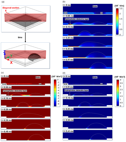
Figure 7. (a) Diagonal section of the numerical domain. Simulated distribution in the diagonal section from t = 0 to 0.45 ms for (b) the magnitude of the electric field, (c) the volumetric electrodynamic force in the vertical direction, and (d) the volumetric electrodynamic force in the horizontal direction. Note that the curved line of the oil–water interface is identified by tracing the zero-value contour of the phase-field function.
Download figure:
Standard image High-resolution image3.2.2. Switch-off process.
After the oil film is contracted to the pixel corner, the switch-off process begins as soon as the voltage is removed. In this simulation, the initial phase field for the switch-off process is set as the final phase field of the switch-on process at t = 0.45 ms. Figure 8 shows the evolution of the oil phase from a droplet back to a film. The value of response time for the switch-off process is  ~ 5.6 ms. We also find that the spreading speed of the oil phase at the beginning of the stage (from t = 0 to 0.3 ms) is relatively high, which is consistent with the experimental observation [7].
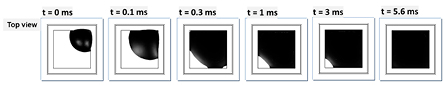
Figure 8. Switching evolution of oil phase spreading from a droplet to a film in the absence of voltage from t = 0 to 5.6 ms.
Download figure:
Standard image High-resolution image3.2.3. Effect of electrowetted contact angle.
Owing to the force balance at the contact line in equation (11), the contact angle of the water phase should be deviated from  in the simulation of the EW stage. When the oil is completely concentrated in the patterned pixel corner, the contact angle of the water phase
  (i.e. the angle measured from the oil phase is
  ) is observed, as shown in figure 9(a). This angle agrees with the value calculated through the Lippmann–Young equation (=
 ) [1]. However, if we try to keep a constant contact angle (
 ) at the hydrophobic surface, the contact angle of the water phase is found to be
  (i.e. the angle measured from the oil phase is
  ) as shown in figure 9(b). In addition, figure 9(c) shows the time evolution of WAF during the switch-on process, and it can be seen that the highest WAF for the case of electrowetted contact angle is larger than that for the case of constant contact angle. This tells us that a correct description of the contact angle has an influence on the accuracy of the numerical model when we measure the optical performance of an EWD, such as the response time or the transmittance.

Figure 9. Contact angle measurements in the diagonal section of the numerical domain after the electrical actuation of an oil film. Case (a) considers the electrically induced force  at the contact line, and case (b) uses a constant contact angle as a boundary condition on the hydrophobic surface. (c) The time evolution of WAF for the two cases.
Download figure:
Standard image High-resolution image3.3. The effect of the hydrophilicity of the grid on optical performance
The hydrophilicity of the pixilating grid is a key factor that is associated with several types of defects observed in EWDs, such as oil dewetting patterns [10] and oil overflow [17]. To avoid these defects, a large number of tests should be conducted to collect sufficient data on the contact angles of the grid  that cause the defects. Such collection, however, is time-consuming and some angles cannot be easily obtained from experiments. Our simulation model provides a useful alternative so that a parametric analysis can be made. Here, we choose two pixel sizes
  = 141 and 282 μm with their respective oil thickness
  = 6 and 12 μm, and the other parameters are the same as those in section 3.2.
3.3.1. Oil dewetting patterns.
The influence of the contact angle of the hydrophilic grid  on EWD optical performance is demonstrated in figure 10, where the symbols (
 ,
,  ,
,  ) represent the oil film thickness, the pixel width, and the grid width, respectively. It can be seen that WAF (solid circle) decreases as
  increases for both pixel sizes when
  . If we keep increasing
  , up to
  for example, a hole is found in the center of the pixel (see the right inset of figure 10), which will cause a lower value of WAF. Furthermore, we notice that the dewetted oil droplets, i.e. the residue droplets, can still be found in the pixel if
  . This is attributed to the fact that when
  the initial profile of the oil film in the pixel presents the concave shape instead of a flat or spherical one. Consequently, once a voltage is exerted, the oil film will be easily broken up at its center (i.e. the thinnest region), resulting in the occurrence of multiple droplets (see the middle inset of figure 10). The simulation result agrees with the experimental observation, shown diagrammatically in the photo in figure 2(a), in which the contact angle of the hydrophilic grid
  is equal to
  . In contrast, when
  , the oil film is successfully contracted into a single droplet, thus giving relatively high values of WAF, shown in the left inset of figure 10. Therefore, the condition
  is suggested such that the occurrence of oil dewetting patterns in the pixels can be avoided and a better optical performance can be obtained for the EWD.
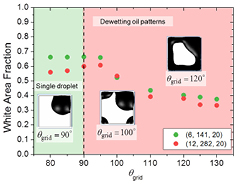
Figure 10. Effect of the contact angle of hydrophilic grid ( ) of an EWD on WAF for the two types of geometric properties: (
 ,
,  ,
,  ), where
  is the angle measured from the water phase. When
  , the single droplet as illustrated in the inset can be found when the voltage is applied. However, when
  , the dewetting oil patterns can be observed.
Download figure:
Standard image High-resolution image3.3.2. Oil overflow.
The hydrophilicity of the grid also plays a critical role in the occurrence of oil overflow. To quantify this undesirable defect, we introduce a dimensionless parameter  , where
  is the furthest distance the oil can move on a grid. When α is greater than 0.5, the oil phase crosses the border of a unit pixel and overflows to the adjacent pixels. In this simulation, the same parameters as those in section 3.3.1 are adopted.
Figure 11 presents the effect of  on α. We see that α increases as
  increases for all of the simulation cases. With the setting of (
 ,
,  ,
,  ) = (12, 282, 20), it is found that α exceeds 0.5 when
  . This explains the experimental finding of oil overflow in figure 2(b), where the contact angle of the hydrophilic grid
  was used. The simulation also indicates that the higher the oil volume is dosed into the pixel, the lower the contact angle of the grid required to avoid oil overflow. From the simulation, we suggest that the contact angle for the cases (6, 141, 20), (6, 141, 10), (12, 282, 20), and (12, 282, 10) to avoid oil overflow should be less than
  ,
,  ,
,  , and
, and  , respectively.
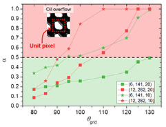
Figure 11. Effect of  on α with different geometric properties (
 ,
, ,
, ). It is found that α increases as
  increases. When α exceeds 0.5 (dashed line), the oil overflow defect occurs as shown in the inset, where the red dashed square represents the unit pixel.
Download figure:
Standard image High-resolution image3.4. The effect of oil thickness on oil non-recovery
It is expected that an oil droplet should recover the whole pixel area as soon as the applied voltage is removed. Some factors are thought to be associated with the oil non-recovery defect, such as the hydrophobicity of the dielectric layer [10, 32] and the oil thickness. The latter factor is addressed in this section from a theoretical viewpoint followed by a simulation.
Consider a spherical oil cap with volume  , whose base radius
  , i.e. the radius of the circular interface between the cap and the solid surface, can be expressed as
where φ is the contact angle of the spherical oil droplet, which is related to the Young's contact angle of hydrophobic dielectric surface  through
  . Based on the self-assembled oil dosing process [34] that is conducted in our experiment, the volume of oil film dosed into the square shaped pixel should be equal to
  . Now let's assume that
  should be larger than a threshold radius
  such that the oil film could successfully recover the pixel at zero voltage. The selection of
  is a result of the experimental observation. In view of the assumption and equation (15), a criterion for the oil recovery is found to be

Accordingly, we are able to construct a phase diagram for  and
and  in figure 12(a), in which the dashed lines are obtained from equation (16) with two sizes of pixel. This phase diagram helps us to predict the recoverable condition in terms of oil thickness and contact angle of the hydrophobic dielectric layer. For example, if
  is adopted, the threshold oil film thicknesses for the pixel sizes
  and 282 μm will then be about 5 and 10 μm, respectively. This could explain why the thicknesses we adopted for the simulations reported in the previous sections are 6 and 12 μm with the pixel sizes of 141 and 282 μm, respectively. In addition, the oil non-recovery observed from our experiment as shown in the diagrammatical photo in figure 2(c), where the oil thickness
  = 8 μm, the pixel size
  = 282 μm, and the contact angle of the hydrophobic layer
  were used, agrees with the theoretical prediction.

Figure 12. (a) A phase diagram of the contact angle of the hydrophobic dielectric layer ( ) versus oil film thickness (
 ) for various pixel sizes (
 ). Each dashed line, which separates the domains of oil recovery and oil non-recovery, is plotted according to the theoretically derived equation (16). The symbols o and x, obtained from the simulation with the use of
  , refer respectively to the oil recoverable and non-recoverable results. The time evolutions of WAF in both switch-on (solid line) and switch-off (dashed line) processes are displayed for (b)
  = 6 μm, where the oil droplet is able to fully re-cover the pixel, and for (c)
  = 4 μm, where the oil fails to fully re-cover the pixel.
Download figure:
Standard image High-resolution imageIn order to be compatible with the theoretical analysis, a simulation is performed in which we adopt 141 μm pixel and the non-patterned electrode. The contact angles of the grid and the hydrophobic dielectric layer are fixed at  and
and  , respectively. To investigate how the oil thickness
  influences the oil recovery, five different oil thicknesses
  = 3 ~ 7 μm are used. As shown in figure 12(a), when
  5 μm, the oil in the 141 μm pixel (symbol o) is recoverable after the voltage is removed. However, when
  4 μm, the oil non-recovery defect is found (symbol x). The time evolutions of WAF in the process of switch-on (solid line) and switch-off (dashed line) for
  = 6 μm and
  = 4 μm are shown in figures 12(b) and (c), respectively. The above result indicates that as the pixel size and the hydrophobicity of the hydrophobic layer are specified, there exists a critical value of oil thickness, above which a complete spreading can be achieved. This can also be experimentally verified as illustrated in figure 2(b), where part of the oil in the bottom pixels overflows into the upper pixels, leading to the oil non-recovery defect in the bottom pixels when the voltage is turned off. This oil non-recovery defect comes from the fact that the remaining volume of the oil in the pixel is lower than the critical value.
3.5. Highly reliable EW display
In this section, we demonstrate how a highly reliable EWD is realized. As stated above, the requirement for the contact angle of the grid to avoid both oil dewetting patterns and oil overflow is  . However, it is very challenging in a real test to let the hydrophilic grid adhere firmly onto the hydrophobic surface [10]. Therefore, the hydrophilic grid of contact angle
  is suggested. As for the 282 μm pixel size, the thickness of the grid is chosen as 12
  so that the defect of oil non-recovery can be avoided. In what follows, the fabrication processes of the EWD are briefly introduced, and then the electro–optic performance of the EWD is presented in experimental and numerical terms.
3.5.1. Fabrication processes.
Our fabrication processes are described as follows. First, the  (ITO) film with thickness 100 nm is deposited on the top glass substrate by sputtering, and then patterned using the photolithography technique. Second, two dielectric layers, 100 nm of SiNx (
 ) and 50 nm of SiO2 (
 ), are respectively deposited on the ITO film using plasma-enhanced chemical vapor deposition (PECVD). Third, the 100 nm hydrophobic layer (fluoropolymer) is coated on the dielectric layer using the spin coating method. After prebake of the fluoropolymer, the sample is oxygen plasma treated to improve the wettability and adhesion between the hydrophilic grid (negative photoresist) of contact angle
  and the hydrophobic layer of contact angle
  By using the photolithography process again, the hydrophilic grid of 20
  width with a square pattern (
 μm) is fabricated. As noted above, the thickness of the hydrophilic grid is chosen as 12
  . Then, the black oil is dosed into the pixels using the dip coating method [34]. Finally, the conductive liquid is dosed to cover the oil film, and the top glass substrate with ITO film is used to assemble the EWD panel.
3.5.2. Electro–optic performance: simulation and experiment.
The electro–optic performance (η versus WAF) of the designed EWD is experimentally and numerically presented in figure 13. In the experiment, the threshold voltage  is found to be 2.8 V, and thus the corresponding η is about 0.008. As shown in the inset of figure 13, the successful switch-on process without oil overflow and without dewetted droplets (i.e. the oil was fully contracted to the pixel corner from a film to a droplet) is observed in both the simulation and the experiment. To summarize, the agreement of the electro–optic performance between the experiment and the simulation in figure 13 lies in a correct description of the electro/dual phase coupling and the change in the apparent contact angle at the contact line in the simulation.

Figure 13. Electro–optic behavior of an EWD obtained from the experiment (O) and the simulation (X). Insets: the oil was successfully contracted to the pixel corner from a film to a droplet in both the experiment and the simulation.
Download figure:
Standard image High-resolution image
4. Conclusions
In this work, a 3D model based on the coupling between the EHD force and the laminar phase field of the oil–water dual phase is proposed to simulate the electro–optic response in a single-layered EWD pixel. Through this model, we have successfully simulated the complete process of the electro–optic operation, including the break-up and EW stages when the voltage is switched on and the oil spreading when the voltage is switched off. The EW effect involving an electromechanical force and a reduction of the contact angle can thus be well delineated. By doing so, the simulated electro–optic performance (voltage versus WAF) is found to agree well with that obtained from the experiment. Through the numerical and theoretical analyses of the defects of oil dewetting patterns, oil overflow, and oil non-recovery, a highly stable EW display is successfully realized. Furthermore, the proposed model can be extended to explore the effect of the material, interfacial, and geometric properties on the EWD performance. Therefore, we believe that the rigorous 3D simulation provides an effective tool to accurately predict the dynamic behavior and electro–optic performance of an EWD.
Acknowledgments
This work was supported by the ROC National Science Council under grants NSC-102-2221-E-002-221 and MOST-103-2221-E-002-070.