Abstract
Harvesting flow energy by exploiting transverse galloping of a bluff body attached to a piezoelectric cantilever is a prospective method to power wireless sensing systems. In order to better understand the electroaeroelastic behavior and further improve the galloping piezoelectric energy harvester (GPEH), an effective analytical model is required, which needs to incorporate both the electromechanical coupling and the aerodynamic force. Available electromechanical models for the GPEH include the lumped parameter single-degree-of-freedom (SDOF) model, the approximated distributed parameter model based on Rayleigh–Ritz discretization, and the distributed parameter model with Euler–Bernoulli beam representation. Each modeling method has its own advantages. The corresponding aerodynamic models are formulated using quasi-steady hypothesis (QSH). In this paper, the SDOF model, the Euler–Bernoulli distributed parameter model using single mode and the Euler–Bernoulli distributed parameter model using multi-modes are compared and validated with experimental results. Based on the comparison and validation, the most effective model is employed for the subsequent parametric study. The effects of load resistance, wind exposure area of the bluff body, mass of the bluff body and length of the piezoelectric sheets on the power output are investigated. These simulations can be exploited for designing and optimizing GPEHs for better performance.
Export citation and abstract BibTeX RIS
1. Introduction
Wireless sensing systems have been widely used in structural health monitoring. Due to the inconvenience and high cost of the replacement of batteries, the development of self-powered sensor nodes by harvesting ambient energy has been researched extensively in the past few years. Ambient mechanical vibrations can be converted to electricity via electrostatic [1], electromagnetic [2], piezoelectric [3] and magnetostrictive [4] mechanisms, among which piezoelectric transduction has attracted much interest because of its high power density and non-reliance on external magnetic field or initial voltage. Many studies have been conducted on energy harvesting using piezoelectric materials [5–11]. These studies mainly focus on converting the pre-existing structural vibrations into electricity. However, piezoelectric energy harvesting from light winds has received only limited attention.
When structures are subjected to wind flows, aeroelastic instabilities such as vortex-induced vibrations, galloping, flutter and buffeting may occur given specific conditions. The energy of such wind-induced vibrations can be beneficially converted into electricity via the piezoelectric transduction mechanism. Many studies have been conducted on harnessing wind energy by exploiting these aeroelastic instabilities [12–39].
Some researchers proposed energy harvesters with flapping wings to convert aeroelastic flutter vibrations into electricity [12–22]. Bryant and Garcia [15] analyzed the flutter boundary and limit cycle behavior of a piezoelectric bimorph with a rigid flap connected to the tip. A peak power of 2.2 mW was obtained at 7.9 m s−1. Erturk et al [16] investigated the potential of harvesting energy from aeroelastic vibrations with a piezoaeroelastic airfoil. Linear analysis of power generation at the flutter boundary was performed. Different from the use of flapping wings, several other devices with alternative structural designs were proposed to extract power from aeroelastic instabilities. Li et al [23] developed a bio-inspired piezo-leaf architecture which generated electricity by cross-flow fluttering motion, gaining a peak power of 600 μW. Kwon [24] experimentally investigated the power output of a T-shaped piezoelectric cantilever, and obtained the empirical formula to calculate the cut-in wind speed. Wind energy harvesters employing vortex-induced vibrations were also frequently investigated, which were usually designed as a linear mechanical resonator with a cylinder placed windward [25–29]. Maximum power output was achieved when the frequency of vortex shedding approached the natural frequency of the harvester. Akaydin et al [28] tested the efficiency of such a harvester and obtained a maximum power of 0.1 mW at 1.192 m s−1. The main constraint of such harvesters is the narrow wind speed range for effective power generation. Jung and Lee [30] studied the performance of a harvester exploiting wake galloping with two paralleled cylinders. Electromagnetic induction was employed rather than piezoelectric transduction. Recent progress on wind energy harvesting also includes a damped cantilever pipe carrying flowing fluid proposed by Elvin and Elvin [31] and a harmonica-type aeroelastic micropower generator developed by Bibo et al [32].
Translational galloping is another aeroelastic instability phenomenon giving rise to transverse oscillations normal to the wind flow direction in structures with weak damping, when the wind speed exceeds a critical value. It is a better choice to obtain structural vibrations for energy harvesting purposes compared to the vortex-induced vibrations and flutter, due to the advantages of large oscillation amplitude and the ability of oscillating in an infinite range of wind velocities [36, 45]. Translational galloping was first analyzed by Den Hartog [40], and a criterion for galloping stability was introduced. Many researchers have studied the effect of various parameters on the galloping stability of different structures, including the angle of attack, cross-section geometries, flow turbulence, Reynolds number, etc [41–45]. Barrero-Gil et al [33] theoretically analyzed the potential use of transverse galloping to harvest energy using an SDOF model. No specific design of harvester device was proposed. Abdelkefi et al [34] considered a galloping piezoelectric energy harvester (GPEH) with a square prism as the bluff body, and investigated the effects of Reynolds number and load resistance on the threshold of galloping and the level of harvested power. They further theoretically compared the performance of different cross-section geometries of the bluff body for GPEHs with linear and nonlinear analysis [35]. An SDOF model was employed for these two studies, with the value of electromechanical coupling manually specified. Yang et al [36] experimentally studied the influence of cross-section geometry on the performance of GPEHs, and validated the established SDOF model with the experimental results. Sirohi and Mahadik [37] studied a GPEH consisting of two piezoelectric cantilevers connected to a prism with an equilateral triangular section. They also developed another GPEH using a composite piezoelectric cantilever connected in parallel to a prism with D-shaped section [38]. For these two harvesters, an approximated distributed parameter model based on energy method (Rayleigh–Ritz type of discretization) was used. Abdelkefi et al [39] employed the harvester design of Sirohi and Mahadik [37] and further studied the influence of load resistance on the threshold of galloping and harvested power level with a Euler–Bernoulli distributed parameter model. Single mode (fundamental mode) was considered in their analysis. In all the analytical models mentioned above, the aerodynamic forces were formulated based on quasi-steady hypothesis (QSH). Each model method has its own merits, such as the simple form and ease of application of the SDOF model, and the accuracy of the distributed parameter models. Although many studies have been conducted on the issues of the electromechanical models for vibration piezoelectric energy harvesters under base excitation [46, 47], more work needs to undertaken on the modeling and better design of GPEHs which incorporate the aerodynamic forces.
This paper compares different modeling methods for GPEHs. The SDOF model established in the preceding study [36], Euler–Bernoulli distributed parameter model using single mode and multi-modes are considered followed by experimental validation. The merits, disadvantages and applicability of these methods are discussed. Subsequently, employing the most effective model from the comparison, parametric study is performed to study the effects of load resistance, wind exposure area of the bluff body, mass of the bluff body and length of the piezoelectric sheets on the electroaeroelastic behavior (cut-in wind speed and power output level) of GPEHs. The results can be exploited for designing and optimizing GPEHs for better power output performance.
2. The mechanism of galloping
Translational galloping is a self-excited phenomenon giving rise to large amplitude oscillations of a bluff body when subjected to wind flows. Assume that a bluff body is elastically mounted as shown in figure 1. The governing equation of the galloping motion can be written as

where w is the vertical position of the bluff body in z direction; M is the mass of the bluff body; C is the damping coefficient; K is the stiffness of the system and Fz is the aerodynamic force. The overdot denotes differentiation with respect to time t. Fz can be expressed as [45]

where ρa is the air density; Stip is the exposure area facing the flow; U is the wind speed and CFz is the total aerodynamic force coefficient in z direction. QSH is employed here, which considers that the aerodynamic force during galloping oscillation is equal to that when the bluff body is steady with the corresponding angle of attack. This hypothesis is applicable when the oscillation is slow enough, which requires that the characteristic timescale of the flow is much smaller than the characteristic timescale of the oscillation, corresponding to the character of the galloping phenomenon. The larger the wind speed, the safer it is to use QSH. QSH has been confirmed to be able to successfully model galloping in many studies [40, 41, 45]. For a specific cross-section geometry, CFz is a function of the angle of attack α (figure 1), and can be determined through experiments [40–45]. It is common to express CFz as a polynomial expansion as

where Ar are empirical coefficients for the polynomial fitting [33, 45]. If the bluff body undergoes only translational oscillation without rotation, α can be expressed as
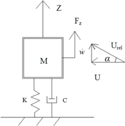
Figure 1. Schematic of a bluff body undergoing galloping.
Download figure:
Standard image High-resolution imageSubstituting equations (2)–(4) into equation (1), and dividing both sides by M yields
where ζ is the damping ratio and ωn is the natural frequency of the system. The aerodynamic force can be considered as an effective nonlinear damping as shown in equation (5), rendering the galloping 'self-excited'. The criterion for galloping instability, which is identified by Den Hartog [40], is expressed as
The criterion requires A1 > 0. For arbitrarily small  , the system is controlled by the linear damping
  , which is positive, thus the oscillations will be damped to the zero equilibrium. When U increases and exceeds a certain value, the linear damping becomes negative, giving rise to galloping oscillations of the bluff body (Hopf bifurcation). When
  is large enough due to the increasing oscillation amplitude, the nonlinear damping
 ![$\frac{1}{2 M}{\rho }_{\mathrm{a}}{S}_{\mathrm{tip}}U[{\sum }_{r=2,\ldots }{A}_{r}\left (\frac{\dot {w}}{U}\right )^{r-1}]$](https://content.cld.iop.org/journals/0964-1726/22/12/125003/revision1/sms483550ieqn76.gif) should be taken into account which makes the overall damping non-negative. Limit cycle oscillation will occur when the damping reaches zero. Due to the self-excited and self-limiting characteristics of galloping, it is a prospective energy source for energy harvesting.
should be taken into account which makes the overall damping non-negative. Limit cycle oscillation will occur when the damping reaches zero. Due to the self-excited and self-limiting characteristics of galloping, it is a prospective energy source for energy harvesting.
3. Comparison of modeling methods for a galloping piezoelectric energy harvester
A typical GPEH is usually designed as a piezoelectric cantilever attached to a bluff body at the free end, as shown in figure 2. The bluff body, which is of a specific cross-section, oscillates in the direction normal to the incoming flow due to galloping. Two piezoelectric sheets are bonded to each side of the substrate beam, generating electricity from the mechanical strain which is developed due to the bluff body oscillation. The analytical model of a GPEH should consider both the electromechanical coupling effect and the aerodynamic force acting on the bluff body. Commonly used models for GPEHs include the SDOF model, the approximate distributed parameter model with Rayleigh–Ritz type of discretization, and the Euler–Bernoulli distributed parameter model with exact analytical mode shapes. The main difference between these models lies in the representation of the electromechanical coupling term. This section will compare the merits, disadvantages and applicabilities of the lumped parameter and distributed parameter models. The aerodynamic forces are all formulated based on quasi-steady hypothesis, although their representation formulas vary due to the different mechanical parameters employed in the corresponding electromechanical equations. The power storage technique is not considered in this paper, so the simple electric circuit only consists of an external resistive load RL.
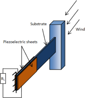
Figure 2. Schematic of a typical GPEH.
Download figure:
Standard image High-resolution image3.1. SDOF model
In the preceding study, a simple SDOF model was established to simulate the electroaeroelastic behavior of a GPEH [36]. In that model, the harvester was considered to oscillate close to the fundamental frequency, which was confirmed with visual observation during the experiment. The governing equations are given as
where w(L,t) is the displacement of the bluff body in the direction normal to the wind flow; Ceff and Keff are the effective damping and stiffness of the harvester; V(t) is the generated voltage across RL; CP is the total capacitance of two piezoelectric sheets with parallel connection; Θ is the electromechanical coupling term; h and ltip are the frontal dimension and length of the bluff body, the product of which equals Stip; and Meff is the effective mass approximated as Meff = 33/140Mb + Mtip, where Mb and Mtip are the mass of the cantilever and the bluff body. Θ is determined easily though experiments by

where ωnoc and ωnsc are the open circuit and short circuit resonant frequencies of the harvester. CFz is expressed as in equation (3), and the attack angle is modified to  , where w'(L,t) is the rotation angle at the free end due to the deflection of the beam, approximated as w'(L,t) = 3w(L,t)/2L.
By defining a state vector X,

the governing equations can be written in the state space form as
where 2ζωn = Ceff/Meff and ωn = ωnsc. Equation (10) can then be numerically solved in MATLAB using a solver like ode45 to determine the vibration response of the beam, cut-in wind speed, and generated voltage across RL. The average power Pave is related to the root mean square (RMS) voltage VRMS as  .
.
3.2. Euler–Bernoulli distributed parameter model
Distributed parameter electromechanical models based on Euler–Bernoulli beam theory have been studied extensively for vibration piezoelectric energy harvesters with base-excitations [5, 46, 47]. For a GPEH, the electromechanical equations are developed based on similar assumptions: (a) the Euler–Bernoulli beam assumptions are applied to the composite beam; (b) the perfectly conductive electrodes fully cover the top and bottom surfaces of the piezoelectric sheet inducing uniform electric field through the thickness; (c) only the z-direction vibration (transverse vibration) is considered; (d) the damping mechanisms including the internal strain rate damping and external air damping satisfy the proportional damping criterion. The schematics of the GPEH showing the coordinate directions and the cross-section of the composite beam are presented in figure 3. We consider the electrically parallel connection for the two piezoelectric sheets. The coupled governing equations for the GPEH can be written as [5, 39]
where w(x,t) is the transverse deflection of the beam in z direction; δ(x) is the Dirac delta function; cs and ca are the coefficients of strain rate damping and air damping; m(x) is the distributed mass of the beam, being expressed as m(x) = ρshsbs for 0 < x < x1 and x2 < x < L, and m(x) = ρshsbs + 2ρphpbp for x1 < x < x2, where ρs,hs and bs are the mass density, thickness and width of the substrate, respectively, ρp,hp and bp are the corresponding terms of the piezoelectric sheet, and x1 and x2 are respectively the starting and ending positions of the piezoelectric sheets along the beam; YI(x) is the bending stiffness of the composite beam expressed as  for 0 < x < x1 and x2 < x < L, and
 ![$Y I(x)={Y}_{\mathrm{s}}{b}_{\mathrm{s}}{h}_{\mathrm{s}}^{3}/1 2+2{Y}_{\mathrm{p}}{b}_{\mathrm{p}}[({h}_{\mathrm{p}}+{h}_{\mathrm{s}}/2)^{3}-{h}_{\mathrm{s}}^{3}/8]/3$](https://content.cld.iop.org/journals/0964-1726/22/12/125003/revision1/sms483550ieqn138.gif) for x1 < x < x2, where Ys and Yp are the Young's modulus of the substrate and piezoelectric material, respectively; θ is the piezoelectric coupling term given by θ =− Ypd31bp(hp + hs), where d31 is the piezoelectric constant; and Cp is the total capacitance as in the SDOF model, being given by
for x1 < x < x2, where Ys and Yp are the Young's modulus of the substrate and piezoelectric material, respectively; θ is the piezoelectric coupling term given by θ =− Ypd31bp(hp + hs), where d31 is the piezoelectric constant; and Cp is the total capacitance as in the SDOF model, being given by  ((x2 − x1) equals the length of the piezoelectric sheets Lp), where
  is the permittivity at constant strain. As in the SDOF model, Fz is the aerodynamic force due to galloping.

Figure 3. (a) Top view of the considered GPEH, and (b) cross-section of the composite beam, for x1 < x < x2.
Download figure:
Standard image High-resolution imageThe transverse deflection w(x,t) can be represented as
where ϕr(x) is the mass normalized mode shape for the rth mode of the corresponding undamped free vibration problem, and ηr(t) is the modal coordinate. Erturk and Inman [5, 46, 47] presented the procedure for the exact analytical solution of ϕr(x) for a cantilever fully and uniformly covered with piezoelectric materials. As for a cantilever beam which is partially covered by piezoelectric sheets (the case for our prototype in the experiment), Abdelkefi et al [39] developed the Euler–Bernoulli distributed parameter model by deriving the exact analytical mode shape function to analyze the electroaeroelastic behavior of a GPEH. Yet such an analytical solution for the segmented mode shapes is quite cumbersome. Single mode (fundamental mode only) was considered in their analysis. In this paper, we obtain ϕr(x) and  easily by the finite element method in Matlab. Hermite cubic functions are employed as the interpolation functions for the beam element.
Fz is still in the form as in the SDOF model (equation (7)), but the attack angle is here expressed in modal coordinates,

Subsequently, introducing equations (12) and (13) into equation (11) yields the coupled governing equations in modal coordinates,
where ζr is the modal mechanical damping; ωr is the undamped natural frequency of the rth vibration mode; and χr is the modal electromechanical coupling term written as ![${\chi }_{r}=\theta [{\phi }_{r}^{\prime}({x}_{2})-{\phi }_{r}^{\prime}({x}_{1})]$](https://content.cld.iop.org/journals/0964-1726/22/12/125003/revision1/sms483550ieqn169.gif) . Before proceeding to solve equation (14), a short explanation of how to evaluate ζr is presented here. As mentioned in assumption (d), the mechanical damping which includes the internal strain rate damping and external air damping is treated with the proportional damping (Rayleigh damping) assumption. For a uniform piezoelectric beam of which the flexural rigidity YI and mass per unit length m are both uniformly distributed [5, 46, 47], ζr can be simply expressed as ζr = csIωr/2YI + ca/2mωr. Once the damping ratios for two separate vibration modes are known, the two unknown constant damping coefficients cs and ca can be mathematically calculated. Yet for a non-uniform piezoelectric beam which is partially covered by piezoelectric sheets as in our case, cs and ca are no longer constant along the beam length. Whereas we can still assume that csI(x) and ca(x) are stiffness proportional and mass proportional, respectively, and obtain two constant values of (csI/YI)ave and (ca/m)ave. However, to avoid the calculation of these coefficients as well as the inaccuracy caused by the proportional damping assumption, we can obtain ζr experimentally using the frequency response function (FRF) obtained in base-vibration condition [48] and proceed to numerical solution of equation (14) for the mechanical and electric responses of the GPEH.
. Before proceeding to solve equation (14), a short explanation of how to evaluate ζr is presented here. As mentioned in assumption (d), the mechanical damping which includes the internal strain rate damping and external air damping is treated with the proportional damping (Rayleigh damping) assumption. For a uniform piezoelectric beam of which the flexural rigidity YI and mass per unit length m are both uniformly distributed [5, 46, 47], ζr can be simply expressed as ζr = csIωr/2YI + ca/2mωr. Once the damping ratios for two separate vibration modes are known, the two unknown constant damping coefficients cs and ca can be mathematically calculated. Yet for a non-uniform piezoelectric beam which is partially covered by piezoelectric sheets as in our case, cs and ca are no longer constant along the beam length. Whereas we can still assume that csI(x) and ca(x) are stiffness proportional and mass proportional, respectively, and obtain two constant values of (csI/YI)ave and (ca/m)ave. However, to avoid the calculation of these coefficients as well as the inaccuracy caused by the proportional damping assumption, we can obtain ζr experimentally using the frequency response function (FRF) obtained in base-vibration condition [48] and proceed to numerical solution of equation (14) for the mechanical and electric responses of the GPEH.
Assume the first nth modes are considered. Again, we introduce the state vector,
The governing equations can then be written in the state space form as
Like the SDOF model, equation (16) can be solved in MATLAB using ode45. Two cases with different numbers of modes employed will be considered in section 4. Firstly, we only consider the fundamental mode by letting n equal 1 in equation (16), since a GPEH is oscillating near its fundamental frequency [37, 38]. Secondly, in order to get a more accurate expression for the galloping aerodynamic force, we take into account the first three modes (n = 3) to investigate how the higher modes influence the overall responses of a GPEH.
4. Model comparison based on experimental validation
4.1. Experimental setup
A prototype device is fabricated and tested in the wind tunnel following the same experimental setup procedure as the preceding study [36], and the measured results are presented to validate the aforementioned SDOF and distributed parameter models. The effectiveness of the models is compared based on the agreement between their predictions and experiments. The cantilever beam is the same as the one in [36], which is composed of an aluminum substrate with two piezoelectric sheets (DuraAct P-876.A12 from Physik Instrumente) bonded to each side of the root, being connected in parallel with the total capacitance Cp = 180 nF. A metal support is employed to fix the root of the cantilever in the wind tunnel. A bluff body is attached to the free end. According to the preceding experimental study on the cross-section geometry of the bluff body [36], a square section is employed, for its better performance than other geometries in the laminar flow, with the lowest cut-in wind speed and the largest output power. Three Configurations are tested in the wind tunnel with different bluff body properties for adequate model comparisons. The properties of the beam and piezoelectric sheets are listed in table 1, while those of the bluff body are shown in table 2. The prototype and the installation in the wind tunnel are shown in figure 4(a). Prior to the wind tunnel test, some parameters such as ζ,ωnsc and ωnoc need to be measured under base-excitation. The damping ratio ζ for the SDOF model is the same as ζ1 in the distributed parameter model. For Configuration 1, ζ1 = 0.005 [36], ζ2 = 0.015 and ζ3 = 0.034; for Configuration 2, ζ1 = 0.008,ζ2 = 0.019 and ζ3 = 0.041; for Configuration 3, ζ1 = 0.004,ζ2 = 0.012 and ζ3 = 0.031. During the wind tunnel test, the wind speed is measured by a Pitot tube anemometer, and the voltage across the load resistance is measured by the NI 9229 data acquisition module. The overall experimental setup is presented in figure 4(b).
Table 1. Parameters of cantilever beam and piezoelectric sheets [36].
| Properties | Beam | Piezoelectric sheets |
|---|---|---|
| Length (mm) | 150 | 61 |
| Width (mm) | 30 | 30 |
| Thickness (mm) | 0.6 | 0.5 |
| Material | Aluminum | DuraAct P-876.A12 |
| Mass density (kg m−3) | 2700 | 3825 |
| Capacitance (nF) | — | 90 |
| Young's modulus (GPa) | 69 | 23.3 |
| Piezoelectric constant d31 (pm V−1) | — | −174 |
Table 2. Parameters of the bluff body for the three Configurations.
| Properties | Configuration 1 | Configuration 2 | Configuration 3 |
|---|---|---|---|
| Cross-section | Square | Square | Square |
| Section dimensions (mm2) | 40 × 40 | 40 × 40 | 40 × 40 |
| Length ltip (mm) | 150 | 150 | 100 |
| Mass Mtip (kg) | 0.0268 | 0.0228 | 0.0268 |

Figure 4. (a) The fabricated prototype and the installation in the wind tunnel. (b) The experimental setup.
Download figure:
Standard image High-resolution image4.2. Model comparison
The measured and predicted values of average power Pave versus load resistance RL are first compared in figure 5(a). The data presented are obtained for Configuration 1 at three different wind speeds. As shown in the picture, for U = 4, 5 and 6 m s−1, Pave initially increases with RL until it reaches an optimum value, then decreases when RL continues growing. The optimum RL barely changes for the three wind speeds, which are all around 105–120 kΩ. All three models can capture this trend well, yet with some discrepancies. Also, both the single mode distributed parameter model (shortened to Distri. (mode 1) here and hereafter) and multiple mode distributed parameter model (shortened to Distri.(mode 1–3) here and hereafter) predict a shallow valley around the optimum RL for U = 4 m s−1, which is an important aspect for the influence of RL on Pave and will be addressed in section 5. Moreover, no obvious difference is observed between the predictions of Distri. (mode 1) and Distri. (mode 1–3). Figure 5(b) shows the measured and predicted Pave versus wind speed U for the three different GPEH configurations at RL = 105 kΩ. It is noted that Pave increases monotonically with U. Again, all three models can predict consistent results with the experiments. As for the cut-in wind speed Ucr, the SDOF model predicts better results for all three configurations, while as for the harvested power level, no obvious superiority is observed for one model over the others since small discrepancies exist for all three models. The main source of the error is probably the unavoidable small turbulence in the wind tunnel which disturbs the bluff body, to start oscillation before the wind speed reaches the real cut-in speed. In general, the three models can successfully predict the electroaeroelastic behavior with good agreement with the experiments. The SDOF model is advantageous for its simplicity and ease of obtaining the coupling coefficient for a fabricated prototype, while the distributed models have their merits in the better representation of the aerodynamic force and ease of parametric study. In the following study about the effects of different parameters on the output power, Distri. (mode 1) is employed to obtain the simulation results.
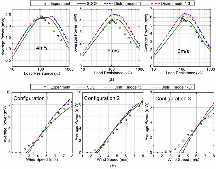
Figure 5. (a) Measured and predicted average power Pave versus load resistance RL for Configuration 1 at U = 4, 5 and 6 m s−1. (b) Measured and predicted average power Pave versus wind speed U for three configurations at the respective optimum RL.
Download figure:
Standard image High-resolution image5. Parametric study using distributed parameter model (first mode)
In this section, a parametric study is presented in order to better understand the electroaeroelastic behavior of the GPEH. The effects of load resistance RL, wind exposure area Stip, mass of the bluff body Mtip, and length of the piezoelectric sheets Lp on the cut-in wind speed as well as the output power level are investigated.
5.1. Effects of the load resistance RL
Figure 6(a) shows the variation of the average output power Pave with the wind speed U for different load resistances RL. Here, Configuration 1 is considered and its properties are shown in tables 1 and 2. It can be seen that the growth rate of Pave is greatly affected by RL. The growth rate of Pave firstly increases with RL until 105 kΩ, then decreases when RL is further increasing. An enlarged view is provided to show this trend more clearly around the threshold of galloping. It is noted that the value of RL which owns the largest growth rate of Pave also gives the largest cut-in wind speed Ucr. The variation of Ucr with RL is presented in figure 6(b). As can be seen from this curve, Ucr increases with RL up to the maximum value then decreases with RL. As for the harvested power level, the largest power is obtained with RL around 105 kΩ for U > 4 m s−1. Features of the optimum RL can be seen from figure 6(c) which displays the variation of Pave with RL at different wind speeds. For U = 2 m s−1, Pave is zero between 20 and 800 kΩ since this speed is lower than the respective Ucr for these RL values (figure 6(b)). When U is slightly larger than Ucr (i.e., U = 3 and 4 m s−1), a shallow valley exists around 105 kΩ. When U continues growing (i.e., U = 5–8 m s−1), there is a peak for Pave between 100 and 120 kΩ, where lies the optimum RL = 105 kΩ. It is worth mentioning that RL for the valley and the peak of Pave overlap with each other, corresponding to that with the largest Ucr. From here onwards, we regard RL as the optimum one if the largest Ucr and power growth rate are achieved in the response of Pave versus U (i.e., the curve for RL = 105 kΩ in figure 6(a)). At the optimum RL, either a valley or a peak appears in the response of Pave versus RL at a specific U.
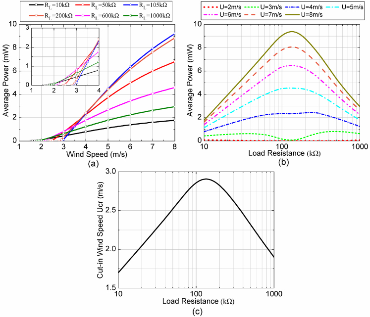
Figure 6. (a) Variation of the average power Pave with the wind speed U for different load resistances. (b) Variation of the average power Pave with the load resistance RL for different wind speeds. (c) Variation of the cut-in wind speed Ucr with the load resistance.
Download figure:
Standard image High-resolution image5.2. Effects of the wind exposure area of the bluff body Stip
Figure 7 shows the effects of the wind exposure area of the bluff body Stip (h × ltip) on the electroaeroelastic behavior of the GPEH. The harvester properties are the same as those listed in tables 1 and 2 (Configuration 1) except the length of the bluff body ltip. Figure 7(a) is obtained with U = 6 m s−1. It is determined that the optimum RL for the various Stip are equal to each other, which is reasonable since the natural frequencies are the same with equal Mtip. The variation of Pave with U at the optimum RL for different Stip is shown in figure 7(b). With increasing Stip, the cut-in wind speed decreases while the harvested power increases, both beneficial for harvesting the wind power. This can be expected since the increasing wind exposure area results in an increase in the aerodynamic force. Moreover, the growth rate of power is not much affected by Stip.
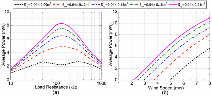
Figure 7. Variation of (a) the average power Pave with the load resistance RL at 6 m s−1 and (b) the average power Pave with the wind speed U at the optimum RL for different wind exposure areas of the bluff body Stip.
Download figure:
Standard image High-resolution image5.3. Effects of the mass of the bluff body Mtip (or the fundamental frequency of the GPEH)
Figure 8 shows the effects of the mass of the bluff body Mtip on the electroaeroelastic behavior of the GPEH. The harvester properties are the same as those listed in tables 1 and 2 (Configuration 1) except Mtip. The most obvious change due to varying Mtip is in the fundamental frequency of the harvester as indicated in the legend. Figure 8(a) shows the variation of Pave with RL for U = 6 m s−1, from which the respective optimum RL can be obtained for each Mtip. It is noted that the optimum RL varies with different Mtip (i.e., different fundamental frequency ω1). With the respective optimum RL, the variation of Pave with U is displayed in figure 8(b). As can be seen from this figure, the cut-in wind speed increases and the harvested power decreases with the increasing Mtip (or the decreasing of ω1). Moreover, the growth rate of the harvested power also decreases with the increasing Mtip. It can summarized that for the GPEH with a specific piezoelectric cantilever, reducing Mtip can achieve a better performance in extracting power from the wind.
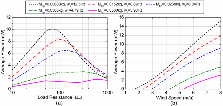
Figure 8. Variation of (a) the average power Pave with the load resistance RL at 6 m s−1 and (b) the average power Pave with the wind speed U at the respective optimum RL for different masses of the bluff body Mtip.
Download figure:
Standard image High-resolution image5.4. Effects of the length of the piezoelectric sheets Lp
Figure 9 shows the effects of the lengths of the piezoelectric sheets Lp on the electroaeroelastic behavior of the GPEH. The harvester properties are the same as those listed in tables 1 and 2 (Configuration 1) except Lp and Cp, since the latter one varies linearly with the former one when other parameters are kept unchanged. The respective optimum RL is determined from figure 9(a), which varies with Lp because of the change in the total stiffness of the composite beam. Figure 9(b) shows the variation of Pave with U at the respective optimum RL. The cut-in wind speed as well as the growth rate of the harvested power increases with the increasing Lp. The largest Lp can extract the highest power at relatively high wind speeds (>12 m s−1). A useful factor to evaluate the performance of the GPEH is the power density which is calculated as power per piezoelectric volume in this paper. Figure 9(c) shows the power density versus the wind speed for different Lp. It is noted that the power density is not monotonically increasing with Lp. At high wind speeds the highest power density is obtained by a medium value of Lp, which is 100 mm among the considered discrete values. A maximum power density of 12.96 mW cm−3 is achieved at 14 m s−1 with Lp = 100 mm. A comparison of the power density with other piezoelectric wind energy harvesters is shown in figure 10. As can be seen from this figure, the present GPEH shows good performance in power density, especially at relatively high wind speeds. The present GPEH is less advantageous at lower wind speeds when compared to the harvesters in [15, 37]. However, the present GPEH has the largest overall range of wind speed for effective power generation with considerable power density. Note that the data for the present GPEH in the figure are not optimized in the aspects of Stip,Mtip, etc.

Figure 9. Variation of (a) the average power Pave with the load resistance RL at 10 m s−1, (b) the average power Pave with the wind speed U at the respective optimum RL and (c) the power density with the wind speed U for different lengths of the piezoelectric sheets Lp.
Download figure:
Standard image High-resolution image
Figure 10. Comparison of the power density with other piezoelectric wind energy harvesters.
Download figure:
Standard image High-resolution image
6. Conclusion
In this paper, a comparison study is presented on the performance of the modeling methods for GPEH, including the SDOF model, and single mode and multi mode Euler–Bernoulli distributed parameter models. A typical GPEH consisting of a piezoelectric cantilever attached to a square-sectioned bluff body is considered. Procedures for these modeling methods are presented, in which the aerodynamic forces are all formulated based on quasi-steady hypothesis. Subsequently, wind tunnel experiments for the fabricated prototypes are conducted to validate and evaluate these models. The results show that all these models can successfully predict the variation of the average power with the load resistance and the wind speed. Quite a small difference is observed between the single mode and multi mode Euler–Bernoulli distributed parameter models. The distributed parameter model has a more rational representation of the aerodynamic force, while the SDOF model gives a better prediction of the cut-in wind speed. In general, the SDOF can predict the electroaeroelastic behavior of a GPEH device accurately enough, with its advantages of simplicity and ease of obtaining the electromechanical coupling term.
The influence of the load resistance, wind exposure area and mass of the bluff body, and the length of the piezoelectric sheets, on the cut-in wind speed as well as the output power level of the GPEH, are investigated with a single mode Euler–Bernoulli distributed parameter model. It is determined that Ucr and the growth rate of Pave increase first with RL to a certain value, then drop with RL. When U is large enough the largest Pave is obtained with the optimum RL, which has the largest Ucr as well. With the corresponding optimum RL, increasing Stip and decreasing Mtip can increase Pave as well as reduce Ucr. For the case of Lp, larger Lp gives larger Ucr and larger growth rate of Pave, yet does not guarantee larger power density (power per piezoelectric volume), which is obtained at a medium Lp. Compared to other piezoelectric wind energy harvesters, our present GPEH gives higher power density at high wind speeds and has the largest range of U with considerable power density. Future work involves improving the performance of the GPEH at low wind speeds.