Abstract
The effects of ambient temperature on the level of harvesting energy from galloping oscillations of a bluff body are investigated. A nonlinear-distributed-parameter model is developed to determine variations in the onset speed of galloping and the level of the harvested power when the ambient temperature is varied. The considered harvester consists of a bimorph piezoelectric cantilever beam with a prismatic-structure tip mass. A modal analysis is performed to derive the exact mode shapes and natural frequencies of the beam–structure system and their dependence on temperature variations. The quasi-steady representation is used to model the aerodynamic loads. The linear analysis shows that the temperature and the electrical load resistance affect the onset speed of galloping significantly. The nonlinear analysis shows that temperature variation affects the level of the harvested power.
Export citation and abstract BibTeX RIS
1. Introduction
Piezoelectric transduction-based energy harvesting systems have received significant attention as viable long-term power sources that can be effectively placed in small volumes and used to harvest energy over a wide range of frequencies. These harvesters have been proposed to operate self-powered devices including microelectromechanical systems or actuators [1–3], health monitoring, and wireless sensors [4, 5], or to replace small batteries that have a finite life span or would require hard and expensive maintenance [6–8]. However, several structural and environmental factors can affect the performance of these harvesters. One of these factors that can change the response of a piezoelectric energy harvester is the ambient temperature. This is due to the fact that temperature variations affect the properties of piezoelectric materials [9–12]. Rhimi and Lajnef [13] studied the effects of the temperature on the response of a piezoelectric energy harvester subjected to direct excitations. They determined that variations in the temperature of a specific piezoelectric material (PZT-5H) affected the frequency of the harvester and, consequently, the level of the harvested power.
There has also been recent interest in the concept of harvesting energy from aeroelastic or flow-induced vibrations [14–21]. In these studies, one or two piezoceramic layers bonded by electrodes that generate an alternating voltage output are used to convert flow-induced vibrations to electrical power. Another aeroelastic phenomenon that has shown promise for harvesting energy is the galloping of prismatic structures. Sirohi and Mahadik [22] proposed harvesting energy from transverse galloping of a structure that had an equilateral triangle section. Surface-bonded piezoelectric sheets attached to two beams connected to the structure were used to harvest power. Their device generated more than 50 mW at a wind speed of 11.6 mph, a power level that is sufficient to supply most of the commercially available wireless sensors. Abdelkefi et al [23] derived a nonlinear distributed-parameter model for galloping-based piezoaeroelastic energy harvesters. They validated their numerical results with the experimental measurements of Sirohi and Mahadik [22]. Abdelkefi et al [24, 25] investigated the effects of the Reynolds number and section geometry on the level of harvested power. Their results showed the combined effects of the electrical (load resistance) and mechanical (damping and frequency) components on the harvester's response. Noting that the ambient temperature impacts the piezoelectric material properties, one would certainly expect it to add to the combination of parameters that affect the harvester's response.
In this work, the impact of the temperature on the performance of a galloping-based piezoaeroelastic energy harvester is investigated. To this end, we consider a bimorph piezoelectric (PZT-5H) cantilever beam with a prismatic-structure tip mass. We develop a nonlinear distributed-parameter model that is capable of predicting the level of harvested power that can be generated from galloping oscillations for different temperatures, wind speeds, and load resistances. The developed electromechanical model which takes into account the impact of the temperature on the system's response is discussed in section 2. The quasi-steady approximation is used to model the aerodynamic loads. The background and justification for using this model are discussed in section 3. In section 4, linear and nonlinear analyses of the system are performed to investigate the effects of the temperature and electrical load resistance on the onset of galloping, harvested power, voltage output, and tip displacement amplitude. A summary and conclusions are presented in section 5.
2. System modeling and reduced-order model
2.1. Governing equations
The energy harvester shown in figure 1 consists of a piezoelectric bimorph cantilever beam with a prismatic structure attached to its free end. This structure undergoes galloping in the transverse direction when subjected to an incoming flow. The cantilever beam is composed of aluminum and two piezoelectric layers (PZT-5H). The piezoelectric sheets are bonded by two in-plane electrodes of negligible thickness connected in parallel with opposite polarity to a load resistance R. The geometric and material properties of the harvester are presented in table 1.

Figure 1. A schematic of the piezoaeroelastic energy harvester.
Download figure:
Standard imageTable 1. The physical and geometric properties of the cantilever beam and the tip body.
| Es | Aluminum Young's modulus (GN m−2) | 70 |
| ρs | Aluminum density (kg m−3) | 2700 |
| ρp | PZT-5H density (kg m−3) | 7900 |
| L | Length of the beam (mm) | 90 |
| b1 | Width of the aluminum layer (mm) | 38 |
| b2 | Width of the piezoelectric layer (mm) | 36.2 |
| hs | Aluminum layer thickness (mm) | 0.635 |
| hp | Piezoelectric layer thickness (mm) | 0.267 |
| Mt | Tip mass (g) | 65 |
| Lstruc | Length of the tip body (mm) | 235 |
| bstruc | Width of the tip body (mm) | 30 |
The Euler–Bernoulli beam assumptions are used to model the multilayered cantilever beam. Based on these assumptions, the transverse vibration, v(x;t), of the cantilever beam is described by
where δ(x) is the Dirac delta function, Ftip and Mtip are, respectively, the galloping aerodynamic force and moment at the tip of the beam that are caused by the oscillation of the structure, L is the length of the beam, ca is the viscous air damping coefficient, m is the mass of the beam per unit length, and M(x;t) is the internal moment. This moment is composed of three components. The first is the resistance to bending and is given by  . The second is due to the strain rate damping effect and is represented by
  . The third component is the contribution of the piezoelectric sheets which are connected in parallel. This contribution is represented by (H(x) − H(x − L))ϑpV(t) where H(x) is the Heaviside step function, V(t) is the generated voltage, and ϑp is the piezoelectric coupling term [26]. This term is given by

where e31 is the piezoelectric stress coefficient, b2 is the width of the piezoelectric layer and hs and hp are the thicknesses of the aluminum and piezoelectric layers, respectively.
Substituting for the moment M(x;t) its three components in equation (1), the equation of motion of the electromechanical system is rewritten as
In this equation, the stiffness EI and mass of the beam per unit length m are given by ![$E I=\frac{1}{1 2}{b}_{1}{E}_{\mathrm{s}}{h}_{\mathrm{s}}^{3}+\frac{2}{3}{b}_{2}{E}_{\mathrm{p}}[({h}_{\mathrm{p}}+\frac{{h}_{\mathrm{s}}}{2})^{3}-\frac{{h}_{\mathrm{s}}^{3}}{8}]$](https://content.cld.iop.org/journals/0964-1726/22/5/055026/revision1/sms459449ieqn70.gif) and m = b1ρshs + 2b2ρphp where Es and Ep are the Young's moduli of the aluminum and piezoelectric layers, respectively, and ρs and ρp are the respective densities of these layers.
and m = b1ρshs + 2b2ρphp where Es and Ep are the Young's moduli of the aluminum and piezoelectric layers, respectively, and ρs and ρp are the respective densities of these layers.
To complete the problem formulation, we relate the mechanical and electrical variables by using the Gauss law [27]

where D is the electric displacement vector and n is the normal vector to the plane of the beam. The electric displacement component D2 is given by the following relation [26]:

where ε11 is the axial strain component in the aluminum and piezoelectric layers and is given by  is the permittivity component at constant strain. Substituting (5) into (4), we obtain the equation governing the strain–voltage relation,
2.2. Eigenvalue problem analysis
To perform the linear and nonlinear analyses, we first discretize the system using the Galerkin procedure which requires the exact mode shapes of the structure. To determine the mode shapes of the considered system, we drop the damping, forcing, and polarization from equation (3), and let v(x,t) = ϕ(x)eiωt. The resulting eigenvalue problem is given by

with the following boundary conditions:


where It is the rotary inertia of the tip structure Mt and Lc is half of the length of the tip mass. The general expression of the mode shapes is written as

where β and ω are related by  .
.
To obtain the relation between the different coefficients in (11), we normalize the eigenfunctions and use the following orthogonality conditions:

where s and r are used to represent the vibration modes and δrs is the Kronecker delta, defined as unity when s is equal to r and zero otherwise.
Using the Galerkin discretization, we express the transverse displacement, v(x,t), in the following form:
where qi(t) are the modal coordinates and ϕi(x) are the mode shapes of the cantilever beam with the prismatic tip structure. Substituting equation (14) into equations (3) and (6) and considering the first mode only, we obtain the following coupled equations of motions:


where ξ is the mechanical damping coefficient, f(t) is the galloping force of the first mode which is expressed as f(t) = ϕ(L)Ftip + ϕ'(L)Mtip,ω is the fundamental natural frequency of the structure, and the coefficients θp and Cp are the piezoelectric coupling term and the capacitance of the harvester which are given by θp = ϕ'(L)ϑp and  .
.
2.3. Temperature effects on the piezoelectric material (PZT-5H) properties
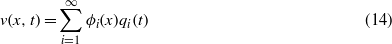
Inspecting the governing equations of the harvester (equations (3) and (6)), we note that these equations depend on the properties of the piezoelectric material (Ep,e31, and  ). It has been demonstrated in the literature [10] that the temperature can significantly affect the properties of the piezoelectric material. The plotted curves in figure 2 show the effects of the temperature on the piezoelectric and dielectric constants and Young's modulus of the PZT-5H. The red points represent the values measured by Hooker [10] and the solid lines are fitted polynomials to be considered in our subsequent analysis. Figure 2(a) shows that the temperature affects the piezoelectric constant d31 = e31/Ep significantly. In fact, an increase of about 200% in the piezoelectric constant is obtained when the temperature is varied from −70 to 120 °C. For the dielectric constant,
  , where ε0 is the permittivity of free space and
  is the permittivity component at constant stress, an increase in the operating temperature from −70 to 120 °C causes a significant increase of about 300%, as shown in figure 2(b). The variation of the PZT-5H Young's modulus as a function of the temperature is plotted in figure 2(c). A decrease of about 30% is obtained when the temperature is increased from −20 to 50 °C. Clearly, the properties of the PZT-5H are strong functions of the operating temperature.
Figure 2. Variations of the PZT-5H properties as a function of the temperature based on the experimental data of Hooker [10] (red points): (a) piezoelectric constant, (b) dielectric constant, and (c) Young's modulus. The solid lines represent the considered fitting in the numerical analysis.
Download figure:
Standard imageNoting that the structural natural frequency of the harvester, ω, depends on the Young's modulus through the relation  , where
 ![$E I=\frac{1}{1 2}{b}_{1}{E}_{\mathrm{s}}{h}_{\mathrm{s}}^{3}+\frac{2}{3}{b}_{2}{E}_{\mathrm{p}}[({h}_{\mathrm{p}}+\frac{{h}_{\mathrm{s}}}{2})^{3}-\frac{{h}_{\mathrm{s}}^{3}}{8}]$](https://content.cld.iop.org/journals/0964-1726/22/5/055026/revision1/sms459449ieqn124.gif) , and that varying the temperatures causes variations in the value of Ep, it is clear that the structural natural frequency depends on the temperature. Figure 3(a) shows the variation of the structural natural frequency as a function of the temperature. The plots show that increasing the temperature from −20 to 50 °C causes the natural frequency to decrease by about 15%. This is expected because the Young's modulus, Ep, is reduced when the temperature is increased, as shown in figure 2(c). The variations of the piezoelectric constant and dielectric constant, as shown in figures 2(a) and (b), result in variations in the capacitance, Cp, and piezoelectric coupling, θp. In fact, the capacitance is directly related to
, and that varying the temperatures causes variations in the value of Ep, it is clear that the structural natural frequency depends on the temperature. Figure 3(a) shows the variation of the structural natural frequency as a function of the temperature. The plots show that increasing the temperature from −20 to 50 °C causes the natural frequency to decrease by about 15%. This is expected because the Young's modulus, Ep, is reduced when the temperature is increased, as shown in figure 2(c). The variations of the piezoelectric constant and dielectric constant, as shown in figures 2(a) and (b), result in variations in the capacitance, Cp, and piezoelectric coupling, θp. In fact, the capacitance is directly related to  by the relation
  and the piezoelectric coupling coefficient is expressed as a function of e31 by θp =− e31b2(hp + hs)ϕ'(L). The variations of the capacitance and piezoelectric coupling coefficients as functions of the temperature are plotted in figures 3(b) and (c), respectively. The plot in figure 3(b) shows that increasing the temperature from −20 to 50 °C causes the capacitance of the piezoelectric material to increase by about 78%. This is due to the increase in the permittivity at constant strain
  . On the other hand, there is an optimum value of the temperature at which the piezoelectric coupling is maximized, as shown in figure 3(c). This coupling increases when the temperature is increased from −20 °C to almost 0 °C and then decreases as the temperature is raised from 0 to 50 °C. Because of the significant impact of the temperature on the piezoelectric coupling, the capacitance of the piezoelectric material, and the natural frequency of the harvester, one would expect the harvester's response to be strongly dependent on the operating temperature.

Figure 3. Variations of the (a) structural natural frequency, (b) capacitance of the piezoelectric material, and (c) piezoelectric coupling as functions of the temperature.
Download figure:
Standard image3. Aerodynamic load representation
The aerodynamic loads are modeled by using the quasi-steady approximation [28, 29]. In fact, in the transverse galloping phenomenon, the characteristic time scale of the oscillations, which is approximately equal to  , is, in general, much larger than the characteristic time scale of the flow motion, which is of the order of
  where bstruc is the width of the bluff body at the tip. Because the length of the tip mass is large, there are two different components in the aerodynamic loads, namely the galloping force and the galloping moment. These loads are directly related to the lift and drag forces FL and FD by
where Lstruc is the length of the tip structure, s is the length coordinate along the tip structure, and the lift force FL and the drag force FD per unit length are given by

where ρair is the density of air, bstruc is the width of the tip structure, and U is the incoming wind speed. Here, CL and CD are, respectively, the lift and drag coefficients. These aerodynamic coefficients depend on the angle of attack, α, as well as the Reynolds number. For the considered system, the angle of attack is expressed as  .
.
To simplify the analysis, we consider the total aerodynamic force per unit length, Fy, applied to the prismatic structure in the direction normal to the incoming flow. This total force is directly related to the lift and drag forces and is given by
where Cy is the total aerodynamic force coefficient in the direction normal to the incoming flow.
Following Barrero-Gil et al [29], the total aerodynamic force coefficient can be expressed by a polynomial function of tan(α) in the form

where a1 and a3 are empirical coefficients obtained by polynomial fitting of Cy versus tan(α). The Den Hartog stability criterion [30] states that a section of a prismatic structure on a flexible support is susceptible to galloping when the linear coefficient a1 is positive. In fact, galloping is a self-excited response, which is initiated when the damping of the system changes from positive to negative. The nonlinear coefficient a3 is always negative because Cy always has a maximum value, which decreases as a function of the angle of attack. Both the linear and nonlinear coefficients depend on the geometry of the cross-section and the aspect ratio of the prismatic structure. To investigate the effects of the temperature on the onset speed of galloping, we consider two different isosceles cross-section geometries, namely isosceles triangles with δ = 30° and 53°. Barrero-Gil et al [29] give empirical values of both of a1 and a3, as presented in table 2. These values are used in the rest of the analysis. Based on the above derivation and assumptions, the aerodynamic loads are expressed as
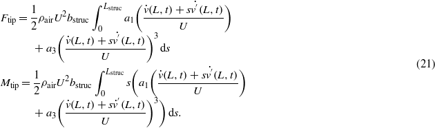
Table 2. Estimates of the linear and nonlinear coefficients for different cross-section geometries.
| Cross-section | a1 | a3 |
|---|---|---|
| Isosceles triangle (δ = 30°) [31, 29] | 2.9 | −6.2 |
| Isosceles triangle (δ = 53°) [32, 29] | 1.9 | −6.7 |
Using the Galerkin discretization in equation (21), the combined term for the aerodynamic force and moment is rewritten as

where k1 and k3 are given by
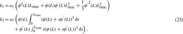
It was demonstrated in section 2.2 that the eigenfunctions of the system are independent of the temperature variations and that only the natural frequency is changed. Consequently, the global galloping force is independent of the temperature.
4. Results and discussion
To analyze the representative model, the governing equations of the galloping-based piezoaeroelastic energy harvester are rewritten using the following state variables:
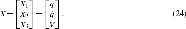
The equations of motion are then written as

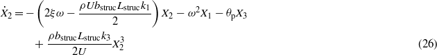

These equations have the form

where
and C(X,X,X) is a cubic vector of the state variables which is given by ![${\mathbf{C}}^{T}=[\begin{array}{@{}c@{}} \displaystyle 0,\frac{\rho {b}_{\mathrm{struc}}{L}_{\mathrm{struc}}{k}_{3}}{2 U}{X}_{2}^{3},0 \end{array}]$](https://content.cld.iop.org/journals/0964-1726/22/5/055026/revision1/sms459449ieqn186.gif) .
.
4.1. Linear analysis: temperature effects on the onset speed of galloping
The effects of the temperature and electrical load resistance on the onset speed of galloping are determined from a linear analysis. The matrix B includes all parameters that affect the linear part of the system. In this matrix, three variables are dependent on the temperature. These are the structural natural frequency, ω, the capacitance of the piezoelectric material, Cp, and the piezoelectric coupling, θp. B(U) has a set of three eigenvalues λi, i = 1,2,3, which vary with the temperature. The first two eigenvalues are similar to those of a pure galloping problem in the absence of the piezoelectricity effect. The third eigenvalue, λ3, is a result of the electromechanical coupling and is always real and negative, as in the case of piezoelectric systems subjected to base or aeroelastic excitations [33–35, 17]. The first two eigenvalues are complex conjugates ( ). The real part of these eigenvalues represents the electromechanical damping coefficient and the positive imaginary part corresponds to the global frequency of the coupled system. Because λ3 is always real and negative, the stability of the trivial solution depends only on the real part of the first two eigenvalues. The solution of the linear part is asymptotically stable if the real part of λ1 is negative. On the other hand, if the real part of λ1 is positive, the solution of the linearized system is unstable. The speed, Ug, for which the real part of λ1 is zero corresponds to the onset of instability or galloping. Because Real (dλ1/dU) is nonzero at Ug, the instability or bifurcation is a Hopf bifurcation.
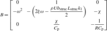
Figures 4(a) and (b) show the variation of the onset speed of galloping with the electrical load resistance for the two considered cross-section geometries and for different values of the temperature when using the physical and geometric properties described in table 1. The plots show that the load resistance affects the onset speed of galloping significantly for both considered configurations and for different temperature values. In the lower range (R < 103 Ω) and for different values of the temperature, the rate of variation is negligible. This rate increases significantly over a middle range of resistance values and yields a peak for the onset speed when the electrical load resistance is between 104 and 105 Ω for all considered temperature values. At higher load resistances (R > 107 Ω), the onset speed of galloping decreases again to values that are close to those obtained in the low-resistance range for all considered temperatures. The minimum values for the onset speed of galloping in the low- and high-resistance ranges correspond to the minimum values of the coupled electromechanical damping over the same range of load resistances. Furthermore, the plots show that the temperature affects the onset speed of galloping strongly in the middle range of the resistance values (i.e. between 104 and 105 Ω). As the temperature is increased, the onset speed of galloping is decreased. This is expected because this value is dependent on the structural natural frequency, the capacitance of the piezoelectric material, and the piezoelectric coupling; these vary with the temperature and their variations affect the coupled electromechanical damping. The plots also show that the speed at the onset of instability strongly depends on the geometry of the cross-section. Indeed, the isosceles triangle with δ = 30° has a lower speed for any load resistance when compared to the isosceles triangle with the δ = 53° cross-section. On inspecting the relation between the onset speed of galloping and the linear system parameters, it is noted that the larger the value of the linear coefficient a1 is, the smaller the onset speed is.
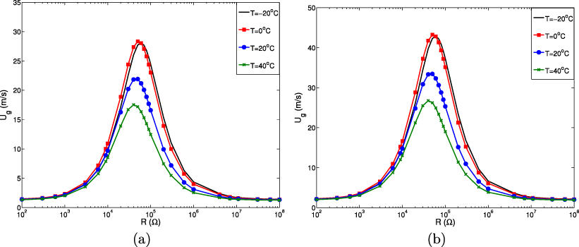
Figure 4. Variation of the onset speed of galloping, Ug, as a function of the load resistance for different values of the temperature and for different cross-section geometries: (a) isosceles triangle with δ = 30° and (b) isosceles triangle with δ = 53°.
Download figure:
Standard imageTo further investigate the effects of the temperature on the onset speed of galloping, we plot in figures 5(a) and (b) the variation of the onset speed of galloping as a function of the temperature for different values of the electrical load resistance and for the two cross-section geometries. For R = 103 and 107 Ω, the impact of the temperature on the onset speed of galloping is very negligible. For R = 104 and 106 Ω, varying the temperature affects the onset speed of galloping significantly. In fact, at higher temperatures, the onset speed of galloping decreases when the temperature is increased. For R = 105 Ω, the onset speed of galloping changes significantly when the temperature is varied. At low temperature values, the onset speed is very high, with a maximum value near T ≈− 15 °C. At higher temperature values, it decreases drastically. This significant variation in the onset speed of galloping when varying the temperature is due to the dependence of the piezoelectric properties on the temperature and their effects on the coupled electromechanical damping. As we note the same tendency for the two cross-section geometries considered, we will consider only the isosceles triangle with δ = 30° in the rest of this work.

Figure 5. Variation of the onset speed of galloping, Ug, as a function of the temperature for different load resistances and for different cross-section geometries: (a) isosceles triangle with δ = 30° and (b) isosceles triangle with δ = 53°.
Download figure:
Standard image4.2. Nonlinear analysis: temperature impact on the performance of the harvester
To investigate the impact of the temperature, electrical load resistance, and wind speed on the performance of the harvester, we perform a full nonlinear analysis of the governing equations. The bifurcation diagrams of the tip displacement of the bluff body for different temperatures and when the electrical load resistance is set equal to 103 Ω,104 Ω,105 Ω, and 106 Ω are shown in figures 6(a)–(d), respectively. On inspecting these curves, we find that the load resistance affects the onset speed of galloping strongly, as demonstrated by the linear analysis performed in section 4.1. The onset speed of galloping is always lower at higher temperature values for all considered load resistances. The impact of the temperature on the onset speed is very negligible for R = 103 Ω, as shown in figure 6(a). For R = 105 Ω, the onset speed changes significantly when the temperature value is varied, as shown in figure 6(c). The displacement values are zero for T =− 20 and 0 °C for wind speeds less than 20 m s−1. This is expected because the onset speeds of galloping for these two temperatures are larger than 20 m s−1 for a load resistance of 105 Ω, as shown in figure 5(a). Additionally, the maximum displacement values are observed when T = 40 °C for all considered load resistances. This is explained by the low values of the electromechanical damping at this temperature.
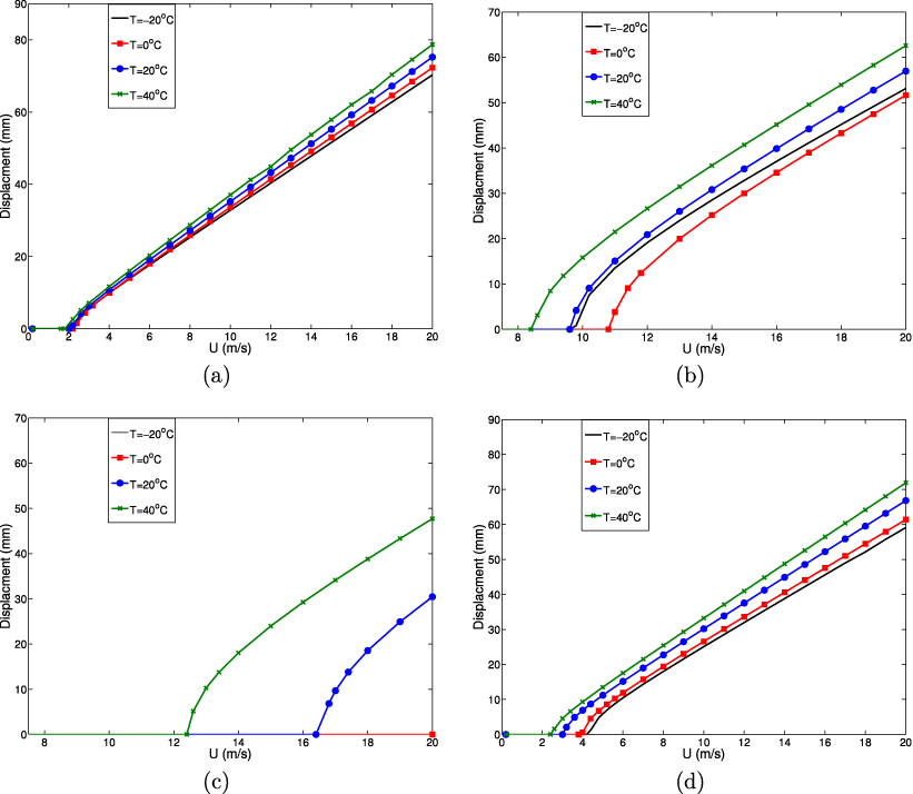
Figure 6. Bifurcation diagrams of the tip displacement for different values of the temperature and electrical load resistance: (a) R = 103 Ω, (b) R = 104 Ω, (c) R = 105 Ω, and (d) R = 106 Ω.
Download figure:
Standard imageFigure 7 shows the impact of the temperature on the voltage output for different values of the load resistance when varying the wind speed. For R = 103 Ω, a higher value of the generated voltage is obtained when the temperature is 0 °C, as shown in figure 7(a). Furthermore, there is an intersection point between the different curves of the generated voltage when varying the temperature for R = 103,104, and 106 Ω, as shown in figures 7(a), (b), and (d). The wind speed corresponding to this intersection point is closer to the onset speed of galloping when the impact of the temperature on the onset speed is less pronounced. For R = 103 Ω, the intersection point is very close to the onset of instability. For R = 104 Ω, the intersection point is significantly higher than the onset speed. Beyond this intersection point, the generated voltage, for the cases where the onset speed of galloping is relatively larger, becomes more important. This result is very clear in figures 7(a) and (d).
Figure 7. Bifurcation diagrams of the generated voltage for different values of the temperature and electrical load resistance: (a) R = 103 Ω, (b) R = 104 Ω, (c) R = 105 Ω, and (d) R = 106 Ω.
Download figure:
Standard imageThe plotted curves in figure 8 show the bifurcation diagrams of the harvested power for different temperatures and load resistances. The lowest values of the harvested power are obtained at T = 40°C for R = 103 and 106 Ω, as shown in figures 8(a) and (d), respectively. It is important to note that these minimum values in the harvested power are associated with maximum values of the tip displacement, as shown in figures 6(a) and (d), The highest values of harvested power are obtained in cases where the onset speeds of galloping are higher. These maximum values of the harvested power are associated with minimum values of the tip displacement, as shown in figures 6(a) and (d), for R = 104 and 105 Ω. All of these results show the significant impact of the temperature on the response of the harvester.
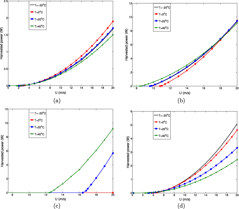
Figure 8. Bifurcation diagrams of the harvested power for different values of the temperature and electrical load resistance: (a) R = 103 Ω, (b) R = 104 Ω, (c) R = 105 Ω, and (d) R = 106 Ω.
Download figure:
Standard imageTo further elucidate the effects of the temperature on the system's outputs, we plot in figures 9 and 10 the variation of the tip displacement, generated voltage, and harvested power as functions of the temperature for different load resistances and for two distinct values of the wind speed, namely 5 and 15 m s−1. For U = 5 m s−1, figures 9(a)–(c) show that no power can be generated for electrical load resistance values of 104 or 105 Ω. For R = 103 Ω and U = 5 m s−1, increase of the temperature is accompanied by a slight increase in the tip displacement, as shown in figure 9(a), and a slight decrease in the harvested power, as shown in figure 9(c). For R = 106 Ω and U = 5 m s−1, the tip displacement increases as the temperature is increased. This is explained by the low electromechanical damping terms at these temperatures. Figure 9(c) shows that increasing the temperature also causes an increase in the harvested power level.

Figure 9. Variation of the (a) tip displacement, (b) generated voltage, and (c) harvested power as a function of the temperature for different load resistances and when U = 5 m s−1.
Download figure:
Standard image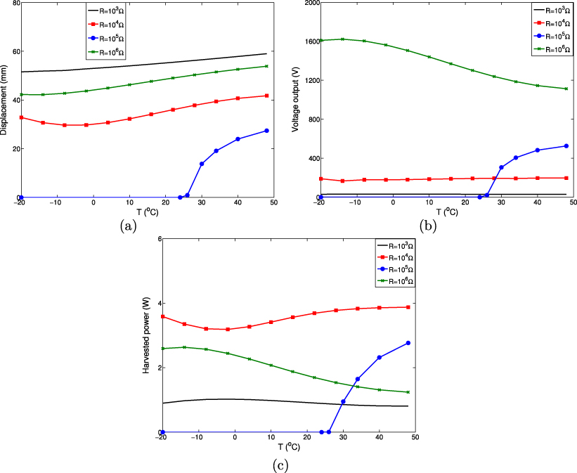
Figure 10. Variation of the (a) tip displacement, (b) generated voltage, and (c) harvested power as a function of the temperature for different load resistances and when U = 15 m s−1.
Download figure:
Standard imageAt U = 15 m s−1, figure 10(a) shows that increase of the temperature is accompanied by an increase in the displacement for the considered load resistances. This is due to the low electromechanical damping at the high temperature values. On the other hand, the generated voltage and harvested power show different tendencies when using different load resistances. Because the intersection wind speed values when the load resistances are set equal to 103 and 106 Ω are smaller than this wind speed (15 m s−1), the variations of the generated voltage and harvested power with the temperature, as shown in figures 10(b) and (c), have similar tendencies to the variation of the onset speed of galloping with the temperature. These results show that maximum levels of harvested power are accompanied by minimum values of tip displacement when varying the temperature, and vice versa. For a load resistance of 104 Ω, there is a minimum value in the tip displacement when the temperature is between −5 and 0 °C, as shown in figure 10(a). This range of temperature corresponds to a higher onset speed of galloping, as shown in figure 5(a). Because the intersection wind speed value is larger than the considered speed, the curves of the tip displacement, generated voltage, and harvested power have the same tendency when varying the temperature, as shown in figures 10(a)–(c). For R = 105 Ω, the harvester does not produce any power at temperatures lower than 26 °C. This is expected because the onset speed of galloping is larger than 15 m s−1 in this range of temperatures, as shown in figure 5(a). In addition, increase of the temperature is associated with an increase in all of the system's outputs.
To further investigate the effects of the electrical load resistance on the system outputs for different values of the temperature, we present in figures 11, 12 and 13 the variation of the tip displacement, generated voltage, and harvested power, respectively, with the electrical load resistance for four values of the temperature and two distinct wind speeds, namely U = 5 m s−1 and U = 15 m s−1. On inspecting figures 11(a), 12(a), and 13(a), it is noted that for U = 5 m s−1 there is a range of load resistance where no oscillations (zero-tip displacement) are observed. This range of load resistance depends on the temperature. This is expected because the onset speed of galloping in this region of load resistance is larger than U = 5 m s−1. These zero-displacement values can be explained by the maximum value of the electromechanical damping in this region of electrical load resistance. When the wind speed is increased to U = 15 m s−1, as shown in figures 11(b), 12(b), and 13(b), we find that the range of zero-tip displacement is decreased progressively for all considered temperature values. For all considered temperature values, for low (R < 103 Ω) and high (R > 107 Ω) load resistance values, the variation of the displacement with the electrical load resistance is negligible for both wind speeds, as shown in figures 11(a) and (b).
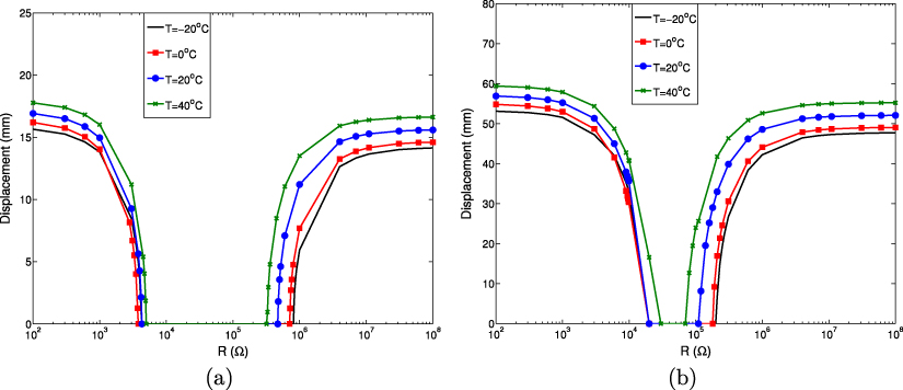
Figure 11. Variation of the tip displacement as a function of the electrical load resistance when (a) U = 5 m s−1 and (b) U = 15 m s−1 and for different temperature values.
Download figure:
Standard image
Figure 12. Variation of the generated voltage as a function of the electrical load resistance when (a) U = 5 m s−1 and (b) U = 15 m s−1 and for different temperature values.
Download figure:
Standard image
Figure 13. Variation of the harvested power as a function of the electrical load resistance when (a) U = 5 m s−1 and (b) U = 15 m s−1 and for different temperature values.
Download figure:
Standard imageFigures 12(a) and (b) show the variation of the generated voltage with the load resistance for different temperature values. It is noted that, for low and high values of the load resistance, increase of the electrical load resistance is associated with an increase in the generated voltage for all considered temperature values and for both considered wind speeds. Moreover, the generated voltage stabilizes for a specific value of the electrical load resistance, which is around 107 Ω when U = 5 m s−1 and 106 Ω when U = 15 m s−1. As mentioned above, for a specific range of load resistance, only at high temperature (T = 40 °C) can the system harvest energy. Furthermore, the level of generated voltage is higher at lower temperatures.
The plots in figure 13 show the variation of the harvested power with the load resistance for different values of the temperature and for two distinct wind speeds. The plots show that there are optimum values of the load resistance for which more energy can be harvested and these optimum values depend on the temperature and the wind speed considered. Similarly to the variation of the tip displacement and generated voltage with the load resistance, the harvested power is almost zero over a specific range of load resistance that is temperature-dependent. Moreover, the region of load resistance over which the harvested power is maximum matches the region of load resistance over which the displacement is minimum, and vice versa, for all considered temperature values and for both wind speeds. These results show that at higher temperature values, energy harvesting can be performed at lower wind speeds. In the low-temperature range, the level of harvested power can be maximized but this will be achieved only at higher wind speeds.
5. Conclusions
The impact of the temperature on the properties of PZT-5H piezoelectric material and on the onset speed of galloping and the level of harvested power of a galloping-based piezoaeroelastic energy harvester was investigated. The harvester consisted of a bimorph piezoelectric cantilever beam with a prismatic-structure tip mass. A nonlinear-distributed-parameter model was used to perform the analysis. The quasi-steady approximation was used to model the galloping force and moment. Linear and nonlinear analyses were performed to investigate the effects of the temperature and electrical load resistance on the onset of instability and the system's response. The results showed that the system's response is strongly affected by temperature variation. It was determined that the effects of varying the operating temperature are more significant at specific load resistances and wind speeds. At higher temperature values, energy can be harvested at lower wind speeds and for different load resistances. On the other hand, at relatively higher wind speeds, more energy can be generated at lower temperatures. The maximum levels of harvested power are always associated with minimum displacements. These results show a complex relation between the harvested power and tip displacement on one hand and the wind speed, load resistance, and temperature on the other hand. This complex relation necessitates the development of representative models and coupled analysis as performed here.