
Abstract
We present an energy harvester for environments that rotate through the Earth's gravitational field. Example applications include shafts connected to motors, axles, propellers, fans, and wheels or tires. Our approach uses the unique dynamics of an offset pendulum along with a nonlinear bistable restoring spring to improve the operational bandwidth of the system. Depending on the speed of the rotating environment, the system can act as a bistable oscillator, monostable stiffening oscillator, or linear oscillator. We apply our approach to a tire pressure monitoring system mounted on a car rim. Simulation and experimental test results show that the prototype generator is capable of directly powering an RF transmission every 60 s or less over a speed range of 10 to 155 kph.
Export citation and abstract BibTeX RIS
1. Introduction
The ability to harvest or scavenge energy from a wireless sensor's operating environment can facilitate many sensing applications in which regular replacement or recharging of batteries is either not possible or expensive [1, 2]. Many potential energy sources have been studied, including vibrations [3], temperature gradients [4], and human motion [5]. Harvesting energy from a rotating environment (i.e., rotating machinery, wheels, shafts, propellers, etc) can be considered a subset of vibration energy harvesting, but has unique dynamics that benefit from different solutions. A tire pressure monitoring system (TPMS) is a good example of an application in which energy harvesting from a rotating environment is beneficial. TPMS modules are mounted on the car rim, which are attached to inside of the valve stem (see figure 1). They periodically measure tire pressure and send that information via wireless transmission to a receiver located near the center of the car. TPMS have been standard on all cars sold in the United States since 2006 [6]. Current systems are battery powered. The battery is not replaceable and, as the TPMS is attached to the wheel rather than the tire, it is intended to last the lifetime of the wheel, which is about 10 years.
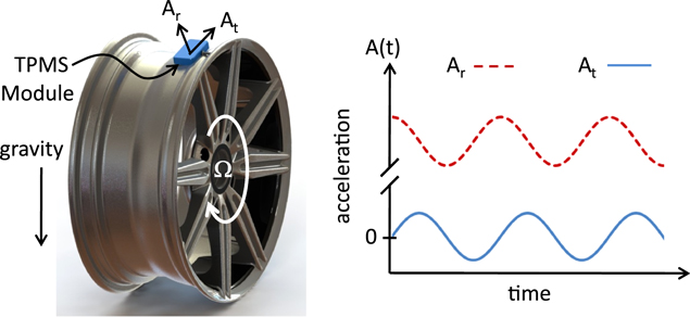
Figure 1. Illustration of TPMS module mounted to a rim. Directions of tangential (At) and radial (Ar) acceleration shown with representative time traces for these two signals.
Download figure:
Standard image High-resolution imageThe TPMS is subjected to a ±1 G excitation at the rolling frequency as the wheel rotates through the Earth's gravitational field (see figure 1). Additionally, higher frequency vibrations are present, although most vibrational energy occurs at the rolling frequency [7]. Therefore, a vibration-powered system would seem to be logical and beneficial to improve the lifetime of the system. A vibration energy harvester for a rim-mounted TPMS must fit within the current size and weight limitations of standard modules. Furthermore, unless a rechargeable battery or super-capacitor is allowed, it must support frequent radio transmissions at both very low and very high speeds. In our experience, the low-speed operation was critical, as rechargeable batteries or super-capacitors were disallowed because of reliability and cost concerns.
There have been prior attempts to develop and commercialize vibration energy harvesters for TPMS. Perhaps most significantly, a system was developed and commercialized in the 1990s [8]. Although this system was a successful commercial product, it would not meet current requirements imposed by car manufacturers. Specifically, the system was too heavy to be safely attached to the inside of a valve stem (the system was attached using a steel band around the rim), too tall to meet the requirements of present day low-profile tires, and would not operate at very low speeds. Some recent work on harvesters for TPMS has focused on potential future tire-mounted systems [9, 10] rather than rim-mounted systems. Other work that focuses on rim-mounted systems [11–13] ignores the power generation at very slow speeds. Manla et al [14] proposed a system that appears similar to the architecture we propose; however, it is actually quite different in the details of operation and system dynamics. Additionally, like the commercialized system of the 1990s, it would be too tall to fit within current TPMS modules. We have previously proposed our harvesting architecture [15, 16]; however, this paper represents the first full description of its operation and unique dynamics.
Most vibration energy harvesting systems operate effectively only at resonance. Thus, for both linear and rotational systems, the narrow operating bandwidth can be a chief limitation. The following three main approaches to improving the bandwidth are the subjects of current research efforts: tuning the resonance frequency of the harvester during operation [17, 18], implementing multimode oscillators [19], and employing nonlinear oscillators to widen the bandwidth [20]. These methods are equally applicable to rotational systems. For example, Gu and Livermore [21] used the dynamics of an offset pendulum to increase the harvester's bandwidth for rotational systems.
In this study, we present the analysis, implementation, and test results for an approach for harvesting energy from a rotating environment. Although we specifically apply our design to the TPMS application, it is applicable to any rotating environment in which the axis of rotation is more or less parallel to the Earth's surface (i.e., horizontal). Like Gu and Livermore [21], our approach takes advantage of the unique features of the dynamics of an offset pendulum to create an inherently broad frequency response. In addition, it contains many unique features that enable efficient power harvesting under the realistic constraints of a TPMS and many rotational systems in which the harvester must be small compared to the rotation radius. Finally, our system incorporates a nonlinear oscillatory motion to further enhance the bandwidth.
The remainder of this paper is organized as follows. First, we present the essence of the dynamics of an offset pendulum rotating through a gravitational field. Then, we discuss the details of the prototype design. This will lead to more detailed modeling and analysis of the dynamics. Finally, we present and discuss the experimental results from both the laboratory and road tests.
2. Offset pendulum dynamics
Figure 2 shows an offset pendulum system mounted on a rotating cylinder or wheel. If the angle (θ) is small, the centripetal acceleration acts like a linear spring, bringing the proof mass back to the center (θ = 0). This effect is illustrated in figure 3.

Figure 2. Illustration of an eccentrically mounted pendulum on rotating wheel or shaft. The centripetal acceleration on the proof mass acts like a linear spring as long as θ is small.
Download figure:
Standard image High-resolution image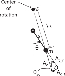
Figure 3. Effect centripetal acceleration on the proof mass. The centripetal acceleration (Ac) creates a restoring force in the tangential direction, which is proportional to the angular displacement (θ). (Because the acceleration from gravity is small compared to Ac, it is ignored in this figure).
Download figure:
Standard image High-resolution imageEquations (1)–(5) show the derivation of the effective torsional stiffness on the proof mass (kθ ) and its natural oscillation frequency (ωn ). The derivation uses the small angle approximation. Specifically, it is assumed that sin(θ) = θ and L3 = L1 + L2. As indicated in equation (5), the system is always in resonance (ωn = Ω) if the distance of the pendulum from the center of rotation (L1) is equal to the length of the pendulum (L2). A proof mass moving on a curved track with a radius of curvature that is one-half the primary rotation radius exhibits the same behavior as an offset pendulum.


where τ is the torque acting on the proof mass about the pendulum base and Fc_t is the tangential force acting on the proof mass.
In our target application, the radius of the rotating wheel is large compared to the generator device size and the system operates at relatively low frequencies. Thus, the displacement of the proof mass, if unconstrained, will be quite large. Equations (1)–(5) only apply under the small angle approximation. Furthermore, in a practical system, the proof mass displacement must be constrained. Figure 4 illustrates the limits of both the small angle approximation and practical displacement limits for a standard car rim and tire. Note that displacement here refers to the length of the arc the proof mass traces. A standard 15 inch rim (38.1 cm) has been assumed. For context, a 4 mm displacement correlates to 2.4 degrees of angular displacement for the pendulum. If the displacement is large enough to reach the end stops (4 mm in figure 4), the system is no longer a freely oscillating resonant structure; therefore, any resonance frequency error associated with the small angle approximation is not relevant. From figure 4, the error due to the small angle approximation at a displacement limit of ±4 mm (or ±2.4 degrees) is less than 0.01%. In fact, the displacements could be much larger before significant errors (>1%) occur.
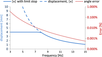
Figure 4. Proof mass displacement amplitude and error resulting from the small angle approximation vs rolling frequency and speed. A rim diameter of 15 inches (38 cm) and a tire rolling diameter of 20 inches (51 cm) were assumed. Limit stop is at a 4 mm displacement.
Download figure:
Standard image High-resolution imageIn addition to the small angle approximation, the preceding analysis assumes the mass is a point mass, meaning that it has no rotational inertia, and that there are no other forces acting on it. Although the point mass assumption introduces only negligible errors, there will always be other forces acting on the proof mass if energy is to be extracted. A more detailed analysis, including the other forces acting on the proof mass, follows in sections 3 and 4.
3. Prototype design and discussion
A few practical application-related constraints must be considered that will largely drive the design implementation presented here. First, the system must generate enough power to support transmissions once per minute, even at very slow speeds (<15 kph). This constraint necessitates relatively large allowable displacements (∼ ±2.5 mm). The primary reason behind this constraint is that it is important for the system to generate enough power to send an initial pressure measurement during the first minute of driving, which is typically quite slow. The constraint could potentially be obviated by the inclusion of long-term energy storage, such as a rechargeable battery. However, a rechargeable battery would add too much cost to the system and would present its own reliability concerns. Second, the height (i.e., size in the radial direction) must be small because of the tire and rim geometry, which rules out a cantilever structure extending in the radial direction or an actual pendulum as shown in figure 2.
We implemented a curved track with a radius smaller than the rim radius to implement the offset pendulum dynamics. This solution is illustrated in figure 5. The proof mass is a steel ball bearing that rolls back and forth along the curved track. This system can withstand the very large static centripetal load without deflection while still maintaining low friction motion in the tangential direction. To improve the harvesting of energy at low rotating frequencies, we employed spring loaded end stops.
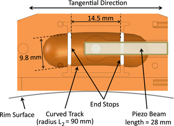
Figure 5. Illustration of energy harvester concept, side view. Ball rolls back and forth in the curved track between the two end stops. As it passes through the center of the track, it deflects the piezoelectric beams.
Download figure:
Standard image High-resolution imageThe transducers are two piezoelectric beams running along the length of the track, one on each side. The beam and proof mass make contact through a smaller ball held in a conical hole along the side of the track. As the proof mass rolls past the smaller ball, the smaller ball gets pushed out and deflects the piezoelectric beam. This process is illustrated in figure 6, which shows the device from the top with the piezoelectric beams running along each side of the device.
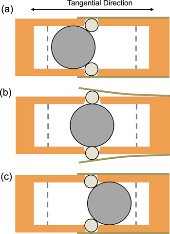
Figure 6. Illustration of piezoelectric beam actuation, top view. When the proof mass ball is in the position on the left (a), the piezoelectric beams are undeflected. When the proof mass ball is in the center position (b), the piezoelectric beams are deflected. When the proof mass ball passes through to the right (c), the beams return to their undeflected position. Thus, there are two piezoelectric deflection cycles per proof mass oscillation period.
Download figure:
Standard image High-resolution imageWe decided to use piezoelectric rather than electromagnetic transduction because, at low frequencies, the voltage from the electromagnetic system would be very low and require more complex power electronics, and therefore have reduced efficiency. As piezoelectric devices are generally stiff, they are best actuated in a high-force, low-displacement mode. The mechanical actuation system shown in figure 6 is essentially a force amplification mechanism, so the lower-force, higher-displacement motion of the proof mass is converted to a higher-force, lower-displacement motion for the piezoelectric beam. A second benefit of the actuation system shown is that it is inherently immune to reliability concerns from over-travel.
4. Modeling and analysis of nonlinear dynamics
The interaction of the proof mass with the piezoelectric beams, as well as with the spring loaded end stops, alters the effective spring constant of the system. Figure 7 shows the effective spring force on the proof mass at very slow speeds (i.e., neglecting the effect of the centripetal acceleration). The location of the spring loaded end stops is clearly indicated. Throughout most of the proof mass motion, there is a negative spring constant, meaning that the spring force pushes the proof mass away from the zero displacement point. The gravitational force on the proof mass is also shown for the case where the tangential axis is aligned with gravity. The figure shows that the gravitational force is strong enough to push the proof mass through its entire range of motion at a low speed. From a design perspective, it is desirable to maximize the amount of force transferred to the piezoelectric element. In the quasistatic case (as shown in figure 7), the force transfer would be maximized if the effective spring force just reaches, but stays below, the gravitational force. The design case shown in figure 7 leaves a small margin for error. All relevant parameter values for the design case shown in figures 7– 9 are shown in table 1.
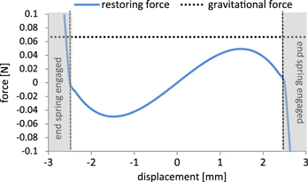
Figure 7. Effective spring (restoring) force and gravitational force on the proof mass over its range of motion. Gravitational force assumes the tangential axis is aligned to gravity.
Download figure:
Standard image High-resolution imageTable 1. Parameter values for design case shown in figures 7– 9. Parameters are defined in equation (6).
| Parameter | Value | Unit | Comment |
|---|---|---|---|
| m | 6.8 | grams | |
| Ac (65 kph) | 628 | m s−2 | |
| Ac (100 kph) | 1470 | m s−2 | |
| kp | 304 | N m−1 | |
| R1 | 4.76 | mm | |
| R2 | 1.59 | mm | |
| Rtr | 80 | mm | |
| L3 | 159 | mm | |
| y | 0 < y < 0.51 | mm | y is maximum at x = 0 |
| α | ±0.92 | deg. | for displacements (x) of ±2.5 mm |
| γ | ±23 | deg. | for displacements (x) of ±2.5 mm |
Figure 7 includes the effect of the end springs (i.e., limit stops) but does not include the equivalent spring effect of the centripetal acceleration. Equation (6) gives the equivalent spring force over all speed ranges, including the effect of centripetal acceleration, but neglects the effect of the spring loaded end stops. The spring force for three different speeds is shown in figure 8. As the speed increases, the effect of the centripetal acceleration becomes more significant. At 65 kph, the system still exhibits negative stiffness, but it is less extreme and through a smaller portion of the range of motion. At 100 kph, the stiffness function is that of a stiffening spring. At higher speeds, the spring will behave more linearly, and therefore more like an offset pendulum system, as described in section 2.

where Ac is the centripetal acceleration, α is the angle between the rim and track at some point along the track (x)—given by α = x(1/Rtr –1/L3), where Rtr is the radius of the track in which the proof mass travels and L3 is the distance from the center of the wheel to the tire pressure sensor location, kp is the stiffness of the piezoelectric beam, y is the deflection of the piezoelectric beam, and γ is the angle between the centers of the proof mass ball and the smaller piezoactuating ball and is given by γ = sin−1(−x/(R1 + R2))—where R1 and R2 are the radii of the proof mass and actuator balls, respectively.
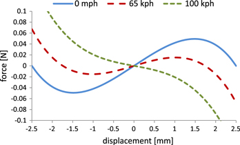
Figure 8. Effective spring (restoring) force at three different speeds showing the changing shape of the spring force as a function of speed. Area in which the spring loaded end stops are active (|x| > 2.5 mm) is not shown.
Download figure:
Standard image High-resolution imageFigure 9 offers another view of the same behavior. The initial negative stiffness results in a double-well potential function characteristic of bistable oscillators. As the speed increases, the height of the unstable equilibrium point lowers until the potential function is characteristic of a stiffening spring. At very high speeds, the spring will approach the behavior of a linear spring.

Figure 9. Shape of the nonlinear potential function. Three speeds shown: near 0 kph (very slow), 65 kph, and 100 kph. At high speeds, the potential function approaches that of a standard linear spring.
Download figure:
Standard image High-resolution imageThe simplified equations of motion are given in (7) and (8)

where b is the coefficient of viscous damping, Cr is the coefficient of rolling friction, a is the effective piezoelectric force factor, V is the voltage across the piezoelectric device, Cp is the capacitance of the piezoelectric device, and I is the current flowing into the electronic load.
The left side of equation (7) shows the inertial term (7/5m
 ), viscous damping term (b
 ), rolling friction term [mAc
Cr
sgn(
), rolling friction term [mAc
Cr
sgn( )], piezoelectric coupling term (aV), and the equivalent restoring force as given in equation (6). Note that the 7/5 coefficient in front of the inertial term is a result of the rotational inertia of the proof mass. If the mass were treated as a point mass, the coefficient would be 1. In practice, the rotational inertia only has a significant effect near the speed at which the friction components overwhelm the motion of the system. This effect will be discussed in more detail in the following section. Note also that the effect of friction between the proof mass and the actuator balls is neglected in equation (7). This friction force varies from zero to a maximum value when the piezoelectric beams are at their maximum extension. For the design case under consideration, the maximum friction force between the proof mass and actuator balls is approximately equivalent to the rolling friction between the proof mass and housing at a speed of 13 kph, beyond which speed the rolling friction quickly dominates. The important dynamics of the system are essentially unaffected by omitting this friction force.
The two parts of the equivalent restoring force can be written as a function of the displacement variable x, as shown in equations (9) and (10). If L3 = 2L2, the condition for resonance in equation (5), the first term of the restoring force reduces to equation (11)


Although perhaps not immediately obvious, the equivalent restoring force is similar to the standard cubic stiffness of a Duffing oscillator. In particular, the right side of equation (10) could be rewritten as k1x + k3x3. As shown in figure 10, if k1 = −0.01 and k3 = 0.0075, the resulting restoring force as a function of x is almost exactly the same as that given by equation (10), with values taken from the prototype in figure 14. Taken together, the entire restoring force could be written as (k0 + k1)x + k3x3, where k0 = mΩ2 and increasingly dominates as rotation speed increases.

Figure 10. Effective spring force for the energy harvester prototype and for a general cubic spring of the form k1x + k3x3, where k1 = −0.01 and k3 = 0.0075.
Download figure:
Standard image High-resolution image5. Simulation results
We created a numerical simulation of the system to explore its behavior and optimize the design. As the system is highly nonlinear, we use the convergence to an average power ( ), given by equation (12), as the appropriate performance metric for this nonlinear system. The electrical load is assumed to be a matched resistor (RL
), calculated as RL
= (1/(ΩCp
))*ζ/(4ζ2 + k4)1/2 where k is the system coupling coefficient and ζ is the viscous damping ratio [3]. This equation is for a resonant piezoelectric system, which admittedly has simpler dynamics than the current system. Nevertheless, we considered it sufficiently accurate to explore the important dynamics. At each frequency, the system simulation is allowed to run for a sufficient number of forcing periods (n) such that any transients die out; then, equation (12) is applied over n periods to get an average power generation value
), given by equation (12), as the appropriate performance metric for this nonlinear system. The electrical load is assumed to be a matched resistor (RL
), calculated as RL
= (1/(ΩCp
))*ζ/(4ζ2 + k4)1/2 where k is the system coupling coefficient and ζ is the viscous damping ratio [3]. This equation is for a resonant piezoelectric system, which admittedly has simpler dynamics than the current system. Nevertheless, we considered it sufficiently accurate to explore the important dynamics. At each frequency, the system simulation is allowed to run for a sufficient number of forcing periods (n) such that any transients die out; then, equation (12) is applied over n periods to get an average power generation value

where n is the number of forcing periods, T = 2π/Ω is the period of the forcing oscillation, V(t) is the generated voltage, and RL is the load resistance.
Given the extra forces from the interaction with the piezoelectric beam and the spring loaded end stops, the system is no longer always resonant, as implied by figure 2 and equation (5). However, the bandwidth of the device is still significantly enhanced compared to a simple linear oscillator. Figure 11 shows the simulated rms voltage across a matched resistor and the power output vs frequency.

Figure 11. Simulated output voltage and power vs rotation frequency. Piezoelectric generator is terminated with a matched resistor.
Download figure:
Standard image High-resolution imageThe simulated output shown in figure 11 indicates that the proof mass motion, and thus voltage and power output, drop dramatically at about 160 kph. The simulation models both viscous and rolling friction. At very high speeds, the displacements naturally go down and the rolling friction goes up due to an increasing normal force between the proof mass and track. At around 160 kph, the friction overwhelms the motion of the system. The simulation shown in figure 11 assumes a coefficient of rolling friction of 0.0005. Although this value has not been directly measured, it is consistent with experimental power output at high speeds measured in both laboratory and road tests.
One disadvantage of this particular design is that it is very sensitive to misalignment about the wheel rotation axis. If the track in which the proof mass rolls is misaligned, a portion of the centripetal acceleration will couple into the direction of motion of the proof mass (the tangential direction). The tangential excitation is ±1 G. If the component of the relatively static centripetal acceleration that couples into the direction of motion is greater than 2 G, the proof mass will be pinned against one limit stop and not move at all. Figure 12 shows the allowable misalignment versus speed for a typical tire/rim combination. To operate at high speeds, the misalignment must be significantly below 1 degree. The prototypes we built and tested had a self-alignment mechanism built in and that operated well up to approximately 155 kph. However, it is worth noting that this particular design requires a self-alignment mechanism to operate robustly. The sensitivity to misalignment can be reduced by reducing the track radius below one-half the wheel radius. In fact, we used both simulated and tested prototypes with smaller track radii in an effort to improve high-speed performance. However, we found that the self-alignment mechanism was sufficient and, although the smaller track radii resulted in better high-speed operation in simulation, that advantage rarely carried over to actual laboratory and road tests.
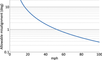
Figure 12. Allowable harvester misalignment vs speed for a typical wheel. If the harvester is misaligned by more than this, the proof mass will not move and there will be no power output.
Download figure:
Standard image High-resolution imageThe data shown in figure 11 was collected by simulating a wheel turning at a constant speed. The simulation was repeated for each wheel rotation speed. Simulating the system as the wheel speeds up and slows down again reveals further dynamic characteristics. Figure 13 shows a simulation of the proof mass displacement as the speed of the car increases from 8 to 225 kph. The gray area in the figure shows the position output over time as the speed slowly ramps up. The black dots are 'stroboscopic' points indicating the output position at each Ω/2π, where Ω is the rolling frequency of the wheel. Regions in which the output is periodic, at the same frequency as the input, appear as dark black lines. Areas in which the black dots appear randomly indicate a chaotic response, which is characteristic of bistable oscillators under certain circumstances. Chaotic behavior is exhibited below 65 kph during both the up-sweep and the down-sweep. This is consistent with the potential function shown in figure 9. From 65 to 190 kph, the oscillation amplitude on the up-sweep is much higher than on the down-sweep. This behavior is consistent with a stiffening spring [22, 23], which the harvester exhibits at moderate to high speeds because of the interaction of the restoring forces imposed by the piezoelectric beam actuation mechanism and the centripetal acceleration. This stiffening behavior is also evident in the 100 kph curve in figure 8. The nonlinear stiffening behavior is not apparent in the single speed simulations shown in figure 11. In practice, this stiffening effect provides a stable operation characteristic over a wide frequency range, as will be shown from the laboratory and road testing.
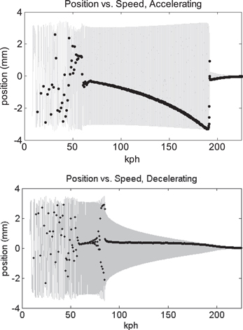
Figure 13. Simulated position of the proof mass vs speed accelerating from 8 to 225 kph (up-sweep) and then decelerating from 225 back to 8 kph (down-sweep). The gray regions show the proof mass position over time, whereas the black dots are 'stroboscopic' points indicating the position of the proof mass each Ω/2π, where Ω is the rolling frequency of the wheel.
Download figure:
Standard image High-resolution imageThe acceleration/deceleration for the data shown in figure 13 was 5.5 kph s−1. Simulations were run with acceleration/deceleration values ranging from 3.5 to 22 kph s−1. The essential characteristics of the output data do not change based on acceleration/deceleration. The onset of chaos and large stable oscillations occur at the same speeds, regardless of acceleration/deceleration values within the range simulated.
The amplitude of oscillation at slow to moderate speeds is primarily determined by the location of the limit stops. Therefore, as long as the system can 'push through' the center region, where the piezoelectric beams are at maximum deflection, the value of system parameters, such as mass, viscous damping, and rolling friction, do not have a large effect on the system's dynamic performance. The primary effect of mass, damping, and friction on dynamic performance are to determine the speed at which the proof mass ceases to undergo large amplitude oscillations. As the mass increases, the speed at which friction overcomes the oscillation also increases and vice versa. As the damping and rolling friction increase, the critical speed decreases.
The speed over which the response is chaotic is primarily determined by the shape of the potential energy function, as shown in figure 9. For speeds at which the potential function is highly bistable, the response appears chaotic. As the speed increases, the potential function transforms from a bistable to a stiffening spring. For the design case under consideration, this occurs at approximately 65 kph. The shape of this potential function is determined by the proof mass, piezoelectric beam stiffness, and geometry of the curved track, proof mass, and actuator balls. These factors will influence the effective restoring force, as shown in equation (6), and therefore, the potential energy function.
6. Laboratory and road test results
Several prototypes based on this concept were built and tested. One example is shown in figure 14. Three experimental setups were used to validate the behavior of the harvesting system. The first was a laboratory setup (see figure 15(a)), in which a wheel is rotated at a controlled speed with the harvester prototype attached. This setup allows more detailed investigation of the harvesting system. The second is the road test setup, shown in figure 15(b), in which the harvester is attached to the rim inside an inflated tire and interfaced with an electrical feedthrough to a data acquisition system that continuously measures output voltage across a load resistor, among other signals such as temperature. In the third test setup, the harvester powers an actual tire pressure monitor device developed by LV Sensors Inc. (see figure 16). The entire self-powered TPMS prototype system is attached to the rim inside an inflated tire using a belt around the rim. The measurement variable of interest in this case is the time between transmissions. Extensive tests were performed with all three test setups.

Figure 14. Prototype device used for road testing. (a) Fully assembled device with piezoelectric beam along outside and actuator ball visible protruding from conical hole. (b) Inside of harvester device showing curved track, proof mass, and spring loaded end stops.
Download figure:
Standard image High-resolution image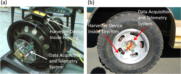
Figure 15. Laboratory (a) and road (b) test setups. The harvester prototype is attached to a rim. The signal from the harvester is acquired using a wireless data acquisition system attached to the wheel hub.
Download figure:
Standard image High-resolution image
Figure 16. Full TPMS prototype system. The storage capacitor, power electronics, programming pins, and TPMS chipset are attached to a printed circuit board on the harvester package.
Download figure:
Standard image High-resolution imageFigure 17 shows the harvester voltage at three different speeds measured on the laboratory test setup. The signal becomes significantly noisier at higher speeds, as expected. The peak voltage is relatively constant across a wide voltage range, as designed. However, at very high speeds, there is a slight drop in peak voltages.

Figure 17. Piezoelectric voltage vs time. Measurements taken on laboratory setup at three different rotation speeds.
Download figure:
Standard image High-resolution imageFigure 18 shows the voltage output across the load resistor measured with the first road test setup. The measured voltage is a little lower in magnitude and the pulse is narrower than the simulated voltage. These facts likely indicate an assembly tolerance issue, such as a small gap between the piezoelectric beam and the actuator ball placed in the conical hole (see figure 6) when the proof mass is at one end or the other. The result is that the piezoelectric beam does not deflect quite as far as designed. The effect of noise was not included in the simulations; however, it is clear in the test data (both laboratory and road test data). As the speed increases, the effect of the noise becomes more pronounced.
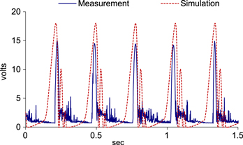
Figure 18. Simulated and measured open circuit voltage output. Tire is rolling at 16 kph.
Download figure:
Standard image High-resolution imageThe circuit architecture for the third test setup is shown in figure 19. The energy requirement for one measurement and transmission cycle depends, to a certain extent, on the state machine programmed into the TPMS. Each car manufacturer has its own specification for data gram length, number of repeats, etc. The state machine we used for the system demonstration tests required 375 μJ per measurement and transmission cycle. Therefore, the system requires 6.25 μW of power generation on average to achieve one transmission per minute. We designed the system to achieve at least 10 μW through a load resistor at very slow speeds (see figure 11) to account for inefficiencies in the power circuitry.
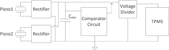
Figure 19. Circuit architecture for full system test setup. Piezoelectric elements charge a storage capacitor. Once the voltage on the storage capacitor is high enough to support a measurement and transmission cycle, the comparator closes the switch connecting the storage capacitor to the ½ voltage divider and the TPMS.
Download figure:
Standard image High-resolution imageThe power circuitry operates as follows. The comparator circuit shown in figure 19 waits for the voltage across the storage capacitor (Cstor ) to reach an upper threshold (Vhigh ). Then it connects the TPMS load to the Cstor through a charge pump voltage divider that reduces the voltage by one-half. Once the voltage on the Cstor drops to a lower threshold (Vlow ), the comparator disconnects the TPMS load while the Cstor recharges. Thus, the measurement variable of interest is the time between transmissions. Note that the TPMS system has an onboard voltage regulator so its power supply does not need to regulated, it only needs to remain inside the operation window of the TPMS. We selected the size of the storage capacitor, the threshold voltages, and the reduction ratio from the charge pump voltage divider to meet the energy requirements for TPMS operation. Furthermore, we selected the threshold voltages to be close to one-half the open circuit voltage generated by the piezoelectric elements (see figures 17 and 18). In this particular case, the threshold voltages are 7.3 and 3.8 volts and Cstor is 40 μF. The amount of energy supplied to the TPMS during one measurement and transmission cycle is therefore Ecyc = ½ Cstor (Vhigh 2–Vlow 2), which is 777 μJ or roughly double what is really needed. Because we have not included the parasitic current draw of the comparator, voltage divider, and leakage currents, we sized the system to provide extra energy per cycle. The TPMS system takes a measurement, sends a data packet, waits for a minor delay, and then continues to transmit the data packet until its power is shut off. Clearly, the system could be further optimized. However, for our purposes, this configuration provided a robust demonstration piece.
We calculated the expected time between transmissions based on a dynamic simulation of the system that provides power transfer to the storage capacitor, or power generation, versus speed. The expected time between transmissions is then simply the energy usage per cycle (Ecyc ) divided by power generation at a given speed. For example, at 10 kph, the expected power generation is 10 μW. Therefore, the expected time between transmissions would be 78 s.
Figure 20 shows the results of road tests conducted with the system just described. Both experimental data from multiple runs and simulation output are shown. The system performs well, meaning that it supports a transmission more than once per minute, from speeds of 10 to 155 kph. The slow speed performance is particularly impressive, as the system can support more than one transmission per minute down to speeds of 10 kph. Note that, particularly at slow speeds, the system generates more power than expected. This is most likely because of extra noise imparted to the system (i.e., road noise, bumps, etc) that is not modeled but contributes to power generation. At high speeds, above 155 kph, the increased rolling friction overcomes the inertial forces and the time between transmissions climbs rapidly. Overall, the system behaves marginally better than the simulations predict.

Figure 20. Experimental data showing the time between TPMS transmissions for a rim-mounted energy harvester. Data shown for multiple tests on three different devices. The red dotted line shows the expected time between transmissions based on the simulation.
Download figure:
Standard image High-resolution image
7. Conclusions
We demonstrated an energy harvesting architecture for a rotating environment in which the axis of rotation is horizontal, or perpendicular to gravity. We have applied this harvester architecture to a TPMS. The architecture uses the dynamics of an offset pendulum to increase the operational bandwidth. The combination of restoring forces acting on the system, including centripetal acceleration and restoring forces from the piezoelectric beams, creates a nonlinear bi-stable oscillator at slow speeds that shifts to a stiffening oscillator at higher speeds. Although not always resonant, the frequency response of the system is significantly broader than a standard linear oscillatory system. The harvester was tested in both a laboratory setting and on the road. The test results show a good match to dynamic models, indicating that they can be used profitably as a design tool. During road tests, the harvester was able to support better than one transmission per minute in the speed range of 10–155 kph, and more than three transmissions per minute from 32–155 kph.
Acknowledgments
The authors gratefully acknowledge the modeling contributions of Jeffrey Tola and assistance with road testing provided by Ron Chisholm.