

Abstract
Most previous studies on nonlinear Lamb waves are conducted using mode pairs that satisfying strict phase velocity matching and non-zero power flux criteria. However, there are some limitations in existence. First, strict phase velocity matching is not existed in the whole frequency bandwidth; Second, excited center frequency is not always exactly equal to the true phase-velocity-matching frequency; Third, mode pairs are isolated and quite limited in number; Fourth, exciting a single desired primary mode is extremely difficult in practice and the received signal is quite difficult to process and interpret. And few attention has been paid to solving these shortcomings. In this paper, nonlinear S0 mode Lamb waves at low-frequency range satisfying approximate phase velocity matching is proposed for the purpose of overcoming these limitations. In analytical studies, the secondary amplitudes with the propagation distance considering the fundamental frequency, the maximum cumulative propagation distance (MCPD) with the fundamental frequency and the maximum linear cumulative propagation distance (MLCPD) using linear regression analysis are investigated. Based on analytical results, approximate phase velocity matching is quantitatively characterized as the relative phase velocity deviation less than a threshold value of 1%. Numerical studies are also conducted using tone burst as the excitation signal. The influences of center frequency and frequency bandwidth on the secondary amplitudes and MCPD are investigated. S1–S2 mode with the fundamental frequency at 1.8 MHz, the primary S0 mode at the center frequencies of 100 and 200 kHz are used respectively to calculate the ratios of nonlinear parameter of Al 6061-T6 to Al 7075-T651. The close agreement of the computed ratios to the actual value verifies the effectiveness of nonlinear S0 mode Lamb waves satisfying approximate phase velocity matching for characterizing the material nonlinearity. Moreover, the ratios derived from the primary and secondary horizontal displacements generated from nonlinear S0 mode Lamb waves are closest to the real value, which indicates that using horizontal displacements is more suitable for detecting evenly distributed microstructural changes in large thin plate-like structure. Successful application to evaluating material at different levels of evenly distributed fatigue damage is also numerically conducted.
Export citation and abstract BibTeX RIS
1. Introduction
Early evaluation and continuous tracking of material microstructural changes, the evolution of damage and degradation is demanding in many structural components. A variety of nondestructive methods have been developed for efficient damage detection and evaluation. Ultrasonic method is the most powerful one and has been exploited for many years [1, 2]. Conventional ultrasonic inspection method is based on linear theory, and normally depends on measuring particular parameters, i.e., sound velocity, attenuation, or transmission and reflection coefficients of the propagating waves to determine the elastic properties of a material or to detect defects. However, the traditional ultrasonic testing method is just sensitive to gross damages, but much less sensitive to the changes in the microstructure or evenly distributed degradation.
An alternative way to overcome the shortcoming of the liner theory based ultrasonic method is nonlinear ultrasonics. When a monochromatic sinusoidal ultrasonic wave with a finite amplitude interrogates a crystalline solid, the interaction of the acoustic wave with microstructural features would lead to distortion of the initial ultrasonic waveform and thus higher harmonic waves are generated. Initial investigation by Breazeale and Thompson [3] put forward elastic material nonlinearity as predominant cause for higher-order harmonics generation. The changes in the microstructure features, i.e., dislocation [4–8], persistent slip bands [9], and precipitation characteristics [10, 11] contribute to higher harmonics were also analytically investigated. Evaluation of fatigue damage using nonlinear ultrasonics receives considerable interest. Cantrell and Yost [12] theoretically and experimentally studied fatigued microstructures, and a lot of researchers have applied nonlinear ultrasonics to assessing fatigue damage in various materials such as structural steel [13], nickel-base superalloy [14] and Ti-6Al-4 V [15]. And nonlinear ultrasonics was also used to predict fatigue life [16]. Besides of fatigue damage, it was also employed to evaluate other failure mechanisms, i.e., hardening [17], thermal aging [18] and radiation damage [19]. In these theoretical or experimental studies, bulk waves are used.
Compared to point-to-point inspection style of ultrasonic bulk waves, Lamb waves technology [20–23] provides a high-efficient and cost-effective inspection method as Lamb waves are able to travel a very long distance with little loss in energy and it can be also successfully used to interrogate physically inaccessible areas of structures and components. Nonlinear Lamb waves have emerged as an attractive alternative for detecting microstructural changes preceding the initiation of macro-scale damages as they combine the early damage detection capabilities of nonlinear ultrasound with the efficient large-scale inspection approach of Lamb waves. However, the multi-mode characteristic and dispersive nature of Lamb waves make the nonlinear Lamb waves propagation much more complicated than that of nonlinear bulk waves. Compared to the study of nonlinear acoustics starting in the 18th century [24], nonlinear Lamb waves have made considerable progress during the past two decades. Chillara and Lissenden [25] reviewed nonlinear ultrasonic guided wave nondestructive evaluation quite recently.
A lot of researchers have theoretically studied the cumulative second harmonic generation in plates. These scholars include Deng [26, 27], De Lima and Hamilton [28], Chillara and Lissenden [29], Müller [30], Matsuda and Biwa [31], Matlack [32], Liu [33] and so on, and their considerable contributions put forward the development of nonlinear guided waves. These analytical investigations derived two necessary conditions for cumulative second harmonic generation, i.e., phase velocity matching and non-zero power flux, and proposed some mode pairs satisfying these two conditions. Along with these theoretical studies, experimental studies were conducted using S1–S2 mode pair (S1 is the primary Lamb wave mode and the S2 is the second harmonic) to characterize material nonlinearity [34, 35], tensile plasticity-driven damage [36], fatigue damage [37], thermal fatigue [38] and creep damage [39–41]. Besides of S1–S2 mode pair, A2–S4 mode pair [42] was also employed to experimentally investigate fatigue damage. Also, S1–S2 and S2–S4 mode pairs are used by Rauter and Lammering [43] to numerically study contact acoustic nonlinearity caused by micro-structural as well as global material and geometrical nonlinearities. Recently, Liu et al [44, 45] has extended the nonlinear Lamb waves to hollow circular cylinders.
The above investigations on cumulative second harmonic generation are based on phase velocity matching and non-zero power flux conditions. However, there exist some limitations. First, in real applications, as the excitation signal is normally a tone burst with a finite bandwidth, strict phase velocity matching only exist at the center frequency of the whole bandwidth; Second, excited center frequency of the primary mode is not exactly equal to the true phase-velocity-matching frequency; Third, mode pairs are isolated and quite limited in number; Fourth, exciting a single desired primary mode of the mode pairs is extremely difficult in practice and some unwanted modes would be generated simultaneously making the received signal quite difficult to process and interpret; Lastly, time-frequency analysis is needed to process the received complicated signals in which some unwanted Lamb modes overlap with the desired primary and secondary modes. And short-time Fourier transform (STFT) method is frequently used in the previous studies [34–37, 46]. However, when using STFT, selecting an optimum window size is quite difficult and an improper window size would lead to the wrong results [36].
Few attention has been paid to solving the above shortcomings. In this study, nonlinear S0 mode Lamb waves at low-frequency range satisfying approximate phase velocity matching and non-zero power flux conditions is proposed to overcome these limitations and to detect large-scale distributed microstructural changes in thin structures. The merits of using nonlinear S0 mode Lamb waves at low-frequency range are stated as follows. First, phase velocity approximate matching conforms to real applications in which a tone burst with a finite bandwidth is used as the excitation signal; Second, nonlinear S0 mode Lamb waves at low-frequency range is more robust, as it is phase velocity approximate matched; Third, the centered fundamental frequency can lie at an interval of low-frequency range not just some isolated points on the phase velocity dispersion curve; Fourth, exciting a single desired S0 mode Lamb wave is much easier and few unwanted modes would be generated, as the primary centered frequency is reduced to low-frequency range; Lastly, an ordinary Fourier Transform method is adequate to process the obtained waveform.
Phase velocity mismatching has been investigated by Matsuda and Biwa [47]. However, in Matsuda and Biwa's work, S1–S2 mode pair was used and the limitations were still not resolved. Nonlinear S0 mode Lamb wave technique has been used for detecting micro cracks [48–50]. However, in these studies, it was used for quantifying local contact acoustic nonlinearity, not for characterizing evenly distributed material nonlinearity and cumulative second harmonic generation was thus not considered. Recently, Chillara and Lissenden published two papers [51, 52] related to nonlinear S0 mode Lamb waves. In [51], the authors numerically studied harmonic generation from the primary S0 and A0 modes for the purpose of demonstrating that interaction of Lamb wave modes of the same nature generate symmetric modes and the group velocity matching is unnecessary. And the authors did not investigate cumulative second harmonic generation from the primary S0 Lamb waves. In [52], the authors' attention was mainly focused on studying localized microstructural changes, and nonlinear S0 mode Lamb waves only at 0.5 MHz was used and phase velocity approximate matching was not discussed. In a word, in these above researches, nonlinear S0 mode Lamb waves were employed not for the purpose of solving the limitations of nonlinear Lamb waves based on phase velocity matching. Although the idea of phase velocity mismatching and use of nonlinear S0 mode Lamb waves are not new, it is the first time that we combine the idea of phase velocity approximate matching and nonlinear S0 mode Lamb wave together to overcome the shortcomings of nonlinear Lamb waves using mode pairs, to explore the conditions of cumulative second harmonic generation and to detect evenly distributed microstructural changes.
In this article, several major concerns are mainly discussed. First, the displacement amplitude of second harmonic with the propagation distance considering the phase velocity deviation is studied. Second, in order to use the cumulative effect of the second harmonic generated from S0 mode Lamb waves for the detection of microstructural changes, the maximum cumulative propagation distance (MCPD within which the displacement amplitude of second harmonic increases with the propagation distance) with the phase velocity deviation is investigated, and furthermore, the maximum linear cumulative propagation distance (MLPCD within which the amplitude of second harmonic grows linearly with the propagation distance) is also studied by using linear regression analysis. Third, approximate phase velocity matching is quantitatively defined. The rest of this paper is organized as follows. Analytical study is given in section 2. Numerical study is elaborated in section 3. Effectiveness is verified in section 4. Application to evaluating fatigue damage at different levels is studied in section 5. Conclusions are draw at last in section 6.
2. Analytical study
2.1. Cumulative second harmonic generation of Lamb waves under phase velocity matching and non-zero power flux conditions
The nonlinear wave equation associated with displacement vector for a homogenous solid plate is given by [26, 27, 40]
where  denotes the mass density,
  and
and  are the second-order elastic (SOE) constants of the solid, and
  is the displacement vector which is assumed to be expressed as

where  and
and  represent the displacement vectors of the fundamental frequency and the second-harmonic waves. Substituting equation (2) into (1), two equations are derived [26]

where  is calculated from
  using
using  instead of
  .
.
For a solid plate, suppose a Cartesian coordinate system is illustrated in figure 1 [26]. The coordinate origin is located in its central plane, the  axis is along the direction of wave propagation and the
  axis is along the plate thickness. The plate thickness is
  Given a line source parallel to the
  axis and located at
  by analyzing the nonlinear interaction of partial bulk waves and the restriction of the two boundaries of the solid plate, Deng [26] derived the analytical solution of the cumulative second-harmonic displacement field written as
where  or
or  in the subscript indicates that the corresponding quantity is related to the longitudinal or transverse wave, respectively;
  in the subscript is 1 or 2;
  or
or  denotes the angle between the
  axis and
  or
or  which is the wave vector of partial longitudinal or transverse wave as shown in figure 1;
 and
and  are the unit vectors of
 and
and  axis;
axis;  and
and  are the locations of wave propagation;


 and
and  (
( are expressed in the following equation [26]


where 
 and
and  are the third-order constants;
  is the amplitude of partial longitudinal wave;
 and
and  are given by
 and
and  in which
 and
and  refer to the angular frequency of primary Lamb wave, the phase velocity of primary Lamb wave and the velocity of transverse wave (
 or longitudinal wave (
 and
and  are expressed by
 ![${m}_{31}=[(\kappa +4\mu /3){\alpha }_{L}^{2}+\kappa -2\mu /3]\mathrm{sin}\;{\theta }_{L}$](https://content.cld.iop.org/journals/0964-1726/25/4/045023/revision1/smsaa1912ieqn55.gif) and
and  .
.

Figure 1. Partial bulk wave fields of Lamb-mode propagation. ' ' represents the displacement vector.
Download figure:
Standard image High-resolution image2.2. Second harmonic generation of S0 mode Lamb waves at low frequencies under approximate phase velocity matching and non-zero power flux conditions
Previous study [51] has already demonstrated that the second harmonic mode is also S0 when the primary Lamb wave mode is S0. According to the theory reported by Deng [26, 53], the analytical solution to second harmonic generation of S0 mode Lamb waves is expressed in equation (11)

where  denotes the second harmonic displacement field of S0 mode Lamb waves,
  is expressed in equation (5) and
  is given by
  in which
  and
and  refer to phase velocities of the fundamental and the second harmonic Lamb wave. The second harmonic displacement components along the
  and
and  axes are given as
According to equations (12) and (13),  increases with
  in the form of sine function within the first quadrant, and when
 reaches to its first maximum value. Therefore,
  is obtained. Solving this equation, a MCPD
  is derived and it is expressed as

2.3. Analytical results
Consider an aluminum Al-6061-T6 plate with the thickness of 2 mm. The material properties are shown in the first row of table 1. The phase velocity dispersion curves for the plate are shown in figure 2(a).
Table 1. Material properties of Al-6061-T6 [54] and Al-7075-T651 [55].
| Material | ρ (kg m−3) | κ (GPa) | μ (GPa) | A (GPa) | B (GPa) | C (GPa) |
|---|---|---|---|---|---|---|
| Al-6061-T6 | 2704 | 67.6 | 25.9 | −416 | −131 | −150.5 |
| Al-7075-T651 | 2810 | 70.3 | 26.96 | −351.2 | −149.4 | −102.8 |

Figure 2. Dispersion curves for an Al-6061-T6 plate with the thickness of 2 mm: (a) phase velocity; and (b) group velocity.
Download figure:
Standard image High-resolution image2.3.1. Amplitudes of the second harmonic with propagation distance
Using equations (12) and (13), and assuming that the excitation source is located at  the horizontal and vertical amplitudes of the second harmonic generated from the primary S0 mode Lamb waves are derived. Figures 3(a)–(f) illustrate examples of horizontal and normal amplitudes of the second harmonic with the propagation distance. In figure 3, the horizontal and vertical scales are
  and
and 
 and
and  are the fundamental and second harmonic frequencies; and
  refers to the relative deviation of the phase velocities between the primary wave and second harmonic, and it is expressed as
  Several observations are noted. First, horizontal and vertical amplitudes of the second harmonic increase with propagation distance in the form of sine function within the first quadrant, and they reach their peaks at the same propagation distance. Second, the horizontal amplitudes are much larger than vertical amplitudes at low fundamental frequencies of 50, 100, 150 and 200 kHz, however, smaller at high frequencies of 400 and 500 kHz. This observation is in accordance with results reported in the previous study [27]. Third, the first peak appears at longer propagation distances at low fundamental frequencies than at high fundamental frequencies.

Figure 3. Examples of amplitude of second harmonic with propagation distance: (a) 
 and
and  (b)
(b) 
 and
and  (c)
(c) 
 and
and  (d)
(d) 
 and
and  (e)
(e) 
 and
and  and (f)
 and
and  = 10.72%.
Download figure:
Standard image High-resolution image2.3.2. Maximum amplitudes of the second harmonic with the fundamental frequency
Figure 4 illustrates the logarithmic scaling of the maximum horizontal and vertical amplitudes of the second harmonic with the fundamental frequency from 50 to 500 kHz with an increase of 50 kHz. It is obviously shown that both the horizontal and vertical amplitudes of the second harmonic are decreased with the increase of fundamental frequency. And the maximum horizontal amplitude decreases much more dramatically than maximum vertical amplitude. Consequently, at larger fundamental frequencies, the maximum horizontal amplitude is smaller than maximum vertical amplitude.

Figure 4. The logarithmic scaling of the maximum amplitudes of second harmonic with the fundamental frequency.
Download figure:
Standard image High-resolution image2.3.3. The MCPD with the fundamental frequency
Using equation (14), the MCPD  at different fundamental frequency is easily calculated. The sixth column in table 2 shows the MCPD with the fundamental frequency from 25 to 700 kHz with an increment of 25 kHz. The maximum fundamental frequency of 700 kHz is selected to make sure that the frequency of the second harmonic is under the cut-off frequency of S1 mode. It is obviously illustrated that the MCPD
  is decreased dramatically, as the fundamental frequency is increased.
Table 2.
The MCPD  and MLCPD
  at different fundamental frequencies.
 
|
 
|
 
|
 
|
 
|
 
|
 
|
|---|---|---|---|---|---|---|
| 25 | 50 | 5351.18 | 5350.62 | 0.01 | 511 424.55 | 378 054 |
| 50 | 100 | 5350.62 | 5348.37 | 0.04 | 63 531.34 | 46 900 |
| 75 | 150 | 5349.68 | 5344.57 | 0.10 | 18 650.48 | 13 801 |
| 100 | 200 | 5348.37 | 5339.17 | 0.17 | 7764.72 | 5734 |
| 125 | 250 | 5346.66 | 5332.07 | 0.27 | 3908.06 | 2886 |
| 150 | 300 | 5344.57 | 5323.15 | 0.40 | 2213.99 | 1636 |
| 175 | 350 | 5342.08 | 5312.25 | 0.56 | 1359.04 | 1004 |
| 200 | 400 | 5339.17 | 5299.14 | 0.75 | 883.40 | 652 |
| 225 | 450 | 5335.84 | 5283.55 | 0.98 | 599.09 | 443 |
| 250 | 500 | 5332.07 | 5265.15 | 1.26 | 419.49 | 309 |
| 275 | 550 | 5327.85 | 5243.47 | 1.58 | 300.99 | 223 |
| 300 | 600 | 5323.15 | 5217.95 | 1.98 | 220.02 | 162 |
| 325 | 650 | 5317.96 | 5187.83 | 2.45 | 163.08 | 121 |
| 350 | 700 | 5312.25 | 5152.12 | 3.01 | 122.09 | 90 |
| 375 | 750 | 5305.98 | 5109.49 | 3.70 | 91.98 | 68 |
| 400 | 800 | 5299.14 | 5058.15 | 4.55 | 69.51 | 51 |
| 425 | 850 | 5291.67 | 4995.63 | 5.59 | 52.53 | 39 |
| 450 | 900 | 5283.55 | 4918.55 | 6.91 | 39.55 | 29 |
| 475 | 950 | 5274.73 | 4822.27 | 8.58 | 29.59 | 22 |
| 500 | 1000 | 5265.15 | 4700.79 | 10.72 | 21.93 | 16 |
| 525 | 1050 | 5254.75 | 4547.73 | 13.45 | 16.10 | 12 |
| 550 | 1100 | 5243.47 | 4360.33 | 16.84 | 11.77 | 8.7 |
| 575 | 1150 | 5231.24 | 4148.58 | 20.70 | 8.72 | 6.4 |
| 600 | 1200 | 5217.95 | 3937.35 | 24.54 | 6.68 | 4.9 |
| 625 | 1250 | 5203.52 | 3751.45 | 27.91 | 5.38 | 4.0 |
| 650 | 1300 | 5187.83 | 3599.99 | 30.61 | 4.52 | 3.3 |
| 675 | 1350 | 5170.75 | 3480.09 | 32.70 | 3.94 | 2.9 |
| 700 | 1400 | 5152.12 | 3385.34 | 34.29 | 3.53 | 2.6 |
2.3.4. The MLCPD with the fundamental frequency
It should be noted that within MCPD  the amplitude of second harmonic does not grow linearly. In order to efficiently apply the nonlinear S0 mode Lamb wave to evaluating microstructural changes, the MLCPD
  within which the amplitude of second harmonic increases linearly is also investigated by using linear regression analysis. As the amplitudes of second harmonic with the propagation distance show the similar trend for both horizontal and vertical displacements, only the horizontal amplitude data is used for calculating MLCPD
  .
.
For a specific fundamental frequency, suppose the variable  (
( is the propagation distance and
  (
( the corresponding horizontal amplitude of the second harmonic, and
  denotes the propagation distance equal to MCPD
  and
and  the maximum amplitude of the second harmonic. And (
 (
(
 ... (
... (
 form the points from the first one to the point at the MCPD
  An example at the fundamental frequency of 100 kHz is shown in figure 5.

Figure 5. An example showing (
 (
( ).
).
Download figure:
Standard image High-resolution image2.3.4.1. The MLCPD realization by linear regression analysis
The diagram to derive the MLCPD  is elaborated in the following steps and illustrated in figure 6. In the linear regression analysis, a threshold value for the parameter adjusted
  is set to 0.99.
- Step 1: Prepare the dataset (
 ().
(). - Step 2: Find the maximum i and set its value to M.
- Step 3: Draw the scatter plot for dataset ( ().
- Step 4: Conduct the linear regression and compute the adjusted.
- Step 5: Compare the computed value of the adjusted with 0.99. If the value of the adjusted is larger than 0.99, set the value of the current M to M' and the MLCPD If not, delete the point ( from ( ( and go back to step 2.


Figure 6. The flow chart to derive the MLCPD.
Download figure:
Standard image High-resolution image2.3.4.2. The MLCPD results
Using the method proposed in section 2.3.4.1, the MLCPD  at different fundamental frequency is derived. The seventh column in table 2 shows the MLCPD
  with the fundamental frequency from 25 to 700 kHz with an increase of 25 kHz. Similar to the trend of MCPD
  the MLCPD
  decreases significantly with the fundamental frequency. By comparing the sixth and seventh columns of table 2, it is observed that the MLCPD is about 74% of its corresponding MCPD at each fundamental frequency. It should be noted that the MLCPD at each fundamental frequency is close related to the adjusted
  .
.
2.3.5. Nonlinear S0 mode Lamb wave satisfying phase velocity approximate matching
Cumulative effect, especially linear cumulative effect, of the second harmonic is useful and helpful in real applications. However, the efficiency of cumulative effect reduces rapidly with the phase velocity deviation, as the amplitudes of second harmonic decrease with the fundamental frequency and the MCPD and MLCPD are decreased dramatically with the phase velocity deviation. In order to efficiently detect microstructural changes in large thin structures, it is better to use nonlinear S0 mode Lamb wave with the relative phase velocity deviation less than a threshold value of 1%. In this paper, the phase velocity approximate matching is regarded as the relative phase velocity deviation less than 1%.
3. Numerical study
Analytical study in section 2 is based on the monochromatic continuous primary Lamb wave. However, Lamb wave tone bursts with finite duration are commonly used in practical applications. In this section, tone burst with a finite duration is used as the excitation signal. The influence of center frequency on the amplitudes of the second harmonic and MCPD is studied at the center frequencies of 100 and 200 kHz with a certain tone-burst cycle. And the effect of frequency bandwidth on the second harmonic and MCPD is also investigated with the tone-burst cycles of 10, 20 and 40 at the center frequency of 100 kHz. COMSOL software is used for numerical simulations.
3.1. Finite element simulation setup
3.1.1. Schematic of the finite element simulation model
The schematic of 2D plane strain model with loads and boundary conditions is illustrated in figure 7. The thickness of the plate is chosen to be 2 mm. The material is aluminum 6061-T6 and its properties are shown in the first row of table 1. Uniform loads are enforced on the left end of the plate to excite the intended primary S0 mode Lamb waves. Fixed boundary condition is applied to the right end and the upper and lower surface of the plate are free.

Figure 7. Schematic of the 2D finite element simulation model.
Download figure:
Standard image High-resolution image3.1.2. Excitation signal
A tone burst consisting of  cycles with a specified center frequency
  is used as the excitation signal and it is formulated in equation (15)

where  refers to the amplitude of the excited signal, and it is set to be 10 MPa.
An example of the excitation temporal waveforms and their frequency spectrums with different cycles are illustrated in figures 8(a) and (b), respectively. It is shown that the more cycles of temporary waveform, the narrower of its frequency bandwidth.

Figure 8. Excitation signal with  20 and 40 and
  (a) temporal waveform and (b) frequency spectrum.
Download figure:
Standard image High-resolution image3.1.3. Element size and time step
In general, a higher-order element type, a denser mesh and smaller time step will give a more accurate simulation result, but will also cost more in terms of calculation time and computer resources. In order to obtain adequate accuracy and high efficiency, a second-order rectangular element type is used, and the maximum element size and time step is adopted according to the [56]


where  is the element size and
  the time step;
  and
and  are shortest wavelength and highest frequency of interest, respectively.
In this paper, we consider the second harmonic generation,  refers to the largest upper limit of the frequency bandwidth of the second harmonic. The parameters used in finite element simulations are listed in table 3, where
  and
and  are the center frequency of the primary and secondary wave, respectively.
Table 3. Parameters used in finite element simulations.
 
|
 
|
 
|
 
|
 
|
|---|---|---|---|---|
| 100 | 200 | 250 | 1 | 1 × 10⁻⁷ |
| 200 | 400 | 500 | 0.5 | 5 × 10⁻⁸ |
3.2. Numerical results
3.2.1. Representative temporal waveform and its spectrum
Figure 9 shows the representative signal obtained from the primary S0 mode Lamb waves with ten cycles at the center frequency of 200 kHz propagating at 400 mm. Its temporary waveform and spectrum are illustrated in figures 9(a) and (b) respectively. From the spectrum, second harmonics are clearly observed.

Figure 9. Vertical displacement received from the primary S0 mode Lamb waves at the center frequency of 200 kHz propagating at 400 mm: (a) temporary waveform and (b) spectrum.
Download figure:
Standard image High-resolution image3.2.2. The influence of center frequency
In this section, numerical simulations are conducted using ten-cycle excitation signal at the center frequencies of 100 and 200 kHz.
3.2.2.1. Amplitudes of the second harmonic with the propagation distance
Figure 10 illustrate horizontal and normal amplitudes of the second harmonic with the propagation distance. It is clearly observed that the horizontal and vertical amplitudes of second harmonic grow with the propagation distance in the form of sine function within the first quadrant which is in accordance with the analytical study. The horizontal and vertical amplitudes show the similar trend and they reach their maximum amplitudes at the same propagation distance. Similar to analytical results, horizontal amplitudes are larger than vertical amplitudes at the center frequencies of 100 and 200 kHz.

Figure 10. Amplitude of second harmonic with propagation distance: (a) 
 and (b)
 = 0.75%.
Download figure:
Standard image High-resolution image3.2.2.2. The effect of center frequency on the maximum amplitudes of the second harmonic
The maximum amplitude of the second harmonic at the center frequency of 100 kHz is larger than at 200 kHz. The detailed values are shown in table 4, where  and
and  refer to the horizontal and vertical maximum amplitudes of the second harmonic, respectively. In table 4, the horizontal and vertical amplitudes of the second harmonic decrease with the center frequency. And the maximum horizontal amplitude decreases much more dramatically than maximum vertical amplitude. These findings are similar with the analytical results.
Table 4. The maximum amplitudes of the second harmonic at the center frequencies of 100 and 200 kHz.
 
|
 
|
 
|
 
|
 
|
 
|
 
|
|---|---|---|---|---|---|---|
| 100 | 200 | 5348.37 | 5339.17 | 0.17 | 3.985 × 10⁻⁶ | 4.778 × 10⁻⁷ |
| 200 | 400 | 5339.17 | 5299.14 | 0.75 | 9.185 × 10⁻⁷ | 2.385 × 10⁻⁷ |
3.2.2.3. The effect of center frequency on MCPD and MLCPD
In figure 10, the first maximum amplitude appears at larger propagation distance at the center frequency of 100 kHz than at 200 kHz. The sixth column of table 5 shows the MCPD at the center frequencies of 100 and 200 kHz. It is illustrated that MCPD reduces significantly with the center frequency. And numerical results of MCPD at the center frequency of 100 and 200 kHz are shorter than the analytical results at the corresponding fundamental frequencies. One possible reason for this phenomenon is that the primary Lamb wave for the analytical study is monochromatic and continuous while for the numerical study is tone burst with finite duration.
Table 5.
The MCPD  and MLCPD
  at the center frequencies of 100 and 200 kHz.
 
|
 
|
 
|
 
|
 
|
 
|
 
|
|---|---|---|---|---|---|---|
| 100 | 200 | 5348.37 | 5339.17 | 0.17 | 4750 | 3500 |
| 200 | 400 | 5339.17 | 5299.14 | 0.75 | 550 | 400 |
Numerical results of MLCPD are obtained using the linear regression method described in section 2.3.4, and shown in the seventh column of table 5. It is illustrated that the MLCPD is also about 74% of its corresponding MCPD at the center frequencies of 100 and 200 kHz, which is identical to the analytical study. Nonlinear S0 mode Lamb waves with lower frequency is more suitable for evaluating large-scale structures with microstructural changes.
3.2.3. The influence of frequency bandwidth
In this section, numerical simulations are conducted using the excitation signal of 10, 20 and 40 cycles at the center frequencies of 100 kHz.
3.2.3.1. The influence of frequency bandwidth on amplitudes of the second harmonic
Figures 11(a) and (b) show horizontal and vertical displacement amplitudes of the second harmonic with the propagation distance considering different cycles. It is illustrated that the horizontal and vertical amplitudes of second harmonic increase linearly with the cycles of the primary Lamb wave. In real applications, it is feasible to use a large cycle to obtain a large amplitude of the second harmonic.

Figure 11. Amplitude of second harmonic with propagation distance considering different cycles: (a) horizontal displacement and (b) vertical displacement.
Download figure:
Standard image High-resolution image3.2.3.2. The influence of frequency bandwidth on MCPD
Figures 12(a)–(f) show horizontal and vertical displacement amplitudes of the second harmonic with the propagation distance between 4500 and 5000 mm with the excitation signal of 10, 20 and 40 cycles, respectively. It is clearly observed that the MCPDs are the same with a value of 4750 mm for the primary Lamb wave of 10, 20 and 40 cycles. MCPD is constant with the change of frequency bandwidth.

Figure 12. Amplitudes of second harmonic with propagation distance between 4500 and 5000 mm considering different cycles: (a)–(c) horizontal displacement and (d)–(f) vertical displacement.
Download figure:
Standard image High-resolution image4. Verification of effectiveness
In this section, S1–S2 mode pair with the fundamental frequency at 1.8 MHz, the primary S0 mode Lamb waves at the center frequencies of 100 and 200 kHz are used to detect the material nonlinearities of aluminum plate with the thickness of 2 mm.
4.1. Nonlinearities modeling
For an undamaged isotropic homogeneous solid plate with purely elastic behavior, two types of nonlinearities, i.e., the material nonlinearity and geometric nonlinearity, need to be taken into account. The material nonlinearity comes from the nonlinear elastic properties of the material, while the geometric nonlinearity from the transformation of wave motion equation from the Eulerian to the Lagrangian coordinates.
The stress–strain relation in a nonlinear elastic solid can be expressed, with a second-order approximation, as follows [57]

where  denotes the stress tensor;
  and
and  are the strain tensors;
  is the SOE tensor expressed with
  and
and  and
and  is a tensor accounting for both the material and geometric nonlinearities simultaneously, which can be expressed as [58]

where
In equations (19) and (20),  and such in its form with different index orders are the Kronecker delta;
  and such in its form denote the fourth-order identity tensors;
 is the third-order elastic (TOE) tensor describing the material nonlinearity, and the last three terms in equation (19) altogether address the geometric nonlinearity. As illustrated in equation (20),
  is determined by three third-order constants A, B and C, which can be treated as the inherent properties of the material, to be measured experimentally.
In a one dimensional analysis as for longitudinal waves, equation (18) is simplified as [46, 59]

where 
 and
and  denote the stress, strain, and Young's Modulus of the material, respectively.
  is the second order Young's Modulus that introduces the nonlinear effects [60] to the material. Solving equations (18)–(20) yields

Taking the ratio of the two Young's Moduli, the nonlinear parameter  for an isotropic material can be defined as [46, 59]

In equation (23), it can be obviously seen that  is dominated by four material property parameters (Young's Modulus and three third order elastic constants). Hence, for a specific material without any damage or plastic deformation,
  can be regarded as an inherent material property quantifying the material nonlinearity of the medium.
Using Lamb wave, the nonlinear parameter  can be determined by [35]

where  is the wave number and
  the propagation distance;
  and
and  are the the displacement amplitudes at the fundamental and second harmonic frequencies of the received signal, respectively;
  is the frequency dependent function, which has no explicit expression.
Since  is unavailable, a relative nonlinear parameter
  is constructed to quantify the degree of nonlinearity as [35]

According to the theory [34, 35] stated that the relative nonlinear parameter  is linearly proportion to the nonlinear parameter
  and the propagation distance if the measured Lamb wave modes are cumulative, the relative nonlinear parameter
  could be also expressed as [34, 35]

The relative nonlinear parameter  contains essential information reflecting the nonlinear properties of wave propagation.
4.2. Finite element simulations setup
Two aluminum plates with the thickness of 2 mm, i.e., Al 6061-T6 and Al 7075-T651 are used. Their material properties listed in table 1. The schematic of the finite element simulation model is shown in figure 7. Numerical simulation parameters are shown in table 6.
Table 6. Parameters used in finite element simulations of material nonlinearity detection.
| No. | Phase matching | Primary mode | Secondary mode |
 
|
 
|
 
|
 
|
|---|---|---|---|---|---|---|---|
| 1 | Strict | S1 | S2 | 1800 | 3600 | 0.05 | 5 × 10⁻⁹ |
| 2 | Approximate | S0 | S0 | 100 | 200 | 1 | 1 × 10⁻⁷ |
| 3 | Approximate | S0 | S0 | 200 | 400 | 0.5 | 5 × 10⁻⁸ |
4.3. S1–S2 mode pair
4.3.1. Typical waveform
Figure 13 shows the temporal presentation of a typical signal captured by recording the horizontal displacement at 100 mm from the left end of the aluminum Al-6061-T6 plate. In order to extract the required signal features to construct the relative nonlinear parameter  time-frequency analysis is necessary. In this section, STFT and the Morlet wavelet transform [61] are used respectively to process the received signal. In STFT analysis, the window size is carefully selected such that sufficient details of both time and frequency information of the waveform could be retained. Compared with STFT, the Morlet wavelet transform is robust as user's optimization of the parameters is unnecessary. From the spectrogram obtained from STFT or the Morlet wavelet transform, it is readily feasible to extract the amplitude profiles at fundamental and double frequencies as a respective function of time. Figures 14(a) and (b) show an example of amplitude profiles extracted from the spectrogram obtained by STFT. From figure 2(b), it is clearly that the fundamental mode S1 and its second harmonic mode S2 are the first arrivals at their corresponding frequencies. Therefore, in figures 14(a) and (b), the first peak value of the amplitude profiles at the fundamental frequency and second harmonic frequency are identified as
  (of S1 mode) and
  (of S2 mode), respectively.

Figure 13. A typical time-domain signal captured by recording the horizontal displacement at 100 mm from the left end of the aluminum Al-6061-T6 plate.
Download figure:
Standard image High-resolution image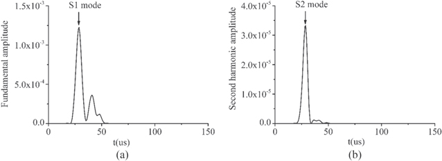
Figure 14. Amplitude profiles extracted from the spectrogram obtained by STFT: (a) at the fundamental frequency of 1800 kHz (of S1 mode); and (b) at the second harmonic frequency of 3600 kHz (of S2 mode).
Download figure:
Standard image High-resolution image4.3.2. The relative nonlinear parameter β' with propagation distance
4.3.2.1. The relative nonlinear parameter β' obtained from STFT
Figures 15(a) and (b) show the relative nonlinear parameter  with propagation distance
  and best fit functions in
  where k is the slope proportion to the nonlinear parameter
  and b is a constant. The relative nonlinear parameters
  in figures 15(a) and (b) are calculated from horizontal and vertical displacements, respectively. It is obviously illustrated that a linear increase in the relative nonlinear parameter
  with increasing propagation distance for both aluminum plates, which corresponds to a cumulative second harmonic generation in both specimens for the selected S1–S2 mode pair. The best fit slope k, which is proportion to the nonlinear parameter
  for Al 6061-T6 is higher than that for Al 7075-T651. The ratio of the nonlinear parameter of Al 6061-T6 to that of Al 7075-T651 calculated from the horizontal displacement is
  =
=  and from the vertical displacement is
  =
=  = 15.95/12.37 = 1.29.

Figure 15. The relative nonlinear parameter β' obtained from STFT: (a) the horizontal displacement; and (b) the vertical displacement with propagation distance using nonlinear Lamb S1–S2 mode pair.
Download figure:
Standard image High-resolution image4.3.2.2. The relative nonlinear parameter β' obtained from the Morlet wavelet transform
In figure 16, it is clearly shown that the relative nonlinear parameter  is increased linearly with the propagation distance, which presents a linear cumulative second harmonic generation in both specimens for S1–S2 mode pair. The ratio of the nonlinear parameter of Al 6061-T6 to that of Al 7075-T651 computed from the horizontal displacement is
  =
=  and from the vertical displacement is
  =
=  = 29.47/25.11 = 1.17.

Figure 16. The relative nonlinear parameter β' obtained from the Morlet wavelet transform: (a) the horizontal displacement; and (b) the vertical displacement with propagation distance using nonlinear Lamb S1–S2 mode pair.
Download figure:
Standard image High-resolution image4.4. The primary S0 mode at the center frequency of 100 kHz
The temporal presentation of a typical signal is shown in figure 9. To extract the required signal features to construct the relative nonlinear parameter  the Fourier transform is adequate.
In figure 17, it is clearly shown that the relative nonlinear parameter  grows linearly with the propagation distance for both aluminum plates, which indicates a cumulative second harmonic generation in both specimens for the primary S0 Lamb wave mode at the center frequency of 100 kHz, as the propagation distance of 500 mm is much shorter than the MLCPD of 3550 mm. The S0 mode Lamb wave is linearly cumulative within this propagation distance. The ratio of the nonlinear parameter of Al 6061-T6 to that of Al 7075-T651 calculated from the horizontal displacement is
  =
=  and from the vertical displacement is
  =
=  = 4.853/4.169 = 1.16.
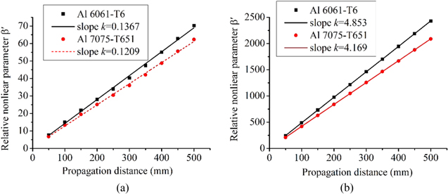
Figure 17. The relative nonlinear parameter β' calculated from: (a) the horizontal displacement; and (b) the vertical displacement with propagation distance using the primary S0 mode Lamb wave at the center frequency of 100 kHz.
Download figure:
Standard image High-resolution image4.5. The primary S0 mode at the center frequency of 200 kHz
In figure 18, it is obviously illustrated that the relative nonlinear parameter  is increased linearly with the propagation distance, which presents a linear cumulative second harmonic generation in both specimens for the selected primary S0 Lamb wave mode at the center frequency of 200 kHz, as the propagation distance of 300 mm is shorter than the MLCPD of 400 mm. The ratio of the nonlinear parameter of Al 6061-T6 to that of Al 7075-T651 computed from the horizontal displacement is
  =
=  and from the vertical displacement is
  =
=  = 17.66/14.96 = 1.18.

Figure 18. The relative nonlinear parameter β' calculated from: (a) the horizontal displacement; and (b) the vertical displacement with propagation distance using the primary S0 mode Lamb wave at the center frequency of 200 kHz.
Download figure:
Standard image High-resolution image4.6. Results comparisons and discussions
Using equation (23), the actual ratio of the nonlinear parameter of Al 6061-T6 to that of Al 7075-T651 is  The values of the ratio of the nonlinear parameter of Al 6061-T6 to that of Al 7075-T651 are summarized in table 7, where 'H' and 'V' represent that results are calculated from the horizontal and vertical displacement.
Table 7. Comparison of the ratio of the nonlinear parameter of Al 6061-T6 to that of Al 7075-T651.
| S1–S2 mode | S0 mode at 100 kHz | S0 mode at 200 kHz | |||||||
|---|---|---|---|---|---|---|---|---|---|
| The ratio | Actual value | STFT | the Morlet wavelet | FFT | |||||
| H | V | H | V | H | V | H | V | ||

|
1.12 | 1.25 | 1.29 | 1.16 | 1.17 | 1.13 | 1.16 | 1.15 | 1.18 |
In table 7, there are several observations. First, the ratios of nonlinear parameter of Al 6061-T6 to Al 7075-T651 calculated from S1–S2 mode processed by the Morlet wavelet transform, the primary S0 mode at the center frequencies of 100 and 200 kHz are close to the actual value, which verifies the effectiveness of nonlinear S0 mode Lamb waves satisfying approximate phase velocity matching for characterizing the material nonlinearity.
Second, the ratios of nonlinear parameter computed from S1–S2 mode processed by the STFT have a relatively high deviation from the actual value. The possible reason is that the imperfect parameters, i.e., window size and overlapping rate are selected in STFT when deriving the primary and secondary amplitudes. However, the ratios of nonlinear parameter obtained from the processing method of the Morlet wavelet transform are much closer to the actual value. Therefore, the Morlet wavelet transform is proposed to process the received signals obtained from nonlinear Lamb waves using mode pairs which are phase velocity strictly matched.
Third, the ratios computed from the primary S0 mode at the center frequency of 100 kHz are closer to the actual value than derived from 200 kHz. This observation suggests using nonlinear S0 mode Lamb waves with smaller phase velocity deviation to get more accurate results.
Fourth, the ratios from the horizontal displacements of S0 at 100 and 200 kHz are the first and second closest values to the real value. This may result from the reason that the horizontal displacement filed of S0 mode at the low-frequency range across the thickness the plate is almost constant, while the vertical displacement field of S0 mode and the displacement of S1 and S2 are dominated near the surface of the structure. Examples of wave structure are illustrated in figures 19(a)–(d), and they are plotted by the Modeshape software developed by LAMSS [63]. In this sense, horizontal displacements of nonlinear S0 mode at low-frequency range satisfying approximate phase velocity matching is more suitable for efficiently evaluating evenly distributed microstructural changes. And S1–S2 mode pair satisfying phase velocity matching is proper for detecting microstructural damages near the surface of the structure [52].

Figure 19. Wave structure: (a) S0 mode at 100 kHz; (b) S0 mode at 200 kHz; (c) S1 mode at 1.8 MHz and (d) S2 mode at 3.6 MHz.
Download figure:
Standard image High-resolution image5. Applications to evaluating evenly distributed fatigue damage at different levels
In this section, nonlinear S0 mode Lamb waves at the centered fundamental frequency of 100 kHz is used to evaluate the evenly distributed fatigue damage at different levels.
The TOE material properties of Al 7075-T651 at different levels of fatigue damage are shown in table 8 [55]. The schematic of the finite element simulation model is shown in figure 7. Numerical simulation parameters are shown in second row of table 6.
Table 8. Third-order elastic material properties of Al-7075-T651 at different levels of fatigue damage [55].
| Fatigue life |
 
|
 
|
 
|
|---|---|---|---|
| 0% | −351.2 | −149.4 | −102.8 |
| 40% | −358.3 | −153.7 | −113.2 |
| 80% | −359.8 | −155.9 | −115.3 |
Figure 20 illustrates the relative nonlinear parameter β' calculated from horizontal displacement with the propagation distance considering different levels of fatigue damage. It is shown that at each level of fatigue damage, the relative nonlinear parameter β' increases linearly with the propagation distance. As the slope of the fitting line is proportion to the nonlinear parameter β, the nonlinear parameter β is increased with the percentage of fatigue life.

Figure 20. The relative nonlinear parameter β' calculated from horizontal displacement with the propagation distance considering different levels of fatigue damage.
Download figure:
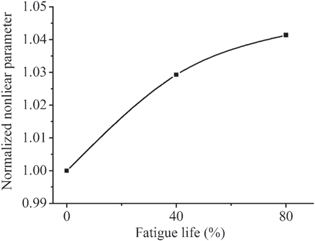
Standard image High-resolution imageFigure 21 shows that the increase in normalized nonlinear parameter is dramatically during the initial stages of fatigue life, and then progresses more slowly towards high percent of fatigue life. This behavior is in agreement with previous results for fatigue damage measured with nonlinear longitudinal [12, 14], Rayleigh [62], and S1–S2 Lamb waves [37].
Figure 21. The normalized nonlinear parameter with the percent of fatigue life.
Download figure:
Standard image High-resolution image
6. Conclusions
In this paper, nonlinear S0 mode Lamb wave at low-frequency range satisfying approximate phase velocity matching is proposed to overcome the limitations of nonlinear Lamb waves satisfying strict phase velocity matching and non-zero power flux conditions. Analytical study is firstly conducted by assuming that the excitation signal is monochromatic and continuous. Analytical results show that horizontal and vertical displacement amplitudes of the second harmonic increase with the propagation distance in the form of sine function within the first quadrant and reach their peaks at the same propagation distance. The maximum amplitudes of second harmonic reduces with the fundamental frequency. The MCPD decreases dramatically with the fundamental frequency. As the secondary amplitude doesn't grow linearly within the MCPD, a method based on linear regression analysis with a threshold value of 0.99 for the parameter adjusted  is proposed to derive the MLCPD. And the MLCPD is about 74% of its corresponding MCPD at each fundamental frequency. Based on analytical study, in order to efficiently detect microstructural changes in large thin plate, nonlinear S0 mode Lamb wave satisfying approximate phase velocity matching is quantitatively defined as the relative phase velocity deviation less than a threshold value of 1%. Then, numerical study is investigated using tone burst with a finite duration as the excitation signal. The influences of center frequency and frequency bandwidth on the secondary amplitudes and MCPD are studied. The secondary amplitudes with the propagation distance and the maximum secondary amplitudes with the centered fundamental frequency show the similar trends with the analytical study. Numerical results also illustrate the MCPD is decreased dramatically with the centered fundamental frequency. However, MCPDs obtained from numerical study are shorter than those derived from analytical investigation. The secondary amplitudes increase almost linearly with the cycles of the primary Lamb wave. But the MCPD is constant with the increase of cycles. Next, the close agreement of the ratios of nonlinear parameter of Al 6061-T6 to Al 7075-T651 calculated from S1–S2 mode processed by the Morlet wavelet transform, the primary S0 mode at the center frequencies of 100 and 200 kHz to the actual value verifies the effectiveness of nonlinear S0 mode Lamb waves satisfying approximate phase velocity matching for characterizing the material nonlinearity. Also, it is shown that using the primary and secondary horizontal displacements generated from nonlinear S0 mode at low-frequency range satisfying approximate phase velocity matching is more suitable for efficiently evaluating evenly distributed microstructural changes. At last, nonlinear S0 mode Lamb waves at the centered fundamental frequency of 100 kHz is successfully applied to characterize different levels of fatigue damage. It should be noted that the MLCPD should be firstly calculated at a certain center frequency before using nonlinear S0 mode Lamb waves. Experimental study will be conducted in the following research.
Acknowledgments
The work described in this paper was supported by grant from the Research Grants Council of the Hong Kong Special Administrative Region, China (Project No. CityU 122513) and National Natural Science Foundation of China (Project No. 51575422).