
Abstract
In this paper, a new calibration method for mechano-luminescence (ML) thin film sensors was proposed to enable quantitative full-field strain measurements in pixel-level resolution for the first time along with two standard reference test methods. The proposed method has a distinct advantage of its facet-free full-field strain sensing capability with pixel-level resolution. For the ML sensor, standard reference test methods were proposed for developing calibrated relationships between ML light intensity and effective strains: (1) uniaxial tensile reference test and (2) non-uniform strain reference test. From the reference tests, two different calibration models were developed in a recurrence equation form and validated measuring general strain distributions on different experimental specimens. Verified finite element (FE) simulation results were compared with ML effective strains to confirm its accuracy. The comparisons of the ML effective strains with FE simulation results showed that the calibration models can acceptably measure full-field strains. Limitations, sources of errors, suggestions for improving accuracy and practical considerations were also discussed. A conclusion of this research is that the proposed method enables ML sensing films to measure quantitative full-field strain distributions.
Export citation and abstract BibTeX RIS

Original content from this work may be used under the terms of the Creative Commons Attribution 3.0 licence. Any further distribution of this work must maintain attribution to the author(s) and the title of the work, journal citation and DOI.
1. Introduction
Full-field strain measurements are critically important to quality control of various structural and mechanical components, engineering design, non-destructive testing and research of materials in automotive, aerospace and civil infrastructure industries. There are several traditional methods for measuring strains such as digital image correlation (DIC) [1], photoelastic coatings [2] and Moire interferometric methods [3]. Among these, DIC techniques have been most widely used for its capability of measuring three-dimensional displacement fields. DIC technologies are matured. However, accuracy of measurements is known to be very sensitive to various factors such as facet sizes and steps. As a new stress sensor and non-destructive test method, interests in mechano-luminescence (ML) sensing materials have been growing ever since Xu et al pioneered fundamental understandings of ML mechanisms and their applications to stress sensors [4]. ML sensing technologies have been advanced in various applications such as stress sensors [4, 5], impact sensor [6], damage sensor [7], visualizations of stress distributions in solids [8, 9], stress field near the tip of crack [10], dynamic torsional response [11], quasi-dynamic crack-propagation in solids [12], internal defects of pipes [13], etc. Use of the ML sensing materials for visualization of cracks has also been investigated in the field of structural health monitoring (SHM) [14, 15].
The ML light intensity is proportional to maximum mechanical loading, loading rate and concentration of ML sensing materials. As the photoexcitation power increases, the ML peak light intensity also increases until a certain level of saturation [16]. However there is an upper saturation limit which can be reached by sufficiently long photoexcitation. Due to the complexity with the intensity-based sensing, Someya et al proposed an idea of using two time constants (i.e. rise and decay) for their immunity to the excitation power and concentration of the sensing materials, and their proportionality and inverse proportionality to load amplitude and loading rate, respectively [16, 17]. Kim et al [11] suggested a ML paint-based non-contact torque transducer and demonstrated possibility of measuring dynamic torque in a rotating shaft through a preliminary experimental work. An empirical prediction model for ML light intensity was suggested considering proportionality of the ML light intensity to the applied torque and the rate of applied torque. An important characteristic of ML sensing materials is the dependency on persistent luminescence (PL) decay of the light intensity under stationary loadings [18, 19]. Rahimi et al revealed effects of the stress-free PL decay on the ML phenomena and characterized effects of the stationary stresses and strain rates on the stress-state PL decay of SrAl2O4:Eu2+,Dy3+(SAOED) materials [19]. Recently, Rahimi et al proposed a predictive stress-optics transduction model which can predict ML light intensity from SAOED thin-film coating sensor subjected to in-plane stresses [20]. Effects of the stress, loading rate, stress-free and stress-state PL were investigated in the study. They concluded that relative total light intensity is linearly proportional to the mechanical strain energy. According to the results from the studies, stress-free and stress-state PL decay response of the ML sensing materials is considered one of the limitations to intensity-based measurements of stationary loadings and strains. Therefore, Kim, et al used a technique that continuously photoexcite ZnS:Cu ML particles by 365 nm ultraviolet (UV) light during the measurements [21]. To overcome the PL decaying response of ML materials (i.e. SAOED) and differences by loading conditions, a method of constantly photoexciting ML particles by UV LED lamp above a certain threshold level during the entire loading process was recently suggested [22]. However, existing studies intended to sense component level response such as loading and torque values, etc. There have been no studies on 'quantitative' full-field strain measurements from ML light intensity.
In this paper, a new calibration method for quantitative full-field strain measurements is proposed along with two different standardized reference methods that develop dynamic calibration models. The proposed method are based on the previous studies on ML mechanisms [19, 20]. However, strain measurement by the proposed method is limited to monotonic loading cases. Measurement of strains under dynamic loading is out of the scope in this paper. To make thin-film ML sensor, the ML sensing ceramic powder is mixed with optical epoxy. A comprehensive experimental test data were generated to develop calibration models and used to quantify strain distributions by ML sensing films. The proposed method is validated by measuring the full-field strain values of three different specimens under different loadings including tension, pure shear and bending moment. In the following sections, manufacturing of the ML sensing film and test setup will be described. Reference test methods to generate data used for developing the calibration model will be described in section 3. In section 4, new calibration models for quantitative full-field stress measurements are proposed and followed by experimental verification and validation in section 5 and conclusions in section 6.
2. Experimental tests
2.1. Manufacturing of ML strain sensing film
In order to manufacture ML sensing films, commercial SAOED particles (LumiNova G-300, United Mineral & Chemical Corporation) were mixed with an optical epoxy resin (West System 105/206). Several factors determine characteristics of transient changes of the ML emission from a thin ML sensing film. These factors can be classified into two categories; (1) manufacturing factors (i.e. materials concentration ratio, ML film thickness, epoxy matrix, etc and (2) experimental factors (i.e. effects of the PL, stress rate, and photoexcitation) [19]. In this paper, the manufacturing factors were fixed by selecting a constant mass concentration ratio of epoxy to ML powder (1:1) and by choosing 0.03 inch (0.762 mm) thickness for the ML film. The ML film was fabricated by the doctor blade method and then the cut ML sensing film was coated on the test specimens by using a commercial adhesive (M-Bond 200 from micro-measurements). The doctor blade method is an efficient way to manufacture thin films with a constant thickness [23]. The thickness can be precisely adjusted by the scale of the doctor blade. By using a flat glass plate, the gap between the blade and the glass plate remains constant.
2.2. Experimental procedures
Before carrying out each of the tests, the ML sensing film was consistently photo-excited by a 60 W broadband light source having wavelength range of 400–1000 nm for 2 min to assure it is fully saturated with the same photoexcitation power. Following full saturations of the films, they were aged for a fixed time in the stress-free state to minimize the effect of stress-free PL decay on the ML emission and to obtain higher ML sensitivity. Therefore, ML sensing films attached on the specimens were aged in the dark place for exactly 7 min before the onset of the loading. A charge-couple device (CCD) camera (AVT MANTA G-0.33B) with a consistent setting of gain factor and a fixed exposure time (100 ms) was positioned around 25 cm in the direction normal to the surface of ML sensing films to photograph the ML emission during the loading process. The images were captured at 10 fps (frames per second) and the ML light intensity was read from the captured images. An Instron Material Tester machine with a capacity of 200 kips is synchronized to the image acquisition by the CCD camera so that onset point of loading is matched with the first image. Figure 1 illustrates the schematic experimental test setup and configuration. While capturing the images, ambient light was completely blocked to minimize undesirable influences of the environmental lights on experimental results. The test in the daylight could be difficult due to weak ML light intensity and effects of transient environmental light. However, a dark chamber can be used to make light condition same to the lab environment.
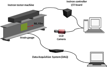
Figure 1. Schematic experimental test setup and configuration.
Download figure:
Standard image High-resolution image3. Reference test methods for developing calibration models
In order to convert ML light intensity to actual strain values, a reference calibration model is needed that covers a wide range of strains and strain rates. In this paper, two different reference test methods are proposed as a standardized method for the proposed ML-based full-field strain sensor. The first one uses both effective strains and ML light intensity directly measured from uniaxial dog-bone tests and the second one uses non-uniform effective strains from a verified finite element analysis (FEA) and ML light intensity measured from a test of a specimen showing non-uniform strain distribution.
In the proposed standardized reference test methods, it is important to consistently age the photo-excited ML sensing film for a fixed time (i.e. 7 min in this paper) both in reference tests and actual tests. By keeping the stress-free PL decay time interval, partial transduction of the mechanical energy into optical energy of photons to compensate PL decay can be minimized and a majority of the mechanical energy can be pumped into the optical energy by ML photon emissions [19].
3.1. Reference test by uniaxial tensile specimens
The first reference test method needs multiple uniaxial tensile tests of standard dog-bone specimens with ML sensing film coated at various strain rates and loadings. One restraint is that the ML sensing films must be prepared through consistent manufacturing process and bonded securely on the specimen throughout the tests. In this case, the ML intensities are averaged over the pixels within the gauge section since the specimen is under constant stress state. The corresponding constant uniaxial strain can be computed from the axial displacement and Poisson ratio of the substrate material. The average light intensity corresponding to the stress on the ML film is calculated by dividing the area integration of ML light intensity in gray level by the area of the region of the interest in pixels. These data are synchronized with the load step data to obtain ML light intensity-force (i.e. stress) curves. The maximum load is limited in a way that the aluminum specimen remains within linear elastic range during the tests since it is intended to measure strains within elastic range of the substrate material. An advantage of the first method is that it can directly measure both strains and corresponding ML intensity, which are deemed as true values. However, it requires more times and labors due to needs for multiple tests.
3.2. Reference test by specimens with non-uniform strains
The second reference test method is to conduct test with a specimen that show a non-uniform strain distribution. An advantage of the second method is that it can generate strain distributions showing a wide range of strains and strain rates even with a single test. Thus, it can save times and labors compared to the first method. Nevertheless, it would not be easy to measure full-field strain distributions within the zone of interests by conventional sensors like strain gauges. Therefore, the best option is to use strains predicted by three-dimensional FEA that is verified by experimental tests. Non-uniform strain states can be easily generated by design of specimens with complex geometries. In this paper, I-beam for four-point bending test was selected to produce non-uniform strain states since stresses on the web between loading point and supports are highly non-uniform. Generally, non-uniform strain states around loading points or notches are generated due to stress concentrations. However, it is worth noting that any irregular shapes of specimens can be used to produce non-uniform strain states.
4. Calibration models for strain measurements
4.1. Selection of strain measures for ML strain sensor
The ML light intensity is a scalar value whereas strains are a tensor. Thus, on a basis of a hypothesis that the ML emission process is most effectively triggered by movement of dislocations within SAOED crystals, the effective strain is determined to be measured from ML light intensity. In metallic materials, dislocations result in yielding and plastic deformation. Obviously, it was evidenced that deviatoric stresses in the ML film are more effective for stimulating the ML process of trap-releasing and recombination with emission centers than hydrostatic or mean stress [24]. The effective strain is analogous to the von Mises stress, which is compared to uniaxial yield stress in the yield criteria of metal plasticity. The von Mises stress corresponds to a certain multiaxial stress state. Analogously, a certain state under multiaxial strains yields an effective strain to be matched with a ML light intensity. The effective strain is a scalar value defined as follows [25]

where  is the effective strain,
 , and
, and  are the normal strain components, and
 and
and  are the engineering shear strain components. For the first reference test under a uniaxial tensile stress state, the effective stress becomes

where  is Poisson ratio (0.33) of the aluminum material (Aluminum Alloy 6061). The ML light intensity is mapped to this effective strain by a calibration model to be proposed in the following subsections. Although it is challenging to achieve perfect isotropy within ML sensing film, it is assumed that ML sensing film shows isotropic material properties.
For the second reference test method, a three-dimensional FE model is used to extract effective strains since stresses can be highly inhomogeneous. Therefore, equation (1) is used for computing effective strains from FEA results.
4.2. A model from uniaxial tensile reference test
In order to create the ML calibration model which predicts the full-field strain values, a series of comprehensive experimental tension tests were conducted on a standard aluminum dog-bone specimen. The test database was prepared under various conditions by varying the loading rates (0.1, 0.2, 0.3, and 0.4 mm s−1) after the stress free PL decay time of 7 min Loads were linearly applied up to 15 kN and each test was repeated three times to minimize the experimental error. After carrying out image processing in MATLAB, an average value of ML light intensity was calculated for each frame over the gauge section on the film. Having a fixed frame rate at 10 fps (frame per second), ML light intensity versus time can be drawn for each time step (0.1 s).
The incremental values of step time  change of the ML light intensity
  a state variable
  and the effective strain from previous step
  are incorporated into the multi-gene genetic programming (MGGP) toolbox [26, 27] to develop a calibration equation of the change of effective strain
  in each time step. The genetic programming (GP) is a widely known evolutionary algorithm that can produce encoded symbolic mathematical expressions from a large training data base. Its backbone algorithm is similar to genetic algorithm that searches for the best individual through cross-over and mutation events. MGGP is a variant of GP which produces a symbolic expression as a weighted linear combination of the outputs from a number of GP individual trees [27]. For each model, the linear coefficients are derived from the training data base using ordinary least square methods. It is known that MGGP's symbolic regression is more accurate and efficient than the GP [27]. More details can be referred to [27].
The general form of the calibration model can be shown as follows

in which  is the change of the effective strain at step
 is the time increment at step
 is the change of the ML light intensity at step
 and
and  is the effective strain at step (n − 1).
  is used in the calibration model to improve the accuracy of the model [28]. For each loading case, the incorporated input data were prepared corresponding to five different step time increments, ∆t = 0.1, 0.2, 0.3, 0.4 and 0.5 s.
A final calibration model equation for the change of the effective strain at step  was obtained as follows
where  indicates an absolute value;
  indicates the natural log;

 and
and  are the model constants and calibrated as

 and
and  for present cases. No physical meanings are assigned to the model constants. The effective strain in each time step can be obtained by accumulation of the changes of the effective strain value of the previous time steps. This proposed model can measure only monotonically increasing effective strains. Although the proposed approach can be attempted to cyclic or dynamic loadings, the topic is out of the scope for this paper.
4.3. A model from non-uniform strain reference test
In this section, a calibration model from the second reference test approach was proposed. It was obtained from a four-point loading test of I-beam. In the test, a ML sensing film was attached on the one-side web of the beam between a loading point and a support as shown in figure 2. Since in this area, in-plane shear stress is dominant and the range of strains and strain rates are vastly wide, the ML light intensities from this area were used for developing a calibration model. The loading was applied linearly up to 150 kN.
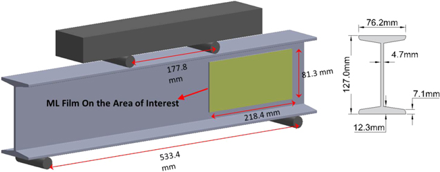
Figure 2. Reference test with four-point loading test of I-beam with ML sensing film attached.
Download figure:
Standard image High-resolution imageA calibration model was developed based on the ML light intensities at 600 arbitrary pixel points on the film and corresponding FE effective strains. The ML light intensities were captured from CCD camera during the loading test and the effective strains were calculated from FEA. Figure 3 shows a view of the three-dimensional FE model of the I-beam used to extract the effective strains.
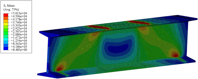
Figure 3. A three-dimensional FE model of the I-beam used to extract effective strains.
Download figure:
Standard image High-resolution imageTo verify the FE model, a strain gauge (Vishay Micro-Measurements SR-4 model WK-06-062AP-350) was installed on the bottom flange of the mid span. The material properties of the FE model were adjusted to elastic modulus 69 000 MPa and Poisson ratio 0.33 until the longitudinal strain by FE simulation matched to the experimental strain value from the strain gauge at the same location. Table 1 summarizes the strains obtained at the highest load (150 kN). In addition, ML light intensities from selected pixel points are regressed to reduce noises from experimental measurements.
Table 1. Longitudinal strain from strain gauge versus that from FE for 150kN load.
| FE simulation | Strain gauge | |
|---|---|---|
| Longitudinal strain at the bottom of the lower flange | 0.002 376 | 0.002 379 |
Table 2. Strain from FE and strain gauge on the top and bottom flanges of the mid spanfor 180kN load.
| FE simulation | Strain gauge | |
|---|---|---|
| Longitudinal strain at the top of the top flange | 0.002 417 | 0.002 365 |
| Longitudinal strain at the bottom of the bottom flange | 0.002 837 | 0.002 869 |
Unlike the calibration model from the uniaxial tensile test, using this test provides different strain rates in one test due to inhomogeneous strain distribution over the area. The strain rates used in the development were between 0.0003 and 0.0021 s−1 and the in-plane shear strains used in the development were between 0.000 08 and 0.0037 s−1.
The incremental values of step time  change of the ML light intensity
  the state variable
  and the effective strain from previous step
  were also incorporated into the MGGP toolbox [26] to develop a calibration equation for the change of effective strain
  in each time step. The variables are the same as those of the model from the uniaxial tensile reference test. Also the data were prepared with five different time increments,
  0.3, 0.4 and 0.5 s.
The final calibration model equation for the change of the effective strain at step  was obtained as follows
where 


 and
and  are the model constants and calibrated as


 for the current case.
5. Measurements of full-field strains using ml sensing film
5.1. Full-field strains by the model from uniaxial tensile reference test
Figure 4 shows plots of comparisons for the true experimental effective strains and measured effective strain versus relative ML light intensity for different loading rates. The results are presented in five different time step increments for each test. These figures demonstrate that the calibration model can accurately relate the measured ML light intensities to the effective strains at various strain rates and time increments. These results also show that the model accuracy is not very sensitive to different step time increments; however, relatively larger errors were observed at time step 0.1 s than other time step increments. The reason for more errors at time step 0.1 s can be found from the nature of the proposed equation in a recurrence form and the prepared data. The original raw ML light intensities were obtained at 10 fps (i.e.  that includes large noises whereas data at other time step sizes were prepared after removing the noises. Another reason is an effect of error accumulations from previous time steps. More number of time steps make more errors accumulated from effective strains predicted at previous steps. These errors also seem to be decreasing as the loading rate increases. According to results from figure 4, the minimum and maximum strains from the reference tests were 0.0001 and 0.0032, respectively. Also the minimum and maximum strain rates were 0.0007 and 0.0025 s−1, respectively.
Figure 4. Experimental and calibrated effective strain versus relative ML light intensity for Δt = 0.1, 0.2, 0.3, 0.4 and 0.5 s under four different loading rates.
Download figure:
Standard image High-resolution imageIn order to validate the calibration model from the uniaxial tensile reference test, thin ML sensing films were applied on a dog-bone specimen with an open-hole specimen. The full-field effective strain values from the proposed calibration model were compared with FE simulation results. The ML films used in the test were so manufactured that the thickness and concentration ratio are as close to the ML film used in the reference tests as possible. The camera setting and conditions for photoexcitation and PL decay time were also kept so that they are as close to those of reference tests as possible.
5.1.1. Uniaxial tensile test of aluminum dog-bone specimen with an open-hole
A uniaxial tensile test was conducted using a dog-bone aluminum specimen with an open-hole. The tensile load was applied linearly up to 45 kN with the loading rate = 0.4 mm s−1. According to FE simulation, areas around the hole in the aluminum specimen are yielded due to stress concentration when the load exceeds 6 kN. Since the calibration model was developed for the specimens within linear elastic range, it is reasonable to compare effective strains from ML and FEA for the loads less than 6 kN. The time increments and the change of the ML light intensity for each step time were recorded through image processing. Effective strains were measured at each pixel by equation (4). The effective strain for each pixel in each step time was obtained by accumulation of the changes of the effective strain values of the previous step times. Figure 5 demonstrates the distribution of the full-field effective strain values at three different loading levels (1.78, 3.57 and 5.35 kN) measured by the calibration model. Also, the effective strain values calculated from the FE simulation (ABQUS 6.13-2) results are presented in figure 5. According to the figure, the present calibration model measured the effective strain with a reasonable accuracy and the results are validated with acceptable accuracy. Maximum strain in figures 5 and 6 is 0.0027, which is within the strain range (0.0001–0.0032) from reference tests. However, the max strain rate was 0.003 s−1, which is slightly over the max strain rate (0.0025 s−1) from reference tests.
Figure 5. Comparison of the ML effective strain (bottom images) and FE effective strain values (upper images) at different loading levels.
Download figure:
Standard image High-resolution image
Figure 6. Effective strain results of the ML calibration model and FE simulation in the vicinity of the open-hole with error percentage distribution at different loading levels.
Download figure:
Standard image High-resolution imageAs it can be seen in figure 5, the distribution of the effective strain from ML sensor is not perfectly symmetric and the area in the right hand side shows higher strain values. The imperfection in specimen set-up in-between the tester machine's grips yielded non-symmetric distribution of the effective strain values on the specimen. The realistic distribution of effective strain values is a considerable advantage of the ML sensor over the FEA since the uncertainty in boundary conditions, material properties, and manufacturing imperfection are the main concerns in standard FE simulations.
The effective strains in the vicinity of the open-hole by the ML sensor and FE simulation are presented with error percentage distribution at different loading levels in figure 6. The error percentages of the calibration model were obtained by simply subtracting the pixel-by-pixel ML effective strains from FE effective strains and dividing the differences by FE effective strains. According to the error percentage figures, the error of the ML sensor decreases by increasing the loading levels. However, it is worth noting that FE results are assumed to be true reference values.
5.2. Full-field strains by the model from non-uniform strain reference test
To verify the calibration model from the non-uniform strain reference test (i.e. the model in section 4.2), the ML effective strains were compared to the effective strains from FEA as shown in figure 7. As described in section 4.2, the calibration model was determined by using test and simulation data from the side span. The results in figure 7 verify that the calibration model has a capability of reproducing the effective strains from the measured ML light intensity. According to results in figure 7, the minimum and maximum strains were 0.0001 and 0.0033, respectively. Also, the minimum and maximum strain rates were 0.000 34 s−1 and 0.0021 s−1, respectively.
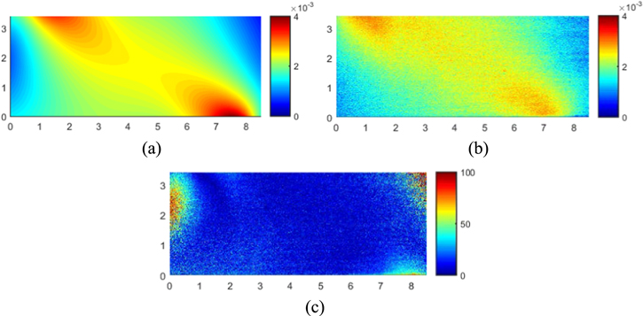
Figure 7. Comparison between (a) effective strain from finite element model, (b) effective strain from ML sensor and (c) the error of the calibration model for the load 150 kN from four-point loading test.
Download figure:
Standard image High-resolution imageResults in figure 7(c) show small errors in the majority of the film area. However, larger errors are particularly shown in two specific areas where the effective strains are too high or too low. The reason for errors in the low strain areas is because the ML sensing film has an inherent material limitation, which is not sensitive enough to react to low strain rates and low strains. The ML light intensity data were selectively collected. Most of data points are from areas with moderate strain level and less data points with high strain level. This makes the calibration model biased to the moderate strain level and causes higher error percentage in the area with high level of strains.
To validate the model's capability of measuring effective strains, thin ML film were applied on two aluminum specimens (1) mid span of the I-beam under four-point load and (2) a standard specimen for pure shear test [29]. The full-field effective strain values from the proposed calibration model were also compared with FE simulation results (ABAQUS 6.13-2) for both tests.
5.2.1. Four-point bending test of the aluminum I-beam
The purpose of this test is to validate measurements of full-field effective strains under typical bending stress states by the proposed calibration model. One side of the web along the center span of an I-beam was coated with a thin ML sensing film with four inches width and three inches height as shown in figure 8. Strain gauges (WK-06-062AP-350) were also installed on the top of the upper flange and on the bottom of the lower flanges for verifying a FE model to be used for comparisons. Table 2 indicates strains on the top and the bottom flanges of the I beam from the FE analysis are acceptably close to ones from the real test. A four-point bending test was conducted by applying the load up to 180 kN so that the I-beam remained in linear elastic range with the maximum loading. Figure 8 displays the experimental test set-up
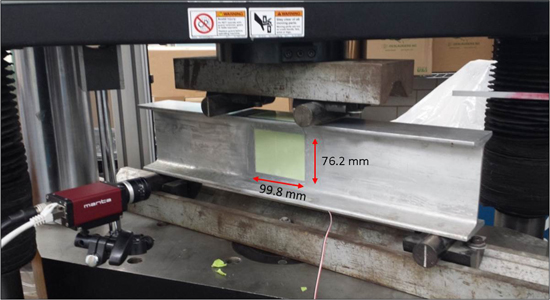
Figure 8. Test setup of the four-point bending test on aluminum I-beam specimen coated with ML sensor.
Download figure:
Standard image High-resolution imageThe distributed effective strain from the FE simulation and ML sensor using the calibration model are presented in figure 9. The error percentages of the results are also shown in figure 9 at different loading levels. According to the results, it can be seen that the errors are reduced as the loading levels increase. It can also be concluded that the calibration model for ML sensor can measure the effective strain at higher strain levels with less errors. Along the neural axis, errors are very high since the strains and strain rates along the neutral axis are extremely small and thus out of the range of the reference strain data. Maximum strain in figure 9 was 0.0017, which is below the maximum strain (0.0033) from the reference test. Also the maximum strain rate in figure 9 was 0.0011 s−1, which is below the maximum strain rate (0.0021 s−1) from the reference test. Assuming that the effective strains from the FE simulation are true, other possible sources of the errors include differences in test conditions (e.g. environmental light, temperature, etc), differences in dispersions of ML particles in the resin, thickness and concentration of ML sensing films, delamination and/or microcracks in the adhesive, and errors in the camera sensor. If all of these error sources are sufficiently minimized, the strains from ML sensors can be considered true values.

Figure 9. The effective strain distribution from FE simulation and ML sensor on I-beam aluminum specimen at different loading levels.
Download figure:
Standard image High-resolution imageFigure 10 demonstrates the correlation between the effective strains from the ML sensor and the effective strains from the FE simulation results of the aluminum I-beam specimen at three different loading levels. It should be noted that only the results from the bottom of the film (0 < y < 25.4 mm) and from the top of the film (50.8 < y < 76.2 mm) are presented in the figure because of large errors along the neutral axis. As it can be seen in the figures, the correlation becomes close to one and also the accuracy of the ML sensor improves as the applied load increases. It indicates that the proposed ML strain sensing method can measure strains within the range of strains and strain rates collected from reference test.

Figure 10. The effective strain from the FE simulation versus the effective strain from ML sensor of I-beam aluminum specimen at different loading levels.
Download figure:
Standard image High-resolution image5.2.2. Pure shear test of an aluminum alloy specimen
In the second validation test, a standard pure shear test was performed on aluminum alloy (6061), following the ASTM standard B 831-05 [29]. Slotted single shear test fixture was used to mount the specimen to the Instron testing machine (Model No. 5569). Load was applied linearly up to 1540 N with the loading rate of 0.3 mm s−1. The calibration model was used to measure distributed effective strains at three different loading levels (770, 1150, and 1540 N). Also, a FE model of the specimen was developed by using commercial software (ABQUS 6.13-2) to numerically calculate the effective strain values under the same loading conditions. Figure 11 shows the black and white raw images along with distributed effective strains from FE simulations and ML sensor. The step time between the raw images was 0.1 s. As expected, the high stress concentration accrued around the notch and the effective strains increase as increasing the loading level. The lower and higher bounds of the color bar were fixed in all figures in order to have accurate comparisons of the FE simulation and ML sensor results.

Figure 11. Effective strain distributions from FE simulation and ML sensor on the aluminum pure shear specimen at different loading levels.
Download figure:
Standard image High-resolution imageFigure 12 displays the distributions of the effective strain results by the ML sensor and FE simulation in the zoomed-in region of interest around the notch. The error percentages of the ML sensor at different loading levels are also depicted in figure 12 for the cropped area. According to the figure, ML sensor can acceptably measure the full-field effective strain for the region with the high shear stress concentration. Maximum strain in figures 11 and 12 is 0.002, which is within the range of strain (0.0001–0.0033) from the non-uniform strain reference test. However, the strain rate was 0.0035 s−1, which is greater than the max strain rate (0.0021 s−1) from the reference test.
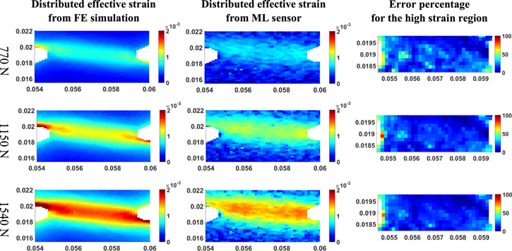
Figure 12. Distributions of the effective strains by the ML sensor and FE simulation of pure shear test in the zoomed-in region of interest with error percentages at different loading levels.
Download figure:
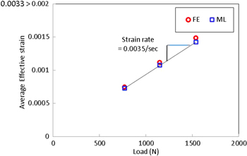
Standard image High-resolution imageThe applied load on the pure shear specimen versus averaged values of the effective strain from the ML sensor and FE simulation for the cropped region (see figure 12) is plotted in figure 13. The figure shows that the average value of the effective strain from ML sensor and FE simulation increase linearly by increasing the load level and the difference between them increases slightly at higher strain levels.
Figure 13. The average effective strain from ML sensor and FE simulation results in the cropped region versus applied loads.
Download figure:
Standard image High-resolution image
According to results from validation tests, errors were observed from comparing effective strains for ML sensor models and FEA. The sources for these errors could be listed as following:
- The measured effective strains are based on raw ML light intensities that may contain errors from environmental ambient light and camera noise.
- ML light emission is known to vary by temperature changes. Thus, the errors may be slightly influenced by changes of temperature. However, all the tests in this paper were conducted at room temperature. So, the temperature effect would be minimal.
- ML sensing film used in the reference tests could have concentrations and quality of dispersions of ML particles in the epoxy resin which are different from the ML sensing films used in validation experimental tests.
- ML sensing films used in the reference tests could have different thickness from those used in validation experimental tests due to different level of shrinkage and precipitation of ML particles after cured.
- Adhesive is the connector element between specimen and ML film. Every crack, micro-crack or bonding failure in the structure of adhesive could disconnect ML film from the specimen and cause differences between effective strain from ML and effective strain from FE.
Therefore, it is important to note that for an ML sensing film with a different thickness, concentration ratio or test conditions, the parameters of the proposed model may need to be recalibrated with new test data.
6. Conclusions
In this paper, quantitative full-field strains were measured for the first time by using ML thin film sensor made of SrAl2O4:Eu2+,Dy3+ (SAOED) particles and epoxy resin. For this purpose, two different standard reference tests were proposed to derive calibrated relationships of relative changes of ML light intensity with the effective strain: (1) uniaxial tensile reference test and (2) non-uniform strain reference test.
From each of the reference test methods, two calibration models for ML strain sensors were developed in a recurrence equation form to measure the full-field effective strain. Well-known strain rate effect on the ML light intensity was considered in the calibrated relationship by including the time step size  .
.
The verification of the calibrated effective strain values showed that these proposed calibration models can accurately measure the realistic strain values under various strains and strain rates. An open-hole test was conducted in order to validate the performance of the proposed calibration model from the uniaxial tensile reference test. The model from the non-uniform strain reference test was validated with the four-point bending test and pure shear test. For all of the experiments, the distributed effective strain values from ML sensor were compared with results from verified FE models. Strain and strain rates from the reference tests range from 0.0001 to 0.0033 and from 0.000 34 s−1 to 0.0025 s−1, respectively. The comparisons of the ML and the FE effective strain values clearly showed that the ML sensing film and the calibration models can be effectively used as a new non-contact full-field strain sensing methodology. A noticeable advantage of the proposed full-field strain measurement by ML sensor is its facet-free full-field strains with pixel-level resolutions. Moreover, the ML sensing film can be applied to a wide variety of materials (e.g. metals, concrete, composites, woods, plastics, etc) without limitations and are also cost-effective, less-hazardous and less-skillful. Therefore, the proposed full-field strain sensing method by ML sensor are expected to be widely used in various practical applications such as strain-based SHM/non-destructive testing (e.g. dynamic crack visualization) and experimental tests of critical structural components, etc. Another promising applications would be measurements of the applied loadings from ML sensors.
Although it is considered a promising sensing method, there are still challenges in improving its performance such as increasing its sensitivity to low and practical strain level, dynamic strain measurements, etc.
Acknowledgments
This research was supported by the Institute of Advanced Aerospace Technology at Seoul National University. Authors are grateful for their financial supports.