

Abstract
Objects sensed by laser interferometers are usually not stable in position or orientation. This angular instability can lead to a coupling of angular tilt to apparent longitudinal displacement—tilt-to-length coupling (TTL). In LISA this is a potential noise source for both the test mass interferometer and the long-arm interferometer. We have experimentally investigated TTL coupling in a setup representative for the LISA test mass interferometer and used this system to characterise two different imaging systems (a two-lens design and a four-lens design) both designed to minimise TTL coupling. We show that both imaging systems meet the LISA requirement of ±25 μm rad−1 for interfering beams with relative angles of up to ±300 μrad. Furthermore, we found a dependency of the TTL coupling on beam properties such as the waist size and location, which we characterised both theoretically and experimentally.
Export citation and abstract BibTeX RIS

Original content from this work may be used under the terms of the Creative Commons Attribution 3.0 licence. Any further distribution of this work must maintain attribution to the author(s) and the title of the work, journal citation and DOI.
1. Introduction
The space-based gravitational wave detector Laser Interferometer Space Antenna (LISA) [1, 2] has been selected as third large-class mission in ESA's science program [3]. LISA consists of three satellites forming an equilateral triangle with 2.5 million kilometres arm length. Laser beams are exchanged between satellites and the distance changes caused by gravitational waves between free-floating test masses inside the satellites are measured. Telescopes are used for sending and receiving light between spacecraft and the interferometric path length measurements are split in different parts. Each satellite has optical benches with several interferometers: the test mass interferometer measures distance changes between local test mass and optical bench. The long-arm interferometer measures distance changes between the local and the remote spacecraft. To detect gravitational waves these individual measurements are combined to form a Michelson-like interferometer. The freely-floating test masses and local interferometry have recently been demonstrated on the LISA Pathfinder (LPF) spacecraft [4, 5].
Cross-coupling from spacecraft motion into the longitudinal readout was an important noise source within LPF [6]. This tilt-to-length (TTL) coupling is also a significant contributor in LISA's noise budget. In addition, TTL coupling is also relevant for the laser ranging interferometer (LRI) onboard the GRACE follow-on (GFO) satellites [7].
Previously, TTL coupling was reduced in a proof-of-principle experiment by a two-lens imaging system [8]. The reference interferometer in this experiment was made insensitive to TTL coupling [9] by using a large single-element photo diode (SEPD) that fully detected the interference of identical Gaussian beams. In LISA, neither SEPDs can be used nor can the interfering beams be Gaussians with equal parameters.
In LPF the TTL coupling was characterised by intentionally inducing angular variations and measuring the system's response. With this knowledge the TTL coupling was subtracted in post-processing [6]. For LISA however, this procedure is not sufficient. Due to larger expected angular jitter and more stringed requirements additional measures are needed to reduce TTL coupling to a level that can be successfully subtracted in post-processing.
In LISA, TTL coupling is expected in the test mass interferometer due to spacecraft angular jitter relative to the beam reflected from the test mass and in the long-arm interferometer due to angular jitter between the beam received from the far spacecraft and jitter of the local spacecraft. Hence we built a test bed to experimentally investigate both cases. The test bed consists of two separate parts: an optical bench (OB) and a telescope simulator (TS). The OB simulates the relevant parts of the LISA optical bench and contains the measurement interferometer and the imaging systems under test. The TS is designed to deliver a phase stable, tilting beam (named Rx beam). The profile of the beam from the TS can be chosen to simulate either the LISA long-arm interferometer using a flat-top beam, or use a Gaussian beam to simulate the test mass interferometer.
The goal of this investigation is to experimentally demonstrate a reduction of TTL coupling in a setup representative for the LISA test mass interferometer to a coupling within ±25 μm rad−1 for angles within ±300 μrad between the interfering beams (this complies to ±1 pm / 40 nrad). This requirement comes from a top-level breakdown made in a previous mission study [10] that was adopted as a conservative and rather stringent requirement.
The test-setup used here is sketched in figure 1 and the more complex implementation is illustrated in figure 2. A detailed description of the test bed construction, why and how this is representative for LISA, fundamental measurement concepts, as well as the design of the two imaging systems characterised here is given in [11].

Figure 1. Schematic of the test bed concept. The telescope simulator (left) and optical bench (right) are shown with the key components to illustrate the measurement concept. The Rx beam is shown in green, the local oscillator (LO) beam in blue and the Tx beam in red. The Rx beam is tilted around the centre of the Rx clip with the two actuators. The beams between the two baseplates have a different polarization and are separated by polarizing beam splitters (PBS). Reproduced from [11]. © IOP Publishing Ltd. All rights reserved.
Download figure:
Standard image High-resolution image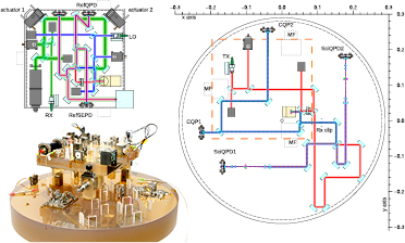
Figure 2. Optical layout of the test bed. For clarity, the TS (top left) is shown next to the OB (right). In the experiment, it is placed on top of the OB at the position marked with the dashed orange square with dedicated mounting feet (MF). A photo of the setup is shown bottom left, reproduced from [11]. © IOP Publishing Ltd. All rights reserved. The origin of the coordinate system is on the surface of the OB. The positive z axis points upwards (out of the paper plane). The TS can be adjusted in all three lateral degrees of freedom x, y, z and it can be rotated around all three axes. Rx beam: green, LO beam: blue, Tx beam: red.
Download figure:
Standard image High-resolution imageA summary of the measurement concepts used in the test-bed and the principle functions of the two imaging systems tested here, can be found in section 2. The preparation and characterisation of the laser beams, as well as alignment procedures and resulting alignment precisions of the test bed and its calibration, are given in section 3. The measured TTL suppression results and the dependency on beam parameters are presented in section 4.
2. Measurement concepts
2.1. Working principle of imaging systems
Two imaging system designs were tested: a four-lens system designed with classical concepts for pupil plane imaging, and a two-lens system which unlike the four-lens system generates a diverging output beam. Both imaging system types are designed to suppress the TTL coupling by imaging the point of rotation in the Rx clip to the quadrant photodiodes named SciQPD1 and SciQPD2. To avoid systematic errors, two identical copies of each imaging system design were manufactured, and one copy placed in front of each SciQPD. Each measurement was performed with both copies simultaneously in the two output ports. Details on the optical and mechanical imaging system designs, requirements, and specifications are given in [11].
2.2. Test bed summary
In the context of this paper, the aim of the test bed is to validate that TTL coupling, (i.e. the cross coupling of beam tilt caused by angular misalignment between test mass and optical bench to the interferometric phase) in a system representative for the LISA TM interferometer can be characterised and suppressed. In order to investigate this TTL coupling, the test bed does not feature a test mass (TM), but only a Gaussian beam (named here Rx beam, see figure 1) which rotates around a fixed point (labelled Rx clip) which represents the reflection point on the rotating TM. We then measure the TTL coupling between the tilting Rx beam and a fixed Gaussian reference beam named Tx beam on quadrant photodiodes (SciQPD1, SciQPD2) at distances behind the rotation point representative for the LISA OB and show that imaging systems reduce this coupling to below the given requirement.
In LISA the beam reflecting from the TM surface will be rotated, but not translated by TM angular jitter. Even TM lateral jitter [6] does not lead to a considerable amount of beam translation. In our measurement concept the Rx clip mimics the test mass position. We therefore require that the Rx beam rotates about he Rx clip, but that there is no lateral beam movement at the Rx clip during the beam rotation. We also require that the phase of the Rx beam relative to the Tx beam does not change during rotations induced by the actuators on the TS. The longitudinal requirement originates from the necessity to remove (or measure) any tilt dependent path length change that is induced up to the Rx clip.
In order to ensure these two requirements are met, the beam walk and the phase difference need to be monitored and controlled in the Rx clip. However, it is not possible to measure those quantities directly in the Rx clip without blocking the beam path to the SciQPDs. Therefore, a RefSEPD and a RefQPD are placed at positions equivalent to that of the Rx clip. With 'equivalent position' we mean, that a beam rotated around the centre of the RefQPD or RefSEPD also rotates around the centre of the Rx clip. We use the differential power sensing (DPS) signals [12] of the RefQPD to measure lateral displacement of the Rx beam in the Rx clip. The beam walk is then suppressed by nulling the DPS signal using actuator 2 (see figure 2). The longitudinal alignment of the rotation point is controlled by feeding the RefSEPD phase signals back to actuators on the modulation bench (path length stabilisation in figure 3), thereby locking the Tx and Rx beam to the local oscillator (LO) beam. This minimizes the phase variations between the beams in the location of the Rx clip. The method of fixing the centre of rotation in the Rx clip by phase locking the Rx and Tx to the LO beam on the RefSEPD is achieved by using a 150 μm diameter 'pinhole' aperture attached to the RefSEPD. A rotation of curved wavefronts around the centre of a larger diode would lead to TTL coupling [13]. The phase lock would then compensate the TTL coupling with a longitudinal shift of the Rx beam, inducing an unintended phase error in the Rx clip. For a pinhole diode the effective wavefront curvature with respect to the diodes size is negligible, such that the plane wave approximation is valid. The described effect was validated for the chosen pinhole size and the anticipated wavefronts using the simulation software IfoCAD [12]. Therefore, the phase lock on the pinhole RefSEPD ensures rotation of the Rx beam around the centre of the Rx clip.
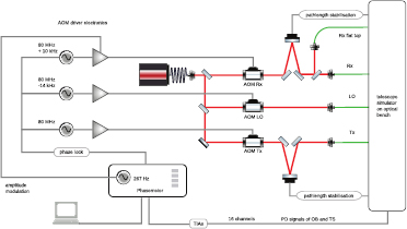
Figure 3. Schematic of laser preparation, electronics, and interferometer readout. Fibres: green, laser beams: red, cables: grey. The optical fibres are connected to the different fibre injectors of the test bed shown in figure 2. The transimpedance amplifiers (TIA) are connected to the photodiodes on the TS and OB shown in the same figure.
Download figure:
Standard image High-resolution imageAny residual phase variations that are not cancelled by this phase lock are subtracted from the SciQPDs signals in post processing.
Since the test bed is split into the TS and the OB, the described measurement principle naturally requires that these two parts are well aligned with respect to each other. This is achieved by aligning the LO beam to a pair of pre-aligned quadrant diodes (CQP1, CQP2 shown in figure 2). As described in [11] the LO beam is then optimally aligned to the SciQPDs and the TS is optimally aligned to the OB.
Details on the describes test bed methodology including alignment and calibration of the various subsystems are given in section 3. For instance, more details on the longitudinal positioning and lateral alignment of the RefSEPD and RefQPD to the equivalent position of the Rx clip is given in sections 3.6 and 3.7. Further details on the alignment of the TS to the OB are given in section 3.3.
3. Experiments
3.1. Laser preparation and beam characteristics
Figure 3 shows the schematic of laser preparation, electronics and the interferometer readout. The laser is a nonplanar ring oscillator [14, 15]. The beam is divided into three parts to generate the three different frequencies for the OB and TS. The frequency is shifted by acousto-optical modulators (AOMs), the frequency shifts and resulting heterodyne frequencies are listed in tables 1(a) and (b). The different heterodyne signals are called A, B and C in the following. They were chosen using the following criteria:
- They shall be of the form
 with k integer and the sampling frequency MHz of the phasemeter. This ensures that the heterodyne frequencies can be generated within the phasemeter.
 - Heterodyne frequencies B and C should be as high as possible to enable high bandwidth control loops.
- Heterodyne frequencies in the range of 10–30 kHz seemed to be sufficient.
- Heterodyne frequencies must not be harmonics of each other.
- Heterodyne frequencies must not be harmonics of the power grid frequency of 50 Hz.


Table 1. AOM and heterodyne frequencies.
| (a) AOM driving frequencies | |
|---|---|
| Beam | Frequency (MHz) |
| LO | 79.985 351 5625 |
| Tx | 80.0 |
| Rx | 80.009 765 625 |
| (b) Heterodyne frequencies | ||
|---|---|---|
| Phase | Beams | Frequency (kHz) |
| A | Tx-Rx | 9.765 6250 |
| B | Tx-LO | 14.648 4375 |
| C | Rx-LO | 24.414 0625 |
The three beams are delivered to the setup by optical fibres. Before the delivery to the test bed, the Rx beam is split again and coupled into two different fibres to allow an easy switching between a Gaussian and a flat-top shaped Rx beam. However, this work concentrates on the test mass interferometer, so the flat-top option is not used in the scope of this work.
In the beam path of the Tx and the Rx beams there are additional linear piezo actuators after the AOMs. They are used for optical pathlength stabilisations (phase lock between Tx, Rx and LO) implemented in the phasemeter, as previously described in section 2.2.
3.2. Beams
The beam parameter dependency of the TTL coupling, which will be described in detail in sections 4 and 5, generated a need to alter the Rx beam parameters. Therefore, we distinguish between the Rx beam delivered from the monolithically-bonded Rx fibre output coupler (labelled MBF) and the alternative Rx beam delivered by a gravity-mounted fibre output coupler (named GMF).
The MBF, silicate-bonded [16] to the TS, originally delivered the Rx beam. The GMF was designed to temporarily block the MBF and thereby easily alter the beam parameters of the Rx beam as shown in figure 4. The GMF consists of a commercially available fibre coupler (60FC-4-A15-03 by Schäfter+Kirchhoff) mounted in a brass mount with a folding mirror. The GMF could be placed and aligned 'by hand' on the TS because the two actuators could be used for the fine alignment of the Rx beam.
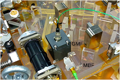
Figure 4. Rx beam delivery to the telescope simulator. It is shown how the MBF beam can be exchanged by the GMF beam.
Download figure:
Standard image High-resolution imageFigure 5 shows measured and fitted beam radii for MBF, Tx and GMF beams at different distances from the Rx clip. Plus signs indicate Gaussian beam radii obtained from fitting Gaussian intensity profiles to measured intensity distributions. Lines indicate equation (1) fitted to the measured beam radii with fit parameters w0 and z0. The shaded areas are the 95% confidence intervals for beam radii resulting from the respective confidence intervals for w0 and z0. For Gaussian beams, the beam radius w at position z is given by [17]

where w0 is the waist radius, z0 the location of the waist and  nm the laser wavelength. The MBF is from a different design than LO and Tx fibre couplers. In contrast to Tx and GMF, the intensity distributions of the MBF beam showed non-Gaussian contributions.
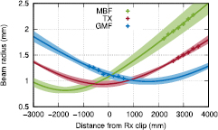
Figure 5. Beam radii for MBF, Tx and GMF beams as function of distance to the Rx clip; plus signs indicate Gaussian beam radii obtained from fitting Gaussian intensity profiles to measured intensity distributions, lines indicate equation (1) fitted to the measured beam radii with fit parameters w0 and z0. The shaded areas are the 95% confidence intervals for beam radii resulting from the respective confidence intervals for w0 and z0. Table 2 summarises the beam parameter values plotted here.
Download figure:
Standard image High-resolution imageThe GMF beam has a larger waist than the MBF beam. At position zero (at the Rx-clip) in figure 5 the curvatures of MBF and GMF have opposite sign. The imaging systems on the OB image the Rx beam at position zero (Rx clip) to the measurement QPDs. Hence, a change in the beam curvature at the Rx-clip also changes the beam curvature at the measurement interferometer QPDs.
Table 2 summarises the beam parameters plotted in figure 5. The table shows the waist radius and waist position along with the endpoints of the 95% confidence intervals. The listed waist position is given relative to the Rx clip. The positive direction points towards the measurement interferometers.
Table 2. Gaussian parameters of MBF, GMF, and Tx. Here, w0 and z0 are the waist radius and position, respectively. The indices 'min' and 'max' are the lower and upper endpoints of a 95% confidence interval. All values are given in mm.
| Beam | w0 |  |
 |
z0 |  |
 |
|---|---|---|---|---|---|---|
| MBF | 0.817 | 0.765 | 0.876 | −1714 | −1974 | −1473 |
| GMF | 0.989 | 0.932 | 1.044 | 1594 | 1361 | 1755 |
| Tx | 0.936 | 0.880 | 0.997 | −246 | −328 | −148 |
3.3. Telescope simulator alignment
As described in section 2.2 the TS is aligned with respect to the OB by centring the LO beam to the CQP diodes. For the x, y and yaw (around the z axis) degrees of freedom the TS is shifted in plane (see figure 2 for the definition of the coordinate system). For roll, pitch, and z degree of freedom (rotations around x, y, and z, respectively) the height of the individual mounting feet (see figure 2 and [11]) is adjusted. With this method the beam was centred on the CQP diodes with a 1–2 μm accuracy. This is sufficiently accurate and was limited by beam jitter due to air movement.
3.4. Tilt actuation of the Rx beam
In section 2.2 we described why the Rx beam needs to rotate around the Rx clip and the principle of how to achieve this. In the following, we describe the technical implementation of this concept.
The Rx beam was aligned to the LO beam and tilted around the centre of the Rx clip with the two piezo actuators on the TS by an automatic procedure that was implemented in the readout program. The procedure used the position of the Rx beam on the RefQPD on the TS and the angle between Rx and LO beam at the RefQPD. The Rx beam position on the RefQPD was obtained by a power modulation of the Rx beam at a frequency of 267 Hz imposed by the Rx AOM. Demodulation of the RefQPD signals in the phasemeter allowed the computation of differential power sensing (DPS) signals [12]. The calibrated DPS signals delivered the Rx beam position on the RefQPD. The beam angle between Rx and LO beams on the RefQPD was obtained from differential wavefront sensing (DWS) signals [18, 19].
The alignment procedure required that the Rx beam hit the RefQPD under a sufficiently small angle (<500 μrad) so that meaningful DWS signals could be computed. Typically, the angle between Rx beam and LO beam was aligned to better than 10 μrad and the centring of the Rx beam on the RefQPD was within 5 μm.
For a tilt-to-length coupling measurement, the Rx beam was aligned in both axes. Beam tilt was performed in the vertical axis (z-axis, see figure 2 for the definition of the coordinate system). Starting from angle zero, beam angle steps towards negative angles, from the most negative angle towards the most positive angle and finally towards zero were commanded. After each angle step, the Rx beam was centred on the RefQPD. This ensured that the beam was tilted around the RefQPD and hence around the Rx clip. For each of the 74 angle steps 90 s of data were averaged. The mean DWS signal between Rx and LO beam was used as measure for the Rx beam angle. Path length signals of all diodes were recorded. In the x-axis the Rx beam was not actively actuated. During all of the 74 angle steps, the centring of the Rx beam on the RefQPD stayed constant to within ±3 μm in both x and z axes. The angle in the x axis, which was not actively controlled, stayed constant within ±15 μrad.
3.5. Beam angle calibration
The aim of the given experiment is to demonstrate that the TTL coupling can be reduced to less than ±25 μm rad−1. Here, the angle given in radian is the tilt angle of the Rx beam relative to the LO beam. The DWS signal between Rx and LO (see phase C in table 1(a)) on the RefQPD is correlated to this relative beam angle. The parameters of this correlation are initially unknown and need to be calibrated. As described below, this is obtained here via the DPS signal on the CQPs, for both Rx beam implementations (MBF and GMF).
For each Rx beam, its position on CQP2 was measured along with the DWS signal on the RefQPD while the Rx angle was varied. In the second step, Rx beam angles were computed from the beam positions, plotted as function of DWS signal and the resulting graph was fitted by a third order polynomial. The DPS signal on CQP2 was calibrated via an analytical expression, which depends only on the diode's geometry and the spot size of the Rx beam [20]. The Rx spot size was taken from figure 5 at position 601.9 mm, which is equivalent to the CQP2 position relative to the Rx clip.
3.6. Reference interferometer longitudinal positioning
As described in section 2.2, the reference detectors (RefSEPD and RefQPD) need to be in positions equivalent to the Rx clip. Here, a millimetre longitudinal accuracy is sufficient [13]. This was achieved by sufficiently stringent manufacturing tolerances of the test bed and careful positioning of the Rx clip mount and the mount of the RefSEPD.
For the optical design, it is not the optical path length  that needs to be matched but
  , where ni is the refractive index and di the geometrical length of segment i. The quantity
  is also relevant for and known from the mode propagation of Gaussian laser beams and higher order modes.
3.7. Reference interferometer lateral alignment
After the longitudinal alignment, the RefSEPD also needs to be aligned laterally to the Rx clip. We do this by rotating the Rx beam while measuring the phase changes on the RefSEPD and in the Rx clip, thereby comparing the TTL coupling at these two positions. Any mismatch between these two points laterally to the LO beam axis leads to linear TTL coupling while longitudinal mismatch contributes quadratically. The differential TTL coupling in these two points was required to be less than ±25 μm rad−1.
The lateral alignment was achieved in a four-step procedure. The first step was already described in section 3.3 where the LO beam was aligned to the CQPs. This established the LO beam as a reference for temporary photo diodes in the Rx clip on the OB. In the second step, a QPD was placed temporarily in the Rx clip and aligned to the LO using DPS signals. In the third step the temporary QPD was replaced by a temporary SEPD (identical to the RefSEPD) such that the temporary SEPD was precisely centred to the temporary QPD (within a few micrometers). This temporary SEPD (TempSEPD) was thereby centred on the LO beam. In the fourth step, the RefSEPD was laterally aligned to the TempSEPD.
3.7.1. Alignment of the temporary diodes.
The co-alignment between temporary QPD and temporary SEPD was achieved with the help of the apertures shown in figure 6. The left aperture is attached to the temporary QPD, the right aperture is attached to the TempSEPD. The width and height of the apertures are 20 mm. The central holes are the defining apertures for the QPD and the SEPD with diameters of 0.5 mm and 0.15 mm, respectively. The apertures are laser-cut from 0.1 mm thick magnetic stainless steel foil (type AISI 430). They can be attached to three spherical magnets in the Rx clip via the rectangular slits. Then, the centre of the SEPD is at the centre of the four holes within a few micrometers.
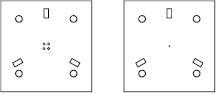
Figure 6. Apertures permanently fixed to the temporary photo diodes in the Rx clip. They can be attached to three spherical magnets in the Rx clip via the rectangular slits. Then, the centre of the SEPD is at the centre of the four holes within a few micrometers.
Download figure:
Standard image High-resolution image3.7.2. Lateral RefSEPD alignment procedure.
The lateral alignment of the RefSEPD has to be accurate to micrometer level and was achieved by measuring the TTL coupling difference of the two SEPDs (RefSEPD and TempSEPD).
The following alignment procedure was used
- (i)Measure the TTL coupling between Rx and LO on the RefSEPD and subtract this from the corresponding TTL coupling on the TempSEPD.
- (ii)If there is a difference move the RefSEPD laterally.
- (iii)Perform another TTL measurement.
- (iv)Repeat until the difference between the two SEPDs is minimized.
Figure 7 shows the difference of the path length signal between the RefSEPD and the TempSEPD in the Rx clip with the MBF beam after completion of the alignment procedure for the MBF beam. The linear coupling could be reduced to be well below the requirement of 25 μm rad−1 by aligning the RefSEPD laterally. The quadratic coupling that is still visible after the alignment cannot be reduced by a lateral alignment of the RefSEPD [13] but is sufficiently small to fulfil the requirement.
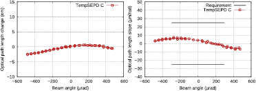
Figure 7. Difference of the path length signal between the RefSEPD and the TempSEPD in the Rx clip with the MBF beam. The RefSEPD is aligned to minimize the path length change. Left: Path length change versus beam angle, right: Slope of path length change versus beam angle.
Download figure:
Standard image High-resolution image3.8. Mitigation of temperature-driven length changes
The tip-tilt mount used for TS alignment was designed to be picometre-stable if required. For this reason the feet of the mount could be clamped to the telescope simulator and the vertical alignment screws could be retracted. The TS then had a connection to the OB entirely of low-expansion material (Zerodur by Schott for the TS baseplate and connection blocks and Ultra-Low Expansion (ULE) glass by Corning for the feet).
In our experiment we omitted clamping of the feet and retraction of the alignment screws because we did not require picometre stability and it allowed easier handling of the TS. Consequently, in some TTL measurements we observed temperature-driven drifts of the path length signals (see figure 8 and figure 9 in [11]). We believe these drifts to be dominated by the thermally-driven expansion of the alignment screws. We used a combination of measurement signals to remove this effect.
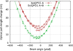
Figure 8. Path length change between SciQPD1 and RefSEPD plotted over the beam angle for a comparison between A phase and A + B phase. The traces have been vertically shifted for clarity. The A phase signal shows a drift that is removed in the A + B phase signal.
Download figure:
Standard image High-resolution imageThe height of the TS is measured in two phase signals: in signal A between Tx and Rx and in signal B between LO and Tx. Since the phase B measures the phase relation between two stable beams, it is a good measurement of the height variation of the TS. In the following we will use the B phase signal to correct for the height variations of the TS in the A phase. Thus we minimise our sensitivity to TS movement in the z direction.
Figure 8 shows a comparison between only A phase and A + B phase when no imaging system was present in the measurement interferometer. In the only A phase trace a drift can be observed which is caused by a height change of the TS. If the B phase is added, the drift disappears and the measured curve is not affected by the height variations any more.
In figure 8 and all following figures that use QPDs the phase signals of the four segments of each QPD are averaged (see equation (5) in [21]). From this average the phase signal of the RefSEPD is subtracted. The phase difference  is converted to an optical length change
  according to
  .
.
3.9. Alignment of photo diodes and imaging systems
Before the two imaging systems can be placed on the optical bench in their nominal position, they need to be assembled and pre-aligned. Therefore, the lenses (and lens pairs in the case of the four-lens imaging system) are held by adjustable mounts, fixed to a 'super baseplate' which can be attached to the OB.
For the pre-alignment of the two-lens imaging systems we used a QPD and a tiltable beam. We performed the alignment in two steps. In the first step lens 2 and later lens 1 were aligned on a centre beam at their nominal longitudinal positions. In the second alignment step a tilting beam was used. The beam walk on the QPD behind the imaging system was minimized by changing the distance between the lenses.
For the pre-alignment of the four-lens imaging systems we used a Shack-Hartmann sensor (SHS) with built-in light source and a double-pass configuration. In the alignment steps, we placed the imaging system in between SHS and a plane mirror and minimised wavefront errors. First, we aligned the lens pair L1 + L2, removed it from the super baseplate, rotated the super baseplate by 180° and inserted and aligned lens pair L3 + L4. Then we aligned the lens pairs to each other on the super baseplate.
After these steps, the imaging systems are pre-aligned and then need to be placed on the OB such that the Rx clip is imaged to the SciQPDs. That means, the SciQPDs sense no beam walk when the Rx beam is rotated around the Rx clip. In a classical imaging system the SciQPDs are thereby located in the exit pupil, while the Rx clip defines the entrance pupil.
3.10. Optimisation of the diode position
Placing the SciQPDs into the exit pupil does not necessarily define minimal TTL coupling. The point to point imaging ensures that there is no geometrical TTL coupling. That means, assuming a perfect imaging system and plane waves without clipping there is no TTL coupling on the SciQPDs. However, the use of Gaussian laser beams, imperfect imaging, and clipping on the QPDs' slits and outer borders result in a residual TTL coupling on the SciQPDs located in the exit pupil. As mentioned before and described in detail in [13], lateral (longitudinal) shifts of the diodes result in additional linear (quadratic) TTL coupling. Therefore, we shift the SciQPDs intentionally laterally to minimize any residual linear TTL coupling and longitudinally to reduce any residual quadratic TTL coupling. Effectively we thereby counteract the TTL coupling of the described non geometric sources with two geometric effects. In this work, we call the position with minimal TTL coupling 'optimal position'. All measurements shown in section 4 are performed with the SciQPDs in optimal position.
4. Results
4.1. Tilt-to-length coupling using the GMF beam
Figures 9 and 10 show the TTL coupling using the GMF behind the two-lens and four-lens imaging systems, respectively. The left side shows path length change versus beam angle, the right side shows the slope of path length change versus beam angle. For both SciQPDs and both imaging systems the path length slopes are well within the requirement. Since our aim was to show that TTL coupling in the measurement interferometer could be brought within the requirement using adequate imaging systems, no attempts were made to further reduce the TTL coupling or match the coupling of the two SciQPDs.

Figure 9. Two-lens imaging systems performance using the GMF beam; Both two-lens imaging systems fulfil the TTL requirement.
Download figure:
Standard image High-resolution image
Figure 10. Four-lens imaging systems performance using the GMF beam; Both four-lens imaging systems fulfil the TTL requirement.
Download figure:
Standard image High-resolution image4.2. Tilt-to-length coupling using the MBF beam
Figure 11 shows the TTL coupling behind the two-lens imaging systems using the MBF. For an Rx beam tilt of ±300 μrad a residual coupling of −30 μm rad−1–40 μm rad−1 was obtained, which is violating the requirement of ±25 μm rad−1. The same measurement with the four-lens imaging systems using the MBF beam is shown in figure 12. The residual TTL coupling was ±100 μm rad−1 at ±300 μrad Rx beam angle, clearly violating the requirement of ±25 μm rad−1.
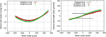
Figure 11. Two-lens imaging systems performance using the MBF beam; Changing the Rx beam (from the GMF) to the MBF leads to a violation of the requirement for both two-lens imaging systems.
Download figure:
Standard image High-resolution image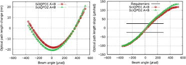
Figure 12. Four-lens imaging systems performance using the MBF beam; Changing the Rx beam (from the GMF) to the MBF leads to a violation of the requirement for both four-lens imaging systems.
Download figure:
Standard image High-resolution image4.3. Discussion
These measurements were performed at the optimal SciQPD positions (see section 3.10), such that the shown residual TTL coupling could not be reduced further.
We have shown, that both types of imaging systems violated the requirement of ±25 μm rad−1 for Rx beam tilts of ±300 μrad if the MBF beam is used, but perform according to the requirement if the GMF beam is used. The performance of the imaging systems therefore clearly depends on beam properties.
The underlying mechanisms resulting in the violation of the requirement while using the MBF are discussed in section 5.
5. Tilt-to-length coupling simulations
In order to analyse the dependency of the TTL suppression performance on beam properties, we performed computer simulations using the software IfoCAD [12]. The optical setup with the different imaging systems and the optimisation to minimise the TTL coupling by shifting the photo diode (see section 3.10) was simulated and the influence of different beam parameters to the residual TTL was computed.
5.1. Simulation algorithm
The goal of this simulation is to show the best possible TTL coupling behind an imaging system (best possible: optimal QPD position for minimal coupling) as a function of the beam parameters—Rx and Tx waist radius and position—to find correlations between the different properties. In detail, the simulation follows the algorithm shown here:
- (i)The simulation assumes a perfectly aligned imaging system (either the two-lens or the four-lens system), the point of rotation is at position zero and all lenses and the QPD are at their nominal positions.
- (ii)The TTL coupling for given beam parameters of the Tx and Rx beam is computed in the range ofrad–rad. The maximum in the optical path length slope in this range is called cTTL. The simulated setup is spherically symmetric so an extension of the angular range down to rad will produce identical results.
- (iii)The QPD is then placed in its optimal position, i.e. it is shifted longitudinally until the TTL coupling (cTTL) is minimised. The optimal position is labeled dQPD and the TTL coupling at this optimised QPD location is called copt.
- (iv)Next, the beam parameters of the Rx beam (waist radius and waist position) are varied and the corresponding optimised couplings copt and the optimal QPD positions dQPD are computed for all combinations in the range of mm to mm and z0 = −2m– m. The results are plotted in a heat map, where the x axis is the waist radius of the Rx beam, the y axis is the waist position of the Rx beam and the colour identifies the optimal coupling copt in μm rad−1 (e.g. one sub-plot of figure 15).
- (v)
- (vi)Finally, coloured crosses are placed in each sub-plot, illustrating the fitted parameters and confidence intervals for the MBF (green) and the GMF (purple) beam.


The simulations therefore did not include imperfections of the imaging systems, beam imperfections such as deviations from the fundamental Gaussian model, or phase changes from the misalignment of the RefSEPD. Furthermore, the optimisation of the photo diodes alignment was stopped in the experiment once the TTL couplings were within the requirement, which is not reflected in the given simulation. Accordingly, a match of the computed TTL coupling factors with those obtained experimentally is not envisaged. Instead, the simulation fully focuses on the impact of beam parameters to the resulting TTL coupling.
5.2. Results for the four-lens imaging system
Figure 13 shows the multi-plot for the TTL slope copt behind the four-lens imaging system.

Figure 13. Simulated TTL coupling copt of the four-lens imaging system obtained following the procedure described in section 5.1. This shows a significant TTL coupling for the MBF beam, while the TTL coupling using the GMF beam is negligible.
Download figure:
Standard image High-resolution imageFor the GMF the optimal TTL coupling is negligible and far below the requirement. In contrast, for the MBF the residual TTL coupling is in the order 10–20 μm rad−1. Thereby, the beam parameter dependency observed in the experiment is clearly reflected in this simulation.
Figure 14 shows the corresponding computed optimal QPD positions. For the GMF beam, this optimal QPD position is about 10 mm, that means the distance between imaging system and QPD was increased by about 10 mm with respect to the nominal position, resulting in the low TTL coupling shown in figure 13. For the MBF beam the optimal position was computed to be −1 mm. This value was defined in the simulation to be the closest position to the imaging system allowed for the QPD, limited by the mechanical lens mount. In theory, the coupling could be reduced further by shifting the QPD closer to the imaging system or even virtually into it. This shows, that for a full compensation of the non-geometrical coupling effects, the QPD would need to be shifted closer to the imaging system, which however is not possible due to geometrical constraints. Due to these constraints, the compensation was incomplete, resulting in the high TTL coupling in figure 13 and the observed violation of the requirement in the experiment.
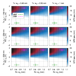
Figure 14. Optimal QPD position of the four-lens imaging system, corresponding to figure 13. This shows that when the MBF beam is used, the QPD is shifted by −1 mm, resulting in the closest possible distance behind the imaging system.
Download figure:
Standard image High-resolution image5.3. Results for the two-lens imaging system
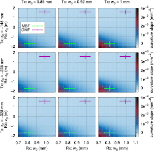
Figure 15 shows the multi-plot for the two-lens imaging system. Again, the TTL coupling is close to zero for the GMF beam and with about  m rad−1 significantly higher for the MBF beam. This value, however, is considerably smaller than observed in the corresponding experiment. The most likely explanation for this deviation is the focussing of the non-Gaussian contributions (mentioned in section 3.2) of the MBF beam in the two-lens imaging system.

Figure 15. Simulated TTL coupling copt of the two-lens imaging system. Again, a TTL coupling for the MBF beam can be observed, while this coupling is negligible if the GMF beam is used.
Download figure:
Standard image High-resolution imageIn figure 16 the optimal QPD position for the two-lens imaging system is shown, again as a function of the Tx and Rx parameters.
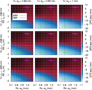
Figure 16. Optimal QPD position of the two-lens imaging system, corresponding to figure 15. The QPD positions ranging between −20 to +10 mm are not restricted by the experimental setup.
Download figure:
Standard image High-resolution imageFor the two-lens imaging system the reason for this behaviour is not the limited QPD shifting range as for the four-lens imaging systems. All optimal photo diode positions are well within the available range.
We know, that the TTL coupling depends on the difference of the wavefront curvature of the interfering beams. In the case of the four-lens system, the output beams are collimated (defined here by a maximal Rayleigh range). That means the curvature difference does not change over the available QPD shifting range. The two-lens system however, generates diverging output beams, such that the curvature difference depends on the QPD position. The curvature difference slope  defined as

describes this position dependency, with  and
and  being the curvatures of the Rx and the Tx wavefronts, dtmp is the longitudinal position of the QPD and dQPD is the optimal position of the QPD with minimal TTL coupling. This curvature difference is plotted in figure 17 and shows a clear correlation to the TTL coupling plotted in figure 15. This correlation and the non-negligible TTL coupling in the two-lens imaging system using the MBF beam can probably be explained as follows. As described in section 3.10, the aim is to null the quadratic TTL coupling originating from various non-geometric effects by an additional quadratic coupling induced by longitudinally shifting the QPD. While shifting the QPD, a curvature slope generates an additional quadratic coupling. With the beam parameters of the MBF the curvature slope coupling counteracts the coupling induced by the QPD shift. Consequently, is not possible to null the quadratic TTL coupling from other non-geometric effects by changing the longitudinal position of the photo diode.
Figure 17. Simulated beam curvature difference slope at the optimal QPD position behind the two-lens imaging system, corresponding to figure 15. A clear correlation between the TTL coupling and the curvature difference slope can be observed.
Download figure:
Standard image High-resolution image
6. Conclusion
We have demonstrated the use of imaging systems to minimise tilt-to-length (TTL) coupling in a setup representative for the LISA test mass interferometer. That means, we have shown experimentally for a two-lens and a four-lens imaging system that the TTL coupling could be reduced below the required ±25 μm rad−1 for angles within ±300 μrad between the interfering beams. We observed a beam parameter dependent performance of the imaging systems. This dependency was modelled numerically and explained. This shows additionally, that the TTL suppression of imaging systems can be modelled and predicted by numerical simulations.
Acknowledgments
We acknowledge funding by the European Space Agency within the project Optical Bench Development for LISA (22331/09/NL/HB), support from UK Space Agency, University of Glasgow, Scottish Universities Physics Alliance (SUPA), and support by Deutsches Zentrum für Luft und Raumfahrt (DLR) with funding from the Bundesministerium für Wirtschaft und Technologie (DLR project reference 50 OQ 0601). We thank the German Research Foundation for funding the cluster of Excellence QUEST—Centre for Quantum Engineering and Space-Time Research. Advanced imaging systems for future gravity missions were investigated in the frame of SFB1128 geo-Q and the dependency on beam parameters shown here was found. The simulations described in section 5 show results found within geo-Q project A05, adapted to the LISA imaging systems. We therefore gratefully acknowledge Deutsche Forschungsgemeinschaft (DFG) for funding geo-Q.