Abstract
For  a bounded domain in
  and a given smooth function
  , we consider the statistical nonlinear inverse problem of recovering the conductivity f > 0 in the divergence form equation
  from N discrete noisy point evaluations of the solution u = uf on
  . We study the statistical performance of Bayesian nonparametric procedures based on a flexible class of Gaussian (or hierarchical Gaussian) process priors, whose implementation is feasible by MCMC methods. We show that, as the number N of measurements increases, the resulting posterior distributions concentrate around the true parameter generating the data, and derive a convergence rate N−λ, λ > 0, for the reconstruction error of the associated posterior means, in
  -distance.
Export citation and abstract BibTeX RIS

Content from this work may be used under the terms of the Creative Commons Attribution 4.0 licence. Any further distribution of this work must maintain attribution to the author(s) and the title of the work, journal citation and DOI.
1. Introduction
Statistical inverse problems arise naturally in many applications in physics, imaging, tomography, and generally in engineering and throughout the sciences. A prototypical example involves a domain  , some function
  of interest, and indirect measurements G(f) of f, where G is a given solution (or 'forward') operator of some partial differential equation (PDE) governed by the unknown coefficient f. A natural statistical observational model postulates data

where the Xi's are design points at which the PDE solution G(f) is measured, and where the Wi's are standard Gaussian noise variables scaled by a noise level σ > 0. The aim is then to infer f from the data  . The study of problems of this type has a long history in applied mathematics, see the monographs (Engl et al 1996, Kaltenbacher et al 2008), although explicit statistical noise models have been considered only more recently (Bissantz et al 2004, Bissantz et al 2007, Hohage and Pricop 2008, Kaipio and Somersalo 2004). Recent survey articles on the subject are (Arridge et al 2019, Benning and Burger 2018) where many more references can be found.
For many of the most natural PDEs—such as the divergence form elliptic equation (2) considered below—the resulting maps G are non-linear in f, and this poses various challenges: among other things, the negative log-likelihood function associated to the model (1), which equals the least squares criterion (see (10) below for details), is then possibly non-convex, and commonly used statistical algorithms (such as maximum likelihood estimators, Tikhonov regularisers or MAP estimates) defined as optimisers in f of likelihood-based objective functions can not reliably be computed by standard convex optimisation techniques. While iterative optimisation methods (such as Landweber iteration) may overcome such challenges (Kaltenbacher et al 2008, Hanke et al 1995, Kaltenbacher et al 2009, Qi-nian 2000), an attractive alternative methodology arises from the Bayesian approach to inverse problems advocated in an influential paper by Stuart (Stuart 2010): one starts from a Gaussian process prior Π for the parameter f or in fact, as is often necessary, for a suitable vector-space valued re-parameterisation F of f. One then uses Bayes' theorem to infer the best posterior guess for f given data  . Posterior distributions and their expected values can be approximately computed via Markov chain Monte Carlo (MCMC) methods (see, for example, Beskos et al 2017, Conrad et al 2016, Cotter et al 2013 and references therein) as soon as the forward map G(⋅) can be evaluated numerically, avoiding optimisation algorithms as well as the use of (potentially tedious, or non-existent) inversion formulas for G−1; see subsection 2.3.1 below for more discussion. The Bayesian approach has been particularly popular in application areas as it does not only deliver an estimator for the unknown parameter f but simultaneously provides uncertainty quantification methodology for the recovery algorithm via the probability distribution of
  (see, for example, Dashti and Stuart 2016). Conceptually related is the area of 'probabilistic numerics' (Briol et al 2019) in the noise-less case σ = 0, with key ideas dating back to work by Diaconis (1988).
As successful as this approach may have proved to be in algorithmic practice, for the case when the forward map G is non-linear we currently only have a limited understanding of the statistical validity of such Bayesian inversion methods. By validity we mean here statistical guarantees for convergence of natural Bayesian estimators such as the posterior mean ![$\overline{f}={E}^{{\Pi}}\left[f\vert {\left({Y}_{i},{X}_{i}\right)}_{i=1}^{N}\right]$](https://content.cld.iop.org/journals/0266-5611/36/8/085001/revision2/ipab7d2aieqn12.gif) towards the ground truth f0 generating the data. Without such guarantees, the interpretation of posterior based inferences remains vague: the randomness of the prior may have propagated into the posterior in a way that does not 'wash out' even when very informative data is available (e.g., small noise variance and/or large sample size N), rendering Bayesian methods potentially ambiguous for the purposes of valid statistical inference and uncertainty quantification.
towards the ground truth f0 generating the data. Without such guarantees, the interpretation of posterior based inferences remains vague: the randomness of the prior may have propagated into the posterior in a way that does not 'wash out' even when very informative data is available (e.g., small noise variance and/or large sample size N), rendering Bayesian methods potentially ambiguous for the purposes of valid statistical inference and uncertainty quantification.
In the present article we attempt to advance our understanding of this problem area in the context of the following basic but representative example for a non-linear inverse problem: let g be a given smooth 'source' function, and let  be a an unknown conductivity parameter determining solutions u = uf of the PDE

where we denote by ∇⋅ the divergence and by ∇ the gradient operator, respectively. Under mild regularity conditions on f, and assuming that f ⩾ Kmin > 0 on  , standard elliptic theory implies that (2) has a unique classical C2-solution G(f) ≡ uf. Identification of f from an observed solution uf of this PDE has been considered in a large number of articles both in the applied mathematics and statistics communities—we mention here (Stuart 2010, Beskos et al 2017, Dashti and Stuart 2016, Briol et al 2019, Alessandrini 1986, Bonito et al 2017, Dashti and Stuart 2011, Falk 1983, Hoffmann and Sprekels 1985, Ito and Kunisch 1994, Knowles 2001, Kohn and Lowe 1988, Kravaris and Seinfeld 1985, Nickl et al 2020, Richter 1981, Schwab and Stuart 2012, Vollmer 2013) and the many references therein.
The main contributions of this article are as follows: we show that posterior means arising from a large class of Gaussian (or conditionally Gaussian) process priors for f provide statistically consistent recovery (with explicit polynomial convergence rates as the number N of measurements increases) of the unknown parameter f in (2) from data in (1). While we employ the theory of posterior contraction from Bayesian non-parametric statistics (Ghosal and van der Vaart 2017, van der Vaart and van Zanten 2008, van der Vaart and van Zanten 2009), the non-linear nature of the problem at hand leads to substantial additional challenges arising from the fact that (a) the Hellinger distance induced by the statistical experiment is not naturally compatible with relevant distances on the actual parameter f and that (b) the 'push-forward' prior induced on the information-theoretically relevant regression functions G(f) is non-explicit (in particular, non-Gaussian) due to the non-linearity of the map G. Our proofs apply recent ideas from Monard et al (2020) to the present elliptic situation. In the first step we show that the posterior distributions arising from the priors considered (optimally) solve the PDE-constrained regression problem of inferring G(f) from data (1). Such results can then be combined with a suitable 'stability estimate' for the inverse map G−1 to show that, for large sample size N, the posterior distributions concentrate around the true parameter generating the data at a convergence rate N−λ for some λ > 0. We ultimately deduce the same rate of consistency for the posterior mean from quantitative uniform integrability arguments.
The first results we obtain apply to a large class of 'rescaled' Gaussian process priors similar to those considered in Monard et al (2020), addressing the need for additional a priori regularisation of the posterior distribution in order to tame non-linear effects of the 'forward map'. This rescaling of the Gaussian process depends on sample size N. From a non-asymptotic point of view this just reflects an adjustment of the covariance operator of the prior, but following Diaconis (1988) one may wonder whether a 'fully Bayesian' solution of this non-linear inverse problem, based on a prior that does not depend on N, is also possible. We show indeed that a hierarchical prior that randomises a finite truncation point in the Karhunen–Loéve-type series expansion of the Gaussian base prior will also result in consistent recovery of the conductivity parameter f in equation (2) from data (1), at least if f is smooth enough.
Let us finally discuss some related literature on statistical guarantees for Bayesian inversion: to the best of our knowledge, the only previous paper concerned with (frequentist) consistency of Bayesian inversion in the elliptic PDE (2) is by Vollmer (2013). The proofs in Vollmer (2013) share a similar general idea in that they rely on a preliminary treatment of the associated regression problem for G(f), which is then combined with a suitable stability estimate for G−1. However, the convergence rates obtained in Vollmer (2013) are only implicitly given and sub-optimal, also (unlike ours) for 'prediction risk' in the PDE-constrained regression problem. Moreover, when specialised to the concrete non-linear elliptic problem (2) considered here, the results in section 4 in Vollmer (2013) only hold for priors with bounded Cβ-norms, such as 'uniform wavelet type priors', similar to the ones used in Nickl (2018), Nickl and Söhl (2017), and Nickl and Söhl (2019) for different non-linear inverse problems. In contrast, our results hold for the more practical Gaussian process priors which are commonly used in applications, and which permit the use of tailor-made MCMC methodology—such as the pCN algorithm discussed in subsection 2.3.1—for computation.
The results obtained in Nickl et al (2020) for the maximum a posteriori (MAP) estimates associated to the priors studied here are closely related to our findings in several ways. Ultimately the proof methods in Nickl et al (2020) are, however, based on variational methods and hence entirely different from the Bayesian ideas underlying our results. Moreover, the MAP estimates in Nickl et al (2020) are difficult to compute due to the lack of convexity of the forward map, whereas posterior means arising from Gaussian process priors admit explicit computational guarantees, see Hairer et al (2014) and also subsection 2.3.1 for more details.
It is further of interest to compare our results to those recently obtained in Abraham and Nickl (2019), where the statistical version of the Caldéron problem is studied. There the 'Dirichlet-to-Neumann map' of solutions to the PDE (2) is observed, corrupted by appropriate Gaussian matrix noise. In this case, as only boundary measurements of uf at  are available, the statistical convergence rates are only of order log−γ(N) for some γ > 0 (as N → ∞), whereas our results show that when interior measurements of uf are available throughout
  , the recovery rates improve to N−λ for some λ > 0.
There is of course a large literature on consistency of Bayesian linear inverse problems with Gaussian priors, we only mention Agapiou et al (2013), Kekkonen et al (2016), Knapik et al (2011), Monard et al (2019), and Ray (2013) and references therein. The non-linear case considered here is fundamentally more challenging and cannot be treated by the techniques from these papers—however, some of the general theory we develop in the appendix provides novel proof methods also for the linear setting.
This paper is structured as follows. Section 2 contains all the main results for the inverse problem arising with the PDE model (2). The proofs, which also include some theory for general non-linear inverse problems that is of independent interest, are given in section 3 and appendix
2. Main results
2.1. A statistical inverse problem with elliptic PDEs
2.1.1. Main notation
Throughout the paper,  , is a given nonempty open and bounded set with smooth boundary
  and closure
  .
.
The spaces of continuous functions defined on  and
and  are respectively denoted
  and
and  , and endowed with the supremum norm ||⋅||∞. For positive integers
  ,
,  is the space of β-times differentiable functions with uniformly continuous derivatives; for non-integer β > 0,
  is defined as
where ⌊β⌋ denotes the largest integer less than or equal to β, and for any multi-index i = (i1, ..., id), Di is the ith partial differential operator.  is normed by
where the second summand is removed for integer β. We denote by  the set of smooth functions, and by
  the subspace of elements in
  with compact support contained in
  .
.
Denote by  the Hilbert space of square integrable functions on
  , equipped with its usual inner product
  . For integer α ⩾ 0, the order-α Sobolev space on
  is the separable Hilbert space
For non-integer α ⩾ 0,  can be defined by interpolation, for example, Lions and Magenes (1972). For any α ⩾ 0,
  will denote the completion of
  with respect to the norm
  . Finally, if K is a nonempty compact subset of
  , we denote by
  the closed subspace of functions in
  with support contained in K. Whenever there is no risk of confusion, we will omit the reference to the underlying domain
  .
.
Throughout, we use the symbols ≲ and ≳ for inequalities holding up to a universal constant. Also, for two real sequences (aN) and (bN), we say that aN ≃ bN if both aN ≲ bN and bN ≲ aN for all N large enough. For a sequence of random variables ZN we write ZN = OPr(aN) if for all ɛ > 0 there exists Mɛ < ∞ such that for all N large enough, Pr(|ZN| ⩾ MɛaN) < ɛ. Finally, we will denote by  the law of a random variable Z.
2.1.2. Parameter spaces and link functions
Let  be an arbitrary source function, which will be regarded as fixed throughout. For
  , consider the boundary value problem

If we assume that f ⩾ Kmin > 0 on  , then standard elliptic theory (e.g. Gilbarg and Trudinger (1998)) implies that (3) has a classical solution
  .
.
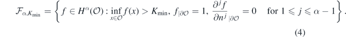
We consider the following parameter space for f: for integer α > 1 + d/2, Kmin ∈ (0, 1), and denoting by n = n(x) the outward pointing normal at  , let
, let
Our approach will be to place a prior probability measure on the unknown conductivity f and base our inference on the posterior distribution of f given noisy observations of G(f), via Bayes' theorem. It is of interest to use Gaussian process priors. Such probability measures are naturally supported in linear spaces (in our case  ) and we now introduce a bijective re-parametrisation so that the prior for f is supported in the relevant parameter space
  . We follow the approach of using regular link functions Φ as in Nickl et al (2020).
Condition 1. For given Kmin > 0, let  be a smooth, strictly increasing bijective function such that Φ(0) = 1,
  , and assume that all derivatives of Φ are bounded on
  .
.
For some of the results to follow it will prove convenient to slightly strengthen the previous condition.
Condition 2. Let Φ be as in condition 1, and assume furthermore that Φ' is nondecreasing and that lim inft→−∞Φ'(t)ta > 0 for some a > 0.
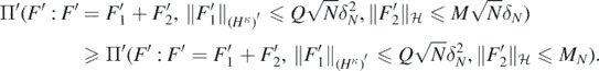
For a = 2, an example of such a link function is given in example 24 below. Note however that the choice of Φ = exp is not permitted in either condition.
Given any link function Φ satisfying condition 1, one can show (cf. Nickl et al (2020), section 3.1) that the set  in (4) can be realised as the family of composition maps

We then regard the solution map associated to (3) as one defined on  via
via

where G(Φ◦F) is the solution to (3) now with  . In the results to follow, we will implicitly assume a link function Φ to be given and fixed, and understand the re-parametrised solution map
  as being defined as in (5) for such choice of Φ.
2.1.3. Measurement model
Define the uniform distribution on  by
by  , where dx is the Lebesgue measure and
  , and consider random design variables

For unknown  , we model the statistical errors under which we observe the corresponding measurements
  by i.i.d. Gaussian random variables Wi ∼ N(0, 1), all independent of the Xi's. Using the re-parameterisation f = Φ◦F via a given link function from the previous subsection, the observation scheme is then

where σ > 0 is the noise amplitude. We will often use the shorthand notation  , with analogous definitions for X(N) and W(N). The random vectors (Yi, Xi) on
  are then i.i.d with laws denoted as
  . Writing dy for the Lebesgue measure on
  , it follows that
  has Radon–Nikodym density

We will write  for the joint law of (Y(N), X(N)) on
  , with
  ,
,  the expectation operators corresponding to the laws
  ,
,  respectively. In the sequel we sometimes use the notation
  instead of
  when convenient.
2.1.4. The Bayesian approach
In the Bayesian approach one models the parameter  by a Borel probability measure Π supported in the Banach space
  . Since the map (F, (y, x)) ↦ pF(y, x) can be shown to be jointly measurable, the posterior distribution Π(⋅|Y(N), X(N)) of F|(Y(N), X(N)) arising from data in model (7) equals, by Bayes' formula (p 7, Ghosal and van der Vaart 2017),

where

is (up to an additive constant) the joint log-likelihood function.
2.2. Statistical convergence rates
In this section we will show that the posterior distribution arising from certain priors concentrates near any sufficiently regular ground truth F0 (or, equivalently, f0), and provide a bound on the rate of this contraction, assuming the observation (Y(N), X(N)) to be generated through model (7) of law  . We will regard σ > 0 as a fixed and known constant; in practice it may be replaced by the estimated sample variance of the Yi's.
The priors we will consider are built around a Gaussian process base prior Π', but to deal with the non-linearity of the inverse problem, some additional regularisation will be required. We first show how this can be done by an N-dependent 'rescaling' step as suggested in Monard et al (2020). We then further show that a randomised truncation of a Karhunen–Loeve-type series expansion of the base prior also leads to a consistent, 'fully Bayesian' solution of this inverse problem.
2.2.1. Results with re-scaled Gaussian priors
We will freely use terminology from the basic theory of Gaussian processes and measures, see, for example, Giné and Nickl (2016), chapter 2 for details.
Condition 3. Let α > 1 + d/2, β ⩾ 1, and let  be a Hilbert space continuously imbedded into
  . Let Π' be a centred Gaussian Borel probability measure on the Banach space
  that is supported on a separable measurable linear subspace of
  , and assume that the reproducing-kernel Hilbert space (RKHS) of Π' equals
  .
.
As a basic example of a Gaussian base prior Π' satisfying condition 3, consider a Whittle–Matérn process  indexed by
  and of regularity α (cf. example 25 below for full details). We will assume that it is known that
  is supported inside a given compact subset K of the domain
  , and fix any smooth cut-off function
  such that χ = 1 on K. Then,
  is supported on the separable linear subspace
  of
of  for any β < β' < α − d/2, and its RKHS
  is continuously imbedded into
  (and contains
  ). The condition
  that is employed in the following theorems then amounts to the standard assumption that
  be supported in a strict subset K of
  .
.
To proceed, if Π' is as above and F' ∼ Π', we consider the 're-scaled' prior

Then ΠN again defines a centred Gaussian prior on  , and a basic calculation (e.g., exercise 2.6.5 in Giné and Nickl (2016)) shows that its RKHS
  is still given by
  but now with norm

Our first result shows that the posterior contracts towards F0 in 'prediction'-risk at rate N−(α+1)/(2α+2+d) and that, moreover, the posterior draws possess a bound on their Cβ-norm with overwhelming frequentist probability.
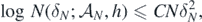
Theorem 4. For fixed integer α > β + d/2, β ⩾ 1, consider the Gaussian prior ΠN in (11) with base prior F' ∼ Π' satisfying condition 3 for RKHS  . Let ΠN(⋅|Y(N), X(N)) be the resulting posterior distribution arising from observations (Y(N), X(N)) in (7), set δN = N−(α+1)/(2α+2+d), and assume
  .
.
Then for any D > 0 there exists L > 0 large enough (depending on σ, F0, D, α, β, as well as on  ) such that, as N → ∞,

and for sufficiently large M > 0 (depending on σ, D, α, β)

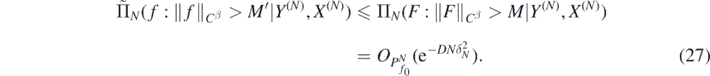
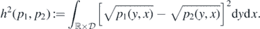
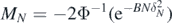
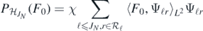
Following ideas in Monard et al (2020), we can combine (13) with the regularisation property (14) and a suitable stability estimate for G−1 to show that the posterior contracts about f0 also in L2-risk. We shall employ the stability estimate proved in Nickl et al (2020), lemma 24, which requires the source function g in the base PDE (3) to be strictly positive, a natural condition ensuring injectivity of the map f ↦ G(f), see Richter (1981). Denote the push-forward posterior on the conductivities f by

Theorem 5. Let ΠN(⋅|Y(N), X(N)), δN and F0 be as in theorem 4 for integer β > 1. Let f0 = Φ◦F0 and assume in addition that  . Then for any D > 0 there exists L > 0 large enough (depending on
  , gmin, d) such that, as N → ∞,

We note that as the smoothness α of f0 increases, we can employ priors of higher regularity α, β. In particular, if F0 ∈ C∞ = ∩α>0Hα, we can let the above rate N−λ be as closed as desired to the 'parametric' rate N−1/2.
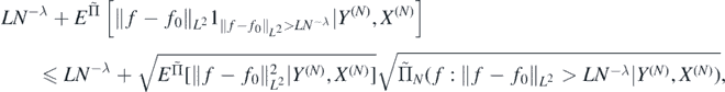
We conclude this section showing that the posterior mean EΠ[F|Y(N), X(N)] of ΠN(⋅|Y(N), X(N)) converges to F0 at the rate N−λ from theorem 5. We formulate this result at the level of the vector space valued parameter F (instead of for conductivities f), as the most commonly used MCMC algorithms (such as pCN, see subsection 2.3.1) target the posterior distribution of F.
Theorem 6. Under the hypotheses of theorem 5, let ![${\overline{F}}_{N}={E}^{{\Pi}}\left[F\vert {Y}^{\left(N\right)},{X}^{\left(N\right)}\right]$](https://content.cld.iop.org/journals/0266-5611/36/8/085001/revision2/ipab7d2aieqn107.gif) be the (Bochner-)mean of ΠN(⋅|Y(N), X(N)). Then, as N → ∞,
be the (Bochner-)mean of ΠN(⋅|Y(N), X(N)). Then, as N → ∞,

The same result holds for the implied conductivities, that is, for  replacing
  , since composition with Φ is Lipschitz.
2.2.2. Extension to high-dimensional Gaussian sieve priors
It is often convenient, for instance for computational reasons as discussed in subsection 2.3.1, to employ 'sieve'-priors that are concentrated on a finite-dimensional approximation of the parameter space supporting the prior. For example a truncated Karhunen–Loeve-type series expansion (or some other discretisation) of the Gaussian base prior Π' is frequently used (Dashti and Stuart 2011, Hairer et al 2014). The theorems of the previous subsection remain valid if the approximation spaces are appropriately chosen.
Let us illustrate this by considering a Gaussian series prior based on an orthonormal basis  of
of  composed of sufficiently regular, compactly supported Daubechies wavelets (see chapter 4 in Giné and Nickl (2016) for details). We assume that
  for some
  , and denote by
  the set of indices r for which the support of Ψℓr intersects K. Fix any compact
  such that K ⊊ K', and a cut-off function
  such that χ = 1 on K'. For any real α > 1 + d/2, consider the prior Π'J arising as the law of the Gaussian random sum

where J = JN → ∞ is a (deterministic) truncation point to be chosen. Then Π'J defines a centred Gaussian prior that is supported on the finite-dimensional space

Proposition 7. Consider a prior ΠN as in (11) where now F' ∼ Π'J and  is such that 2J ≃ N1/(2α+2+d). Let ΠN(⋅|Y(N), X(N)) be the resulting posterior distribution arising from observations (Y(N), X(N)) in (7), and assume
  . Then the conclusions of theorems 4–6 remain valid (under the respective hypotheses on α, β, g).
A similar result could be proved for more general Gaussian priors (not of wavelet type), but we refrain from giving these extensions here.
2.2.3. Randomly truncated Gaussian series priors
In this section we show that instead of rescaling Gaussian base priors Π', Π'J in an N-dependent way to attain extra regularisation, one may also randomise the dimensionality parameter J in (17) by a hyper-prior with suitable tail behaviour. While this is computationally somewhat more expensive (by necessitating a hierarchical sampling method, see subsection 2.3.1), it gives a possibly more principled approach to ('fully') Bayesian regularisation in our inverse problem. The theorem below will show that such a procedure is consistent in the frequentist sense, at least for smooth enough F0.
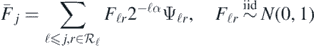
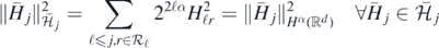
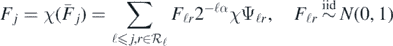
For the wavelet basis and cut-off function χ introduced before (17), we consider again a random (conditionally Gaussian) sum

where now J is a random truncation level, independent of the random coefficients Fℓr, satisfying the following inequalities:

When d = 1, a (log-)Poisson random variable satisfies these tail conditions, and for d > 1 such a random variable J can be easily constructed too—see example 28 below.
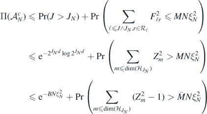
Our first result in this section shows that the posterior arising from the truncated series prior in (19) achieves (up to a log-factor) the same contraction rate in L2-prediction risk as the one obtained in theorem 4. Moreover, as is expected in light of the results in van der Vaart and van Zanten (2009) and Ray (2013), the posterior adapts to the unknown regularity α0 of F0 when it exceeds the base smoothness level α.
Theorem 8. For any α > 1 + d/2, let Π be the random series prior in (19), and let Π(⋅|Y(N), X(N)) be the resulting posterior distribution arising from observations (Y(N), X(N)) in (7). Then, for each α0 ⩾ α and any  , we have that for any D > 0 there exists L > 0 large enough (depending on
  ) such that, as N → ∞,

where  . Moreover, for
  the finite-dimensional subspaces in (18) and
  such that
  , we also have that for sufficiently large M > 0 (depending on D, α)

We can now exploit the previous result along with the finite-dimensional support of the posterior and again the stability estimate from Nickl et al (2020) to obtain the following consistency theorem for  if α0 is large enough (with a precise bound α0 ⩾ α* given in the proof of lemma 12).
Theorem 9. Let the link function Φ in the definition (5) of  satisfy condition 2. Let Π(⋅|Y(N), X(N)), ξN be as in theorem 8, assume in addition g ⩾ gmin > 0 on
  , and let
  be the posterior distribution of f as in (15). Then for f0 = Φ◦F0 with
  for α0 large enough (depending on α, d, a) and for any D > 0 there exists L > 0 large enough (depending on
  ) such that, as N → ∞,

Just as before, for f0 ∈ C∞ the above rate can be made as close as desired to N−1/2 by choosing α large enough. Moreover, the last contraction theorem also translates into a convergence result for the posterior mean of F.
Theorem 10. Under the hypotheses of theorem 9, let ![${\overline{F}}_{N}={E}^{{\Pi}}\left[F\vert {Y}^{\left(N\right)},{X}^{\left(N\right)}\right]$](https://content.cld.iop.org/journals/0266-5611/36/8/085001/revision2/ipab7d2aieqn131.gif) be the mean of Π(⋅|Y(N), X(N)). Then, as N → ∞,
be the mean of Π(⋅|Y(N), X(N)). Then, as N → ∞,

We note that the proof of the last two theorems crucially takes advantage of the 'non-symmetric' and 'non-exponential' nature of the stability estimate from Nickl et al (2020), and may not hold in other non-linear inverse problems where such an estimate may not be available (e.g., as in Monard et al (2020), Abraham and Nickl (2020) or also in the Schrödinger equation setting studied in Nickl et al (2020), Nickl (2018)).
Let us conclude this section by noting that hierarchical priors such as the one studied here are usually devised to 'adapt to unknown' smoothness α0 of F0, see van der Vaart and van Zanten (2009) and Ray (2013). Note that while our posterior distribution is adaptive to α0 in the 'prediction risk' setting of theorem 8, the rate N−ρ obtained in theorems 9 and 10 for the inverse problem does depend on the minimal smoothness α, and is therefore not adaptive. Nevertheless, this hierarchical prior gives an example of a fully Bayesian, consistent solution of our inverse problem.
2.3. Concluding discussion
2.3.1. Posterior computation
As mentioned in the introduction, in the context of the elliptic inverse problem considered in the present paper, posterior distributions arising from Gaussian process priors such as those above can be computed by MCMC algorithms, see Beskos et al (2017), Conrad et al (2016), Cotter et al (2013), and computational guarantees can be obtained as well: for Gaussian priors, Hairer et al (2014) establish non-asymptotic sampling bounds for the 'preconditioned Crank–Nicholson (pCN)' algorithm, which hold even in the absence of log-concavity of the likelihood function, and which imply bounds on the approximation error for the computation of the posterior mean. The algorithm can be implemented as long as it is possible to evaluate the forward map  at
at  , which in our context can be done by using standard numerical methods to solve the elliptic PDE (3). In practice, these algorithms often employ a finite-dimensional approximation of the parameter space (see subsection 2.2.2).
In order to sample from the posterior distribution arising from the more complex hierarchical prior (19), MCMC methods based on fixed Gaussian priors (such as the pCN algorithm) can be employed within a suitable Gibbs-sampling scheme that exploits the conditionally Gaussian structure of the prior. The algorithm would then alternate, for given J, an MCMC step targeting the marginal posterior distribution of F|(Y(N), X(N), J), followed by, given the actual sample of F, a second MCMC run with objective the marginal posterior of J|(Y(N), X(N), F). A related approach to hierarchical inversion is empirical Bayesian estimation. In the present setting this would entail first estimating the truncation level J from the data, via an estimator Ĵ = Ĵ(Y(N), X(N)) (e.g., the marginal maximum likelihood estimator), and then performing inference based on the fixed finite-dimensional prior ΠĴ (defined as in (19) with J replaced by Ĵ). See Knapik et al (2015) where this is studied in a diagonal linear inverse problem.
2.3.2. Open problems: towards optimal convergence rates
The convergence rates obtained in this article demonstrate the frequentist consistency of a Bayesian (Gaussian process) inversion method in the elliptic inverse problem (2) with data (1) in the large sample limit N → ∞. While the rates approach the optimal rate N−1/2 for very smooth models (α → ∞), the question of optimality for fixed α remains an interesting avenue for future research. We note that for the 'PDE-constrained regression' problem of recovering  in 'prediction' loss, the rate δN = N−(α+1)/(2α+2+d) obtained in theorems 4 and 8 can be shown to be minimax optimal (as in Nickl et al (2020), theorem 10). But for the recovery rates for f obtained in theorems 6 and 10, no matching lower bounds are currently known. Related to this issue, in Nickl et al (2020) faster (but still possibly suboptimal) rates are obtained for the modes of our posterior distributions (MAP estimates, which are not obviously computable in polynomial time), and one may loosely speculate here about computational hardness barriers in our non-linear inverse problem. These issues pose formidable challenges for future research and are beyond the scope of the present paper.
3. Proofs
We assume without loss of generality that  . In the proof, we will repeatedly exploit properties of the (re-parametrised) solution map
  defined in (5), which was studied in detail in Nickl et al (2020). Specifically, in the proof of theorem 9 in Nickl et al (2020) it is shown that, for all α > 1 + d/2 and any
  ,
,

where we denote by X* the topological dual Banach space of a normed linear space X. Secondly, we have (lemma 20 in Nickl et al (2020)) for some constant c > 0 (only depending on  and Kmin),

Therefore the inverse problem (7) falls in the general framework considered in appendix
To do so we recall here another key result from Nickl et al (2020), namely their stability estimate lemma 24: for α > 2 + d/2, if G(f) denotes the solution of the PDE (3) with g satisfying  , then for fixed
  and all

with multiplicative constant independent of f.
3.1. Proofs for section 2.2.1
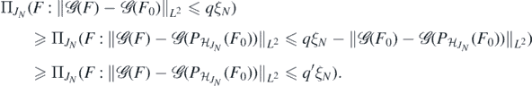
Proof of theorem 5. The conclusions of theorem 4 can readily be translated for the push-forward posterior  from (15). In particular, (13) implies, for f0 = Φ◦F0, as N → ∞,

and using lemma 29 in Nickl et al (2020) and (14) we obtain for sufficiently large M' > 0
From the previous bounds we now obtain the following result.□
Lemma 11. For ΠN(⋅|Y(N), X(N)), δN and F0 as in theorem 4, let  be the push-forward posterior distribution from (15). Then, for f0 = Φ◦F0 and any D > 0 there exists L > 0 large enough such that, as N → ∞,

Proof. Using the continuous imbedding of  , and (27), for some M' > 0 as N → ∞,

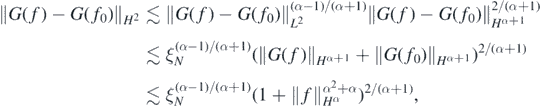
Now if f ∈ Hβ with  , lemma 23 in Nickl et al (2020) implies G(f), G(f0) ∈ Hβ+1, with

and by the usual interpolation inequality for Sobolev spaces (Lions and Magenes 1972),
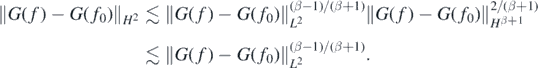
Thus, by what precedes and (26), for sufficiently large L > 0
as N → ∞.□
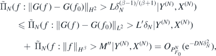
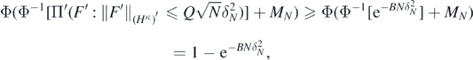
To prove theorem 5 we use (25), (27) and lemma 11 to the effect that for any D > 0 we can find L, M > 0 large enough such that, as N → ∞,
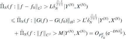
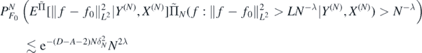
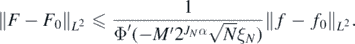
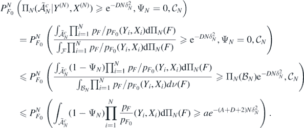
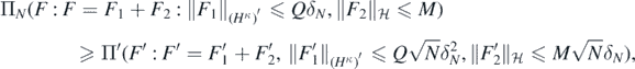
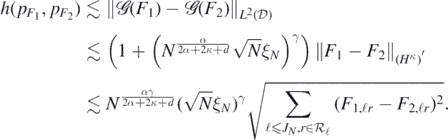
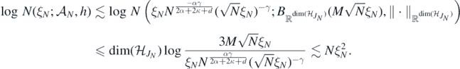
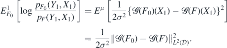
Proof of theorem 6. The proof largely follows ideas of Monard et al (2020) but requires a slightly more involved, iterative uniform integrability argument to also control the probability of events  on whose complements we can subsequently exploit regularity properties of the inverse link function Φ−1.
Using Jensen's inequality, it is enough to show, as N → ∞,

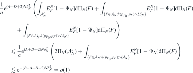
For M > 0 sufficiently large to be chosen, we decompose

Using the Cauchy–Schwarz inequality we can upper bound the expectation in the second summand by

In view of (14), for all D > 0 we can choose M > 0 large enough to obtain
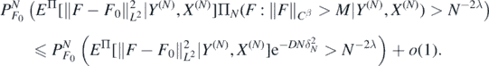
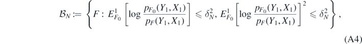
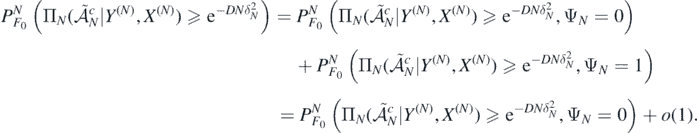
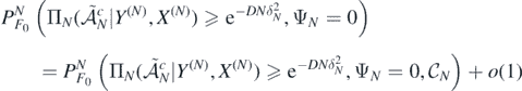
To bound the probability in the last line, let  be the sets defined in (A4) below, note that lemmas 16 and 23 below jointly imply that
  for some a,A > 0. Also, let
  , and let
  be the event from (A10), for which lemma 7.3.2 in Giné and Nickl (2016) implies that
  as N → ∞. Then
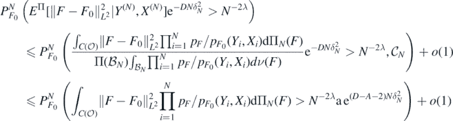
which is upper bounded, using Markov's inequality and Fubini's theorem, by
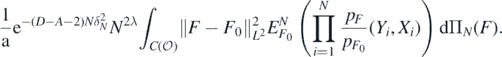
Taking D > A + 2 (and M large enough in (28)), using the fact that  , and that
  (by Fernique's theorem, e.g., Giné and Nickl (2016), exercise 2.1.5), we then conclude

To handle the first term in (28), let f = Φ◦F and f0 = Φ◦F0. Then for all  , by the mean value and inverse function theorems,

for some η lying between f(x) and f0(x). If  then, as Φ is strictly increasing, necessarily f(x) = Φ(F(x)) ∈ [Φ(−M), Φ(M)] for all
  . Similarly, the range of f0 is contained in the compact interval [Φ(−M), Φ(M)] for M ⩾ ||F0||∞, so that

for a multiplicative constant not depending on  . It follows

and

Noting that for each L > 0 the last expectation is upper bounded by
we can repeat the above argument, with the event  replaced by the event
  , to deduce from theorem 5 that for D > A + 2 there exists L > 0 large enough such that
which combined with (29) and the definition of δN concludes the proof.□
3.2. Sieve prior proofs
The proof only requires minor modification from the proofs of section 2.2.1. We only discuss here the main points: one first applies the L2-prediction risk theorem 14 with a sieve prior. In the proof of the small ball lemma 16 one uses the following observations: the projection  of
of  defined in (B4) satisfies by (B6)

hence choosing J such that 2J ≃ N1/(2α+2+d), and noting also that  for all J by standard properties of wavelet bases, it follows from (23) that

Therefore, by the triangle inequality,

The rest of the proof of lemma 16 then carries over (with  replacing F0), upon noting that (B3) and a Sobolev imbedding imply

for some constant c > 0 independent of J. Moreover, the last two properties are sufficient to prove an analogue of lemma 17 as well, so that theorem 14 indeed applies to the sieve prior. The proof from here onwards is identical to the ones of theorems 4–6 for the unsieved case, using also that what precedes implies that  , relevant in the proof of convergence of the posterior mean.
3.3. Proofs for section 2.2.3
Inspection of the proofs for rescaled priors implies that theorems 9 and 10 can be deduced from theorem 8 if we can show that posterior draws lie in a α-Sobolev ball of fixed radius with sufficiently high frequentist probability. This is the content of the next result.
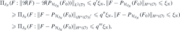
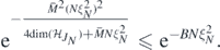
Lemma 12. Under the hypotheses of theorem 9, there exists α* > 0 (depending on α, d and a) such that for each  , and any D > 0 we can find M > 0 large enough such that, as N → ∞,

Proof. Theorem 8 implies that for all D > 0 and sufficiently large L, M > 0, if  and denoting by

then as N → ∞

Next, note that if  , then by standard properties of wavelet bases (cf. (63)),
  for all N large enough. Thus, for
  the projection of F0 onto
  defined in (B4),

and a Sobolev imbedding further gives  , for some M' > 0. Now letting f = Φ◦F and f0 = Φ◦F0, by similar argument as in the proof of theorem 6 combined with monotonicity of Φ', we see that for all N large enough
Then, using the assumption on the left tail of Φ in condition 2, and the stability estimate (25),

Finally, by the interpolation inequality for Sobolev spaces (Lions and Magenes1972) and lemma 23 in Nickl et al (2020),
so that, in conclusion, for each  and sufficiently large N,

The last term is bounded, using lemma 29 in Nickl et al (2020), by a multiple of

the last identity holding up to a log factor. Hence, if

then we conclude overall that  as N → ∞ for all
  , proving the claim in view of (30).□
Replacing β by α in the conclusion of lemma 11, the proof of theorem 9 now proceeds as in the proof of theorem 5 without further modification. Likewise, theorem 10 can be shown following the same argument as in the proof of theorem 6, noting that for Π the random series prior in (19), it also holds that  .
.
Acknowledgments
The authors are grateful to three anonymous referees for critical remarks and suggestions, as well as to Sven Wang for helpful discussions. We further acknowledge support by the European Research Council under ERC Grant agreement No. 647812 (UQMSI).
Appendix A.: Results for general inverse problems
Let  , be a nonempty open and bounded set with smooth boundary, and assume that
  is a nonempty and bounded measurable subset of
  . Let
. Let  be endowed with the trace Borel σ-field of
  , and consider a Borel-measurable 'forward mapping'

For  , we are given noisy discrete measurements of
  over a grid of points drawn uniformly at random on
  ,
,

for some σ > 0. Above μ denotes the uniform (probability) distribution on  and the design variables
  are independent of the noise vector
  . We assume without loss of generality that
  , so that μ = dx, the Lebesgue measure on
  .
.
We take the noise amplitude σ > 0 in (A1) to be fixed and known, and work under the assumption that the forward map  satisfies the following local Lipschitz condition: for given β, γ, κ ⩾ 0, and all
  ,
,

where we recall that X* denotes the topological dual Banach space of a normed linear space X. Additionally, we will require  to be uniformly bounded on its domain:

As observed in (23), the elliptic inverse problem considered in this paper falls in this general framework, which also encompasses other examples of nonlinear inverse problems such as those involving the Schrödinger equation considered in Nickl et al (2020) and Nickl (2018), for which the results in this section would apply as well. It also includes many linear inverse problems such as the classical Radon transform, see Nickl et al (2020).
A.1. General contraction rates in Hellinger distance
Using the same notation as in section 2.1.2, and given a sequence of Borel prior probability measures ΠN on  , we write ΠN(⋅|Y(N), X(N)) for the posterior distribution of F|(Y(N), X(N)) (arising as after (9) and (10)). We also continue to use the notation pF for the densities from (8) now in the general observation model (A1) (and implicitly assume that the map (F, (y, x)) ↦ pF(y, x) is jointly measurable to ensure existence of the posterior distribution). Below we formulate a general contraction theorem in the Hellinger distance that forms the basis of the proofs of the main results. It closely follows the general theory in Ghosal and van der Vaart (2017) and its adaptation to the inverse problem setting in Monard et al (2020)—we include a proof for conciseness and convenience of the reader.
Define the Hellinger distance h(⋅, ⋅) on the set of probabilities density functions on  (with respect to the product measure dy × dx) by
For any set  of such densities, let
  , be the minimal number of Hellinger balls of radius η needed to cover
  .
.
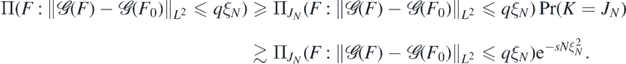
Theorem 13. Let ΠN be a sequence of prior Borel probability measures on  , and let ΠN(⋅|Y(N), X(N)) be the resulting posterior distribution arising from observations (Y(N), X(N)) in model (A1). Assume that for some fixed
  , and a sequence δN > 0 such that δN → 0 and
  as N → ∞, the sets
satisfy for all N large enough

Further assume that there exists a sequence of Borel sets  for which

for all N large enough, as well as

Then, for sufficiently large L = L(B, C) > 4 such that L2 > 12(B ∨ C), and all 0 < D < B − A − 2, as N → ∞,

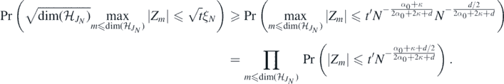
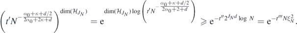
Proof. We start noting that by theorem 7.1.4 in Giné and Nickl (2016), for each L > 4 satisfying L2 > 12(B ∨ C) we can find tests (random indicator functions) ΨN = ΨN(Y(N), X(N)) such that as N → ∞

Next, denote the set whose posterior probability we want to lower bound by

and, using the first display in (A9), decompose the probability of interest as
Next, let  be the restricted normalised prior on
  , and define the event

for which lemma 7.3.2 in Giné and Nickl (2016) implies that  as N → ∞. We then further decompose
and in view of condition (A5) and the above definition of  , we see that
We conclude applying Markov's inequality and Fubini's theorem, jointly with the fact that for all 

to upper bound the last probability by
as N → ∞ since B > A + D + 2, having used the excess mass condition (A6) and the second display in (A9).□
A.2. Contraction rates for rescaled Gaussian priors
While the previous result assumed a general sequence of priors, we now derive explicit contraction rates in L2-prediction risk for the specific choices of priors considered in section 2.2. We start with the 're-scaled' priors of section 2.2.1.
Theorem 14. Let the forward map  satisfy (A2) and (A3) for given β, γ, κ ⩾ 0 and S > 0. For integer α > β + d/2, consider a Gaussian prior ΠN constructed as in (11) with scaling Nd/(4α+4κ+2d) and with base prior F' ∼ Π' satisfying condition 3 with RKHS
  . Let ΠN(⋅|Y(N), X(N)) be the resulting posterior arising from observations (Y(N), X(N)) in (A1), assume
  and set δN = N−(α+κ)/(2α+2κ+d).
Then for any D > 0 there exists L > 0 large enough (depending on σ, F0, D, α, and β, γ, κ, S, d) such that, as N → ∞,

and for sufficiently large M > 0 (depending on σ, D, α, β, γ, κ, d)

Remark 15. Inspection of the proof shows that if κ=0 in (A12), then the RKHS  in condition 3 can be assumed to be continuously imbedded in Hα(
 ) only instead of Hαc(
 ). The same remark in fact applies for κ < 1/2.
Proof. In view of the boundedness assumption (A3) on  , we have by lemma 23 below that for some q > 0 (depending on σ, S)

Hence, for  the sets from (A4) we have
  which in turn implies the small ball condition (A5) since by lemma 16 below (premultiplying if needed δN by a sufficiently large but fixed constant):

for some A > 0 and all N large enough. Next, for all D > 0 and any B > A + D + 2, we can choose sets  as in lemmas 17 and 18 and verify the excess mass condition (A6) as well as the complexity bound (A7). Note that
  for all
  . We then conclude by theorem 13 that for some L' > 0 large enough

yielding the claim for some appropriate L > 0 using the first inequality in (A26).□
The following key lemma shows that the (non-Gaussian) prior induced on the regression functions  assigns sufficient mass to a L2-neighbourhood of
  .
.
Lemma 16. Let ΠN, F0 and δN be as in theorem 14. Then, for all sufficiently large q > 0 there exists A > 0 (depending on q, F0, α, β, γ, κ, d) such that

for all N large enough.
Proof. Using (A2) and noting that  for
for  by a Sobolev imbedding, for any fixed constant M > 1∨ ||F0||Cβ,

having defined

whose intersection is a symmetric set in the ambient space  . Then, since
  , recalling that the RKHS
  of ΠN coincides with
  with RKHS norm
  given in (12), now with scaling
  , we can use corollary 2.6.18 in Giné and Nickl (2016) to lower bound the last probability by
We proceed finding a lower bound for the prior probability of C1, which, by construction of ΠN, satisfies

For any integer α > 0 and any κ ⩾ 0, letting  , we have the metric entropy estimate:

see the proof of lemma 19 in Nickl et al (2020) for the case κ ⩾ 1/2, and theorem 4.10.3 in Triebel (1978) for κ < 1/2 (in the latter case, we note in fact that the estimate holds true also for balls in the whole space Hα). Hence, since  is continuously imbedded into
  , letting
  be the unit ball of
  , we have
  for some r > 0, implying that for all η > 0

Then, for all N large enough, the small ball estimate in theorem 1.2 in Li and Linde (1999) yields
implying  for some q'' > 0. Note that q'' can be made as small as desired by taking q in (A13) large enough.
We conclude obtaining a suitable upper bound for ΠN(C2c). In particular, by construction of ΠN, recalling  ,
,

By condition 3, F' defines a centred Gaussian Borel random element in a separable measurable subspace  of Cβ, and by the Hahn–Banach theorem and the separability of
  ,
,  can then be represented as a countable supremum

of actions of bounded linear functionals  . It follows that the collection
  is a centred Gaussian process with almost surely finite supremum, so that by Fernique's theorem Giné and Nickl (2016), theorem 2.1.20:

We then apply the Borell–Sudakov–Tirelson inequality Giné and Nickl (2016), theorem 2.5.8, to obtain for all N large enough,

Given our initial choice of M, the proof is then concluded taking q in lemma 16 sufficiently large so that q'' < (M/τ)2/8.□
We now construct suitable approximating sets for which we check the excess mass condition (A6).
Lemma 17. Let ΠN and δN be as in theorem 14. Define for any M, Q > 0

Then for any B > 0 and for sufficiently large M, Q (both depending on B, α, β, γ, κ, d), for all N large enough,

Proof. We note that the last inequality at the end of the proof of the previous lemma implies that for  and all N large enough,
  Thus, the claim will follow if we can derive a similar lower bound for
having used that  . Using theorem 1.2 in Li and Linde (1999) as before (A15), we deduce that for some q > 0

so that taking any Q > (B/q)−(2α+2κ−d)/(2d) implies

Next, denote
where Φ is the standard normal cumulative distribution function. Then by standard inequalities for Φ−1 we have  as N → ∞, so that taking
By the isoperimetric inequality for Gaussian processes Giné and Nickl (2016), theorem 2.6.12, the last probability is then lower bounded, using (A18), by
concluding the proof.□
We conclude with the verification of the complexity bound (A7) for the sets  .
.
Lemma 18. Let  be as in lemma 17 for some fixed M, Q > 0. Then,
for some constant C > 0 (depending on σ, M, Q, α, β, γ, κ, d, S) and all N large enough.
Proof. If  , then F = F1 + F2 with
  and
and  the latter inequality following from the continuous imbedding of
  into
into  . Thus, recalling the metric entropy estimate (A14), if

is a δN-net with respect to  , we can find Hi such that
  . Then, using the second inequality in (A26) below and the local Lipschitz estimate (A2),

Recalling that if  then also
  , and using the Sobolev imbedding of Hα into Cβ to bound
  , we then obtain

It follows that {H1, ..., HP} also forms a q'δN-net for  in the Hellinger distance for some q' > 0, so that

□
A.3. Contraction rates for hierarchical Gaussian series priors
We now derive contraction rates in L2-prediction risk in the inverse problem (A1), for the truncated Gaussian random series priors introduced in section 2.2.3. The proof again proceeds by an application of theorem 13.
Theorem 19. Let the forward map  satisfy (A2) and (A3) for given β, γ, κ ⩾ 0 and S > 0. For any α > β + d/2, let Π be the random series prior in (19), and let Π(⋅|Y(N), X(N)) be the resulting posterior distribution arising from observations (Y(N), X(N)) in (A1). Then, for each α0 ⩾ α, any
  and any D > 0 there exists L > 0 large enough (depending on σ, F0, D, α, β, γ, κ, S, d) such that, as N → ∞,

where  . Moreover, for
  the finite-dimensional subspaces from (18) and
  such that
  , we also have that for sufficiently large M > 0 (depending on D, α, β, d):

We begin deriving a suitable small ball estimate in the L2-prediction risk.
Lemma 20. Let Π, F0 and ξN be as in theorem 19. Then, for all sufficiently large q > 0 there exists A > 0 (depending on q, F0, α, β, γ, κ, d) such that

for all N large enough.
Proof. For each  , denote by Πj the Gaussian probability measure on the finite dimensional subspace
  in (18) defined as after (19) with the series truncated at j. For
  , note

so that, recalling the properties (20) of the random truncation level J, for some s > 0,

for all N large enough. It follows
Next, let
be the 'projection' of F0 onto  . Since
  by a Sobolev imbedding, it follows using (A2) and standard approximation properties of wavelets (B6),

which implies by the triangle inequality that
Using again that Hα imbeds continuously into Cβ as well as (A2) and (B5), we can lower bound the last probability by
which, by corollary 2.6.18 in Giné and Nickl (2016) and in view of (B2) is further lower bounded by

Now since  , is continuous on
  ,
,
for some t > 0, where  , and where we have used the wavelet characterisation of the
  norm. To conclude, note that the last probability is greater than
Finally, a standard calculation shows that Pr(|Z1| ⩽ t) ≳ t if t → 0, and hence the last product is lower bounded, for large N, by
□
In the following lemma we construct suitable approximating sets, for which we check the excess mass condition (A6) and the complexity bound (A7) required in theorem 13.
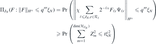
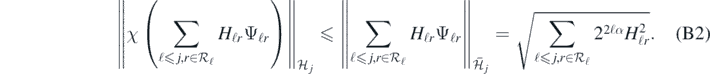
Lemma 21. Let Π, ξN and JN be as in theorem 8, and let  be the finite dimensional subspace defined in (18) with J = JN. Define for each M > 0

Then, for any B > 0 there exists M > 0 large enough (depending on B, α, β, d) such that, for sufficiently large N

Moreover, for each fixed M > 0 and all N large enough

for some C > 0 (depending on σ, α, β, γ, κ, S, d).
Proof. Letting  , noting
  for all
  (cf. (B2)) and using (A22) and (20), we have for sufficiently large N
for any constant  , since
  . The bound (A24) then follows applying theorem 3.1.9 in Giné and Nickl (2016) to upper bound the last probability, for any B > and for sufficiently large M and
  , by
, by
We proceed with the derivation of (A25). By choice of JN, if  then
then  Hence, by the second inequality in (A26), using (A2) and the Sobolev imbedding of Hα into Cβ, if
  then
then
Therefore, using the standard metric entropy estimate for balls  , in Euclidean spaces (Giné and Nickl (2016), proposition 4.3.34), we see that for N large enough
□
A.4. Information theoretic inequalities
In the following lemma due to Birgé (2004) we exploit the boundedness assumption (A3) on  to show the equivalence between the Hellinger distance appearing in the conclusion of theorem 13 and the L2-distance on the 'regression functions'
  .
.
Lemma 22. Let the forward map  satisfy (A3) for some S > 0. Then, for all
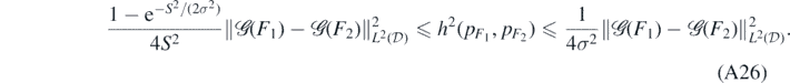

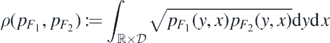
is the Hellinger affinity. Using the expression of the likelihood in (8) (with  instead of
  ), the right hand side is seen to be equal to
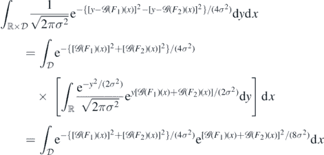
having used that the moment generating function of Z ∼ N(0, σ2) satisfies  . Thus, the latter integral equals

To derive the second inequality in (A26), we use Jensen's inequality to lower bound the expectation in the last line by

Hence
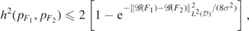
whereby the claim follows using the basic inequality 1 − e−z/c ⩽ z/c, for all c, z > 0.
To deduce the first inequality we follow the proof of proposition 1 in Birgé (2004): note that for all 0 ⩽ z1 < z2
Then taking  and z2 = S2/(2σ2),

which in turn yields the result.□
The next lemma bounds the Kullback–Leibler divergences appearing in (A4) in terms of the L2-prediction risk.
Lemma 23. Let the observation Yi in (A1) be generated by some fixed  . Then, for each
  ,
,
and

Hence, since EW1 = 0 and X1 ∼ μ,
On the other hand,
whence the second claim follows since  .□
.□
Appendix B.: Additional background material
In this final appendix we collect some standard materials used in the proofs for convenience of the reader.

and let  be a smooth compactly supported function such that
  . Define for any Kmin ∈ (0, 1)

Then it is elementary to check that Φ is a regular link function that satisfies condition 2 (with a = 2).
Example 25. For any real α > d/2, the Whittle–Matérn process with index set  and regularity α − d/2 > 0 (cf. example 11.8 in Ghosal and van der Vaart (2017) is the stationary centred Gaussian process
  with covariance kernel

From the results in chapter 11 in (Ghosal and van der Vaart 2017) we see that the RKHS of  equals the set of restrictions to
  of elements in the Sobolev space
  , which equals, with equivalent norms, the space
  (since
  has a smooth boundary). Moreover, lemma I.4 in Ghosal and van der Vaart (2017) shows that M has a version with paths belonging almost surely to Cβ' for all β' < α − d/2. Let now
  be a nonempty compact set, and let M be a Cβ'-smooth version of a Whittle–Matérn process on
  with RKHS
  . Taking F' = χM implies (cf. exercise 2.6.5 in Giné and Nickl (2016)) that
  defines a centred Gaussian probability measure supported on Cβ', whose RKHS is given by
and the RKHS norm satisfies that for all  there exists
  such that χF = χF* and

Thus if F' = χF is an arbitrary element of  , then

which shows that  is continuously embedded into
  .
.
Remark 26. Let  be an orthonormal basis of
  composed of S-regular and compactly supported Daubechies wavelets (see chapter 4 in Giné and Nickl (2016) for construction and properties). For each 0 ⩽ α ⩽ S, we have
and the square root of the latter series defines an equivalent norm to  . Note that S > 0 can be taken arbitrarily large.
For any α ⩾ 0 the Gaussian random series
defines a centred Gaussian probability measure supported on the finite-dimensional space  spanned by the
  , and its RKHS equals
  endowed with norm
(cf. example 2.6.15 in Giné and Nickl 2016). Basic wavelet theory implies  .
.
If we now fix compact  such that K ⊊ K', and consider a cut-off function
  such that χ = 1 on K', then multiplication by χ is a bounded linear operator
  It follows that the random function
defines, according to exercise 2.6.5 in Giné and Nickl (2016), a centred Gaussian probability measure  supported on the finite dimensional subspace
  from (18), with RKHS norm satisfying
Arguing as in the previous remark one shows further that for some constant c > 0,

Remark 27. Using the notation of the previous remark, for fixed  , consider the finite-dimensional approximations

Then in view of (B2), we readily check that for each j ⩾ 1

Also, for each κ ⩾ 0, and any  , we see that (implicitly extending to 0 on
  functions that are compactly supported inside
  )
)

where  , with χ' = 1 on supp(χ). We also note that, in view of the localisation properties of Daubechies wavelets, for some
  large enough, if ℓ ⩾ Jmin and the support of Ψℓr intersects K, then necessarily supp(Ψℓr) ⊆ K', so that

Therefore, for j ⩾ Jmin, by Parseval's identity and the Cauchy–Schwarz inequality
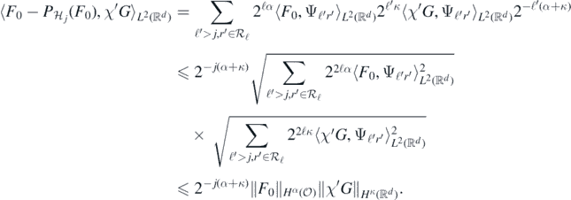
It follows by duality that for all j large enough

We conclude remarking that

Indeed, let j ⩾ Jmin, and fix  ; then

But as  is a fixed finite dimensional subspace, then we have
  for some fixed multiplicative constant only depending on Jmin. On the other hand, we also have
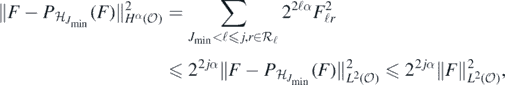
yielding (B7).
Example 28. Consider the integer-valued random variable

where ϕ(x) = x log x, x ⩾ 1. Then for any j ⩾ 1

On the other hand, since  as j → ∞,