
Abstract
Azimuth and distance measurement are two key technologies of MEMS LIDAR. In order to improve the accuracy of (micro-electronical mechanical system scanning mirror) MEMS-SM angle measurement, this paper proposes an angle estimation algorithm based on unscented Kalman filter (UKF), which can reduce the sensor noise by using the motion model of MEMS-SM. First, the angle measurement is given by the built-in angle sensor or transfer function model of MEMS-SM. Secondly, the dynamic model is established according to the Lissajous scanning mode of MEMS-SM. Then the UKF algorithm can be presented, including the measurement equation and the state equation, where the nonlinear equation is the inverse trigonometric function. Finally, Laser Doppler Velocimeter was adopted as a standard instrument to verify the accuracy of the proposed algorithm. The results showed that the UKF angle estimation algorithm based on MEMS-SM dynamic model improved the accuracy of the built-in sensor's angle measurement by 5–10 times. And this method is suitable for LIDAR of different scanners' types and different scanning modes, which can meet the demand of imaging MEMS LIDAR for the accuracy and stability of angle measurement.
Export citation and abstract BibTeX RIS

Original content from this work may be used under the terms of the Creative Commons Attribution 3.0 licence. Any further distribution of this work must maintain attribution to the author(s) and the title of the work, journal citation and DOI.
1. Introduction
Micro-electronical mechanical system scanning mirror (MEMS-SM) has gained vastly in interest over the last decades, and is, by now, deployed in various fields. Its application ranges from laser pico-projectors [1, 2], laser tracking on UAV (unmanned aerial vehicle) [3], dynamic solid state lighting [4], to MEMS imaging LiDAR (light detection and ranging) [5, 6]. The application on MEMS imaging LiDAR grows especially fast in the last 5 years, with the rise of autopilot technology. The angle measurement technique of the MEMS-SM has undergone a history from theory analysis, external calibration to internal calibration. Among them, the theory analysis (based on dynamic characteristics of electrostatically driven MEMS-SM [7, 8]) can only obtain a theoretical relationship between the input voltage and the output angle. Compared to the theory analysis method, the external calibration methods, which include laser interferometric method [9], triangulation [10, 11], 2D PSD (position sensitive detector) [12, 13] and light barrier [14] have very high angle measurement accuracy, but the measuring system is very complex and is not suitable for on-line measurement. So some people have carried out research in a way of internal angle calibration. This research is based on built-in sensors, such as capacitance sensor [15], piezo-resistive sensor [16] and etc. The advantage of internal angle calibration is that the angle can be measured in real-time, however, these silicon-based sensors are easy to be influenced by temperature, and the sensors themselves also have zero drifting. The highest precision that can be reached by this method is 0.04° [17]. In 2017, Faller and Hubert [18] in Alpen-Adria-Universität Klagenfurt used EKF (extended Kalman filter) to estimate the angle of the MEMS-SM which is a part of a Michelson interferometer setup, and the angle sensor is made of inkjet-printed capacitive position sensor, they can get the high required position resolution of respos < 50 nm in the range of rm = 1000 µm.
On the one hand, MEMS-SM has three modes of scanning [3], the Linescan and Lissajous modes are widely used [19, 20]. These two types of scanning modes are standard dynamic vibration, the drive signals are sinusoidal wave and triangular wave. So the kinetic equation can be built up, which is used for state equations. On the other hand, the measured by angle sensor is used as measurement equations. Since the dynamic equation of MEMS-SM is a sine function, the inverse trigonometric transformation can be used for measurement equation in UKF (unscented Kalman filter). The MEMS-SM device used in this paper comes from the literature [17].
2. MEMS LIDAR and MEMS-SM
2.1. MEMS LIDAR
LiDAR is a radar with laser as carrier wave. It can obtain the target's characteristic parameters such as distance, azimuth, reflectivity, speed and other information by demodulating the target modulation information carried by the wave signal. The initial application was mainly in the military field, providing high-resolution radiation intensity geometric images, distance images, and speed images, and thus received great attention from the military departments of various countries. The working principle of the 3D imaging laser radar is to realize the scanning measurement imaging of the target 3D contour through laser ranging and scanning angle measurement. With the development of the automatic driving technology (figure 1), the 3D imaging laser radar has received extensive attention as the most important environment-sensing sensor. Compared to motor-driven mechanical laser radars, solid-state LIDAR based on MEMS-SM, OPA (optical phased arrays), 3D FLASH, and DMD (digital micromirror device) have huge advantages in terms of volume, power consumption, and cost, as key device MEMS-SM goes matures. MEMS-based MEMS LIDAR has become a research hotspot.
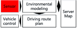
Figure 1. Autopilot technical principles.
Download figure:
Standard image High-resolution imageSince the concept of MEMS-based next-generation laser radar was first proposed by NIST [21] (National Institute of Standards and Technology) in 2004, LightTime Inc., the European MiniFaros Project, Technical University of Denmark (DTU), Army Research Laboratory (ARL), Yeungnam University, and other units have long-term commitment to the application of MEMS-SM to low-cost 3D imaging LIDAR. The MiniFaros project focuses on the problem of MEMS-SM angle measurement. Institutions that study MEMS-SM, such as the Adriatic Research Institute, Beckman Laser Institute, etc have also long studied their transfer function (TF) models and angle sensors.
2.2. Angle measurement sensor in the MEMS LIDAR
Piezoresistive sensors are widely used in the measurement of physical quantities such as stress and acceleration, and they are compatible with MEMS-based silicon technology. They are inexpensive and easy to batch. With the back-end bridge measurement circuit, high-precision angle measurement can be achieved. MEMS-SM built-in angle sensor technology research. The previous research results [16] of the research group and the later improvements [17] have achieved a theoretically high-precision angle measurement of 0.044°. The schematics of the scan mirror layout and angle measurement principle are shown below.
It can be seen from the position (figures 2(a) and (b)), and the crystal orientation (figure 2(c)) of the piezoresistive material. Among them,  are piezoresistive sensors longitudinal, lateral and tangential piezoresistive coefficient respectively. The relationship between normal stress
  and shear stress
  and rotation angle is as follows:
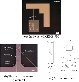
Figure 2. Previous research results.
Download figure:
Standard image High-resolution imageAmong them,  is the Young's modulus,
  is the shear modulus,
  is the positive and shear stress torsional coefficient of the rectangular section bar,
  are the thickness and length of the beam.
Through a single-arm bridge, the resistance change of the piezoresistive sensor is converted into a voltage change output [22]

Bringing equation (1) into (2) yields the relationship between the output voltage and the micro-mirror vibration angle:
3. UKF algorithm
Kalman filtering is a well-known estimation technique, used to recover signals from noisy measurements. Its applications range from integrated navigation [23, 24], pose estimation [25, 26], to control of torsional micro-mirrors [27]. It is suitable for solving problems where motion tracking of dynamic systems, which are either nonlinear in their dynamics [28] or in the real-time measurement, is desired at the least computation. The standard KF algorithm can only deal with the linear system, so it was proposed to linearize the nonlinear system using the Taylor series expansion method. Because it only took the first two items of Taylor expansion, there is not high accuracy and fast change speed. The goal reflects delays and other issues. In order to solve the problems of EKF, Julier and Ohlmann proposed the UKF [29].
Consider the following nonlinear system, described by the difference equation and the observation model with additive noise:
where  represent the unobserved state of the system,
  is the observed measurement signal. The process noise
  drives the dynamic system, and the observation noise is given by
  . Note that we are not assuming additivity of the noise sources. The system dynamic model f and h are assumed known.
3.1. Lissajous-scanning and process model
Tracking of triangular or sawtooth waveforms is a major difficulty for achieving high-speed operation in many scanning applications such as atomic force microscopy [30], MEMS-SM [31]. Such non-smooth waveforms contain high order harmonics of the scan frequency that can excite mechanical resonant modes of the positioning system, limiting the scan range and bandwidth. The Lissajous-scan pattern can be generated by forcing the bending and twisting axes of the scanner to track the following signals:
Because the bending-axes and the twisting-axes are both single frequency sinusoidal signal, the Lissagous-scanning method will not interfere with the system.
Since the two-axis vibration of MEMS-SM is orthogonal and the resonant frequency is different, the output voltage  in equation (3) contains two frequency components
  and
and  . After passing through two band-pass filters, the two frequencies are separated. Have:
So far, in the Lissagous-scanning mode, we can get the vibration angle of the two axes of 2D MEMS-SM from  and
and  . We supposed:
And set the  , we can get the following formula:
However, the f is the sinusoidal function.
3.2. Measurement model
Different MEMS-SM has different measurement methods, so we try to establish a unified measurement model. This article uses three types of MEMS micromirrors, namely electromagnetic, electrostatic and piezoelectric. And there are two ways to measure the angle, as mentioned above, they are piezo-resistive sensor and TF [8].
From the [8], we can get the TF of the MEMS-SM is the second order system, the general expression is:
And the parameter are all in the same reference.
The measuring equation h will be the TF if we use the electromagnetic MEMS-SM. And as well, it also will be the angle sensor output (for example, the equation (3)) if we use the MEMS-SM which has the angle sensor like piezo-resistive sensor.
3.3. Design UKF
The UKF is a suboptimal estimator based on linear minimum mean square error (LMMSE) estimation and analytic linearisation [32]. Unlike the EKF, the UKF algorithm takes the nonlinear transformation UT transformation as the core and does not need to linearize the state equation and the observation equation. It directly uses the nonlinear state equation to estimate the probability density function (PDF) of the state vector, through the deterministic sampling strategy. A set of Sigma points was selected from the original state distribution to make the sample mean and covariance consistent with the mean and covariance of the state variables. Then, nonlinear transformations are performed on these points to obtain the mean and covariance of the transformation points. When the PDF of the state vector is Gaussian, the mean and covariance of the Gaussian density function can be obtained by using this set of sampling points. When a Gaussian state vector is transmitted via a non-linear system, for any kind of nonlinear system, this set of sampling points can be used to obtain the posterior mean and covariance of the third moment.
According to the two resonance vibration modes of MEMS-SM [16]. The vibration of the mirror has states corresponding to time, driving voltage and the angle.

The two axes of the Lissajous figure are standard sine waves, so the micromirror rotation angle also changes in the form of a sine wave of this frequency. Assuming that the initial angle  , The micro-mirror oscillation frequency is
  and the sampling period is
  . There are the following relations:


Let ![$s(k)=\arcsin \left[ \frac{x(k)}{A} \right]$](https://content.cld.iop.org/journals/0960-1317/29/3/035005/revision2/jmmaaf943ieqn021.gif) , then here is a state equation:
, then here is a state equation:

The rotation angle of the micromirror is proportional to the voltage, and the observation equation is:

Bring  into the above equation, the observable equation is:

In the simulation, there is no error due to the initial value, that is,  and
and  are all set to 0. The driving voltage is a sinusoidal signal, and its stability is the process noise covariance
  . When the driving voltage is 0, the variance of the angle sensor output value is R.
4. LDV-based calibration method
4.1. LDV angle measurement principle and accuracy analysis
A method of laser micro-angle calibration based on LDV was designed. As shown in the figure below, in the case of uniaxial scanning, assuming that point O is the fixed point of the MEMS-SM, the spot of the LDV irradiates at point A when there is no angle swing, and when the MEMS-SM swings at a certain angle Ф, the spot shines on point B, the real-time distance between AB can be measured by LDV.
According to the schematic principle (figure 3), the real-time rotation angle Ф of MEMS-SM can be obtained:
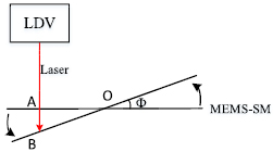
Figure 3. Laser Doppler vibrometer (LDV) angle measurement principle.
Download figure:
Standard image High-resolution imageIn this paper, the OFV-534 laser probe manufactured by Polytech Co., Ltd was used to measure with the OFV-5000 LDV controller. Instrument manual ranging uncertainty is  . The image sensor in the microscope is 510 * 492 pixels, and the field of view is 3.8 mm * 2.9 mm. Take the single pixel width as its uncertainty:
According to the actual situation, as shown in the following figure, the fixed point of the piezoelectric MEMS-SM is O, and the appropriate measurement point A is selected so that its coordinates are (0, 900 µm). When the MEMS-SM vibrates uniaxially along the x-axis, If the MEMS-SM rotation amplitude is 0.05°, according to equation (17) we can see that AB ≈ 0.79 µm.
The uncertainty formula is as follows:
When the swing angle is 0.05°,  is approximately 0.009 64°, and therefore it is possible to correct the output angle of the angle measuring sensor using the measured value of LDV as a true value.
As can be seen from the figure 4, first, the UKF-based angle estimate is approximately two orders of magnitude lower than the direct sensor angle measurement error; second, the UKF-based angle estimation error exhibits periodicity, indicating that there is a delay between truth value and UKF estimate value.
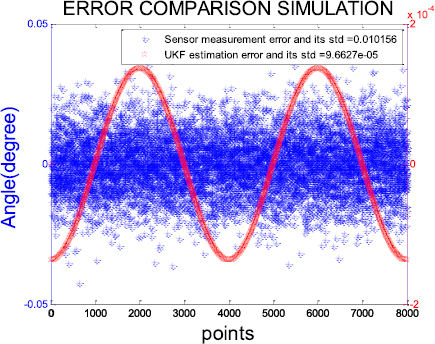
Figure 4. Error comparison between the UKF estimate and the sensor's direct output angle.
Download figure:
Standard image High-resolution image4.2. Experimental preparation
Due to the limitation of the measuring range of the LDV, the limiting micromirror is uniaxially oscillating, and the amplitude of the oscillation is −5° to +5° (i.e. (−0.087 to +0.087 rad)).
The experiment uses four-channel oscilloscope to collect LDV, sensor angle data and drive signal at the same time to ensure the time synchronization of the data. The off-line method uses the drive signal to establish the dynamic equation of UKF, and uses the sensor data to establish the measurement equation of UKF. After the analysis in section 4.1, we can see that the LDV data can be used as the true value of the angle.
Using two commercial MEMS-SMs for comparison. One is the CW1012-MEMS-SM from Changzhou Micro Innovation Inc. has an angle sensor in it. This MEMS-SM operates on its fast axis at its resonant frequency of 14 510 Hz and its slow axis operates around 200 Hz. This micro-mirror is electromagnetic type, with a built-in angle sensor, the rotation angle accuracy is 2 µrad, the angle sensor sensitivity is 3 mV V−1@1 rad. In the experiment, the input signal of the micromirror fast axis was 0.5 V and the frequency was 14 510 Hz. In figure 5, the first channel is the LDV distance data, the second channel is the control signal data, and the third channel is the sensor angle measurement data. The other comes from Mirrorcle Inc., micro-mirror ID: S30348, drive model: A7M20.1. It belongs to the electrostatic type, and its interior is not equipped with an angle sensor, and the nominal angle repeat accuracy is 0.0005°. The TF between the control voltage and the angle is shown in the [8]. The drive signal is a standard sinusoid with a peak-to-peak value of 4 V, a drive frequency of 800 Hz, and an oscilloscope sampling frequency of 1 MHz. In figure 6, the first channel is LDV distance data, and the second channel is control signal data. The control signal data has two purposes. On the one hand, it is used to establish the dynamic equation of UKF. On the other hand, the micro-mirror's TF model can obtain the angle of the micro-mirror, and then establish the UKF's observation equation.

Figure 5. CW1012 MEMS-SM.
Download figure:
Standard image High-resolution image
Figure 6. A7M20.1 MEMS-SM.
Download figure:
Standard image High-resolution image4.3. Error analysis
The angle data from the angle sensor, LDV and UKF are shown in figure 7, and in figure 8, the calculation shows that the variance of the measurement error based on UKF is approximately 2.17 × 10⁻⁵, the variance of the measurement error of the micro-mirror's own sensor is approximately 2.17 × 10⁻⁴, and the average measurement error of the result of UKF is less than 0.05°. UKF-based angle estimation method improves the accuracy of angle measurement by nearly 8 times, and effectively suppress external noise interference.
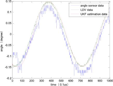
Figure 7. Angle data comparison on CW1012.
Download figure:
Standard image High-resolution image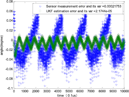
Figure 8. Angle error between UKF and angle sensor on CW1012.
Download figure:
Standard image High-resolution imageThe angle data from TF, LDV and UKF are shown in figure 9. In figure 10, the variance of the UKF angle error is about 0.0012, and the variance of the angle error using the drive voltage is about 0.0067. It can be seen that the UKF improves the measurement stability by about 6 times (the experimental data corresponds to the micro-mirror rotation range is (−1.3°, +1.3°), and the UKF error within this range of rotation is 0.05°, which meets the expected accuracy requirements). Because the use of LDV to measure the change of the micro-mirror angle, the external vibration (such as the oscilloscope button operation when the laboratory will experience a slight vibration, so that the LDV measurement when there is low-frequency interference) will also Influencing the LDV measurement results, resulting in a slight error when measuring the LDV. This data processing process does not eliminate this interference factor, but it can still be seen that UKF significantly improves the angle measurement stability and accuracy.
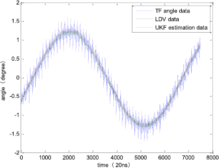
Figure 9. Angle data comparison on A7M20.1.
Download figure:
Standard image High-resolution image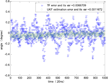
Figure 10. Angle error between UKF and TF on A7M20.1.
Download figure:
Standard image High-resolution image
The experiment verifies the feasibility of UKF in improving the MEMS-SM angle measurement accuracy. When the micromirror TF is more accurate and the accuracy of the angle sensor is 0.5°, the final average angle measurement accuracy after UKF filtering can reach 0.05°. The angle measurement is stable. Compared to the original angle measurement, angle stability is 5 to 10 times better than original angle measurement. Can support its high-precision real-time angle measurement applications in MEMS LIDAR.
5. Conclusion
First, the considered angle measured of MEMS-SM as one most important technology of a MEMS LiDAR and the suggested UKF-based angle estimation algorithm were presented. The state equation is modeled by the Lissajous motion model of the MEMS-SM, and then the measurement equation model is established based on the angular sensor measurement angle data or the angle data derived from the MEMS-SM TF, and then the UKF algorithm model is established. After mathematical analysis, the accuracy of the single-axis angle of the LDV measurement MEMS-SM can reach 0.0009°, which is taken as the true value. Comparing the angle estimation method based on the micromirror TF and the angle measurement method based on the angle sensor, the angle estimation method based on UKF proposed in this paper will improve the measurement accuracy by 5–10 times, to lay the foundation for the realization of high-precision MEMS laser radar.
Acknowledgments
This work is supported by the National Key Research and Development Program of China under the grant No. 2016YFB0500902.