

Abstract
We present an absolute energy measurement of the Kβ1,3 (KM2,3) emission spectrum of scandium (Z = 21) accurate to 2.1 parts per million (ppm). The previous experimental uncertainty was estimated as 105 ppm, or 0.47 eV, therefore we improve the accuracy of this measurement by a factor of 50 for use in any x-ray standards. There is a long-standing discrepancy between the most recent experimental and theoretical values. This work reports a Sc Kβ peak energy of 4460.845 eV with estimated standard error uncertainty of 0.0092 eV. The satellite component centroids, line-widths, and relative intensities are determined as a sum of five Voigt functions. The same analysis and experimental method shown here can be applied to advanced experiments in quantum electrodynamics, astrophysics and particle physics on soft x-ray spectra. This value has reconciled some of the previous discrepancy. However, the theoretical value is still discrepant from the new experimental measurement by 1.745 eV with a much tighter constraint on the experimental uncertainty. This strongly strengthens the need for new theoretical calculations and experimental measurements.
Export citation and abstract BibTeX RIS
1. Introduction
Spectral lines resulting from atomic transitions gave the empirical evidence needed to kick-start the quantum revolution of the early 1900s, suggesting that electronic energy states are quantised, rather than continuous. After more than a 100 years, spectral lines of electronic and exotic atoms and ions remain the primary tool to experimentally investigate theories of quantum electrodynamics (QED) [1–5] and the standard model. With new techniques, researchers have been able to probe these spectra at ever-increasing resolution and precision, showing that our current best theories still do not fully account for the observed results [6].
As well as the motivation for probing theoretical calculations of advanced quantum mechanics, there is a significant industrial motivation for tight constraints to 3d K-series energies. Lanthanides, the rare earth elements, are becoming increasingly desirable to manufacturers of electronics, lighting, and permanent magnets. Therefore there is great interest in analysing lanthanide-bearing ores by x-ray fluorescence. Since the L-series of the lanthanides is in the same energy regime as the K-series of 3d metals, tying down the uncertainties on these elements will aid in analysing materials for possible lanthanide deposits [7].
This investigation reports on the Kβ1,3 (KM2,3) transition in scandium (Z = 21) yielding a new measurement of profile and energy with standard uncertainty reduced by approximately a factor of 50. This fills a gap in the current literature. All other 3d transition metals have experimental uncertainties for the energy of Kα and Kβ less than 0.1 eV, showing that the 0.47 eV uncertainty for Sc Kβ is outdated and in need of improvement.
The Kβ1,3 transition occurs when a core (1s) electron is ejected, and a 3p electron fills the hole. The p orbital is an energy doublet of  resulting in two spectral (diagram) lines; Kβ1 from 3p3/2 → 1s and Kβ3 from 3p1/2 → 1s. However, these two spectral lines are only well-resolved in medium to high Z elements [8], unlike scandium. Along with the unresolved spectral doublet, there are satellite lines yielding asymmetries and analytical complexities in the spectral profiles.
Satellite lines exist as non-degenerate transitions to the local diagram line with smaller amplitude. Analysis of the satellites within spectra offer novel insight into complex inner-shell interactions of electrons; advanced quantum mechanics [9, 10]; spectral analysis of astrophysical phenomena [11]; chemistry [12]; and QED [3]. The leading theory explaining the origin of these satellite lines invokes the idea of shake processes [13–17], occurring when the removal of the core electron displaces another electron into the continuum (shake off), or into a higher energy orbital (shake up). The 3p → 1s transition then occurs under an altered potential resulting in a non-degenerate transition and more complex multiplet.
Relative energy measurements of the Sc Kβ1,3 profile are common [15, 18, 19]. However, there is only a single absolute energy measurement on this profile [8]. Let us clarify that absolute measurements should be calibrated in an absolute sense to the energy scale and hence to eV and to the metre [20]. A relative measurement is characterised by a reference point of the energy of some offset or scale often from a theoretical assumption [21]. This discussion is referenced to the current status on the subject [9]; suffice it to say here that we are reporting an absolute measurement and considering all significant sources of inaccuracy and not just imprecision in the measurement.
Experimental difficulties with the Sc Kβ1,3 profile arise due to its relatively low energy, explaining the lack of investigation over decades—during which all other 3d transition metals have been measured on an absolute scale. The increased sensitivity and precision for spectroscopic techniques described herein relate to any field needing calibration of soft x-rays.
Precise absolute energy measurement offers great insight for comparison with current theoretical calculations. Advanced relativistic quantum mechanical theory is improving its ability to investigate complex multiple inner-shell vacancies as required here.
2. Nomenclature and measures of central tendency
There are several reportable quantities in x-ray standards, each with distinct definitions which can lead to some confusion. Most previous authors have reported the reconstructed characterisation peak energy E , E
, E , E(Kβ0) et seq. for different characteristic profiles. These are defined as the energy of the maximum amplitude of the analytic representation of the profile with no Gaussian component. This is not the peak energy of the raw experimental data (Kα1,peak, Kα2,peak, Kβpeak et seq.) at the intrinsic experimental resolution but rather is corrected or deconvolved for (known) experimental broadening, which in principle allows it to be more portable and transferable as a standard. One advantage of this is that it removes an instrumental broadening from the profile, so is closer to a theoretical prediction, and closer to a more uniform and portable measure of central tendency. However, theoretical works may and often do report the diagram line E(Kβ1), KM3 and E(Kβ3), KM2. A discussion of the detailed theoretical (atomic) physics of the spectral profiles is out of place here, but suffice it to say that these may be the most dominant pair of (theoretical) contributors to the profile. Experimentally, advanced and recent reference standards and analysis has presented characterisations of the spectral profiles in terms of dominant components (e.g. E(Kβa), E(Kβb), E(Kβc), et seq.). The theoretical predictions may or should be close approximations to the largest two components: E(Kβa) or E(Kβb) (in our notation). Equally other measures of central tendency are often reported including the profile centre of mass (KβCoM) especially for experiments using lower resolution detectors such as Charge Coupled Device or Si(Li) or Ge detectors. Experimental (Gaussian) broadening and any asymmetries lead to these measures being unequal.
There is difficulty in comparing current x-ray standards to those set out in older works, notably the extensive tabulation given by Bearden in 1967 [8]. This reports that the results for wavelengths are given in units of Å* (Angstrom*) relating to the wavelength of tungsten Kα1. Comparison with modern energy measurements requires a consideration of present fundamental constants. The result from Bearden which was reported as 4460.5 eV has been rescaled to 4460.44 eV. This is the value used by Deslattes et al [6] when comparing their own theoretical calculation for Sc Kβ to that of Bearden. The uncertainty of the rescaled value is stated as 0.47 eV, or 105 parts per million (ppm), rather than the original reference value of 2.7796 Å* with uncertainty 2 × 10⁻⁴ Å* or 72 ppm.
Hence, there is a 2.43 eV discrepancy between the most recent experimental and theoretical values for the Sc Kβ reconstructed peak energy E(Kβ0). Bearden, 1967 gives an experimental value of 4460.5 eV [8] whereas Deslattes et al (2003, table V) obtain a theoretical value of 4462.93(80) eV [6]. In terms of the experimental claimed uncertainty, this represents 7.6 standard error σse discrepancy. In terms of the theoretical claimed accuracy, this represents over 3σse. With the correction of scaling following the reanalysis of [6], the discrepancy is 2.49 eV, whilst the uncertainty was increased to 0.47 eV. Further investigation is needed to resolve these discrepancies. A more precise experimental result will also probe current theory more critically.
3. Experimental setup
The experiment was conducted at the University of Melbourne. The fluorescent radiation came from high purity (>99.99%) foils of metals Z = 21 to Z = 25, placed under moderate vacuum (<10−7 Torr). A 20 keV electron beam is incident on the foils and has energy well above the K-threshold for these samples ensuring characteristic (K-series) radiation in the sudden limit. A germanium (220) curved crystal diffracts the beam towards a position sensitive multi-wire proportional counter with backgammon geometry. A recent comprehensive investigation into the utility of backgammon detectors is presented by Melia et al (2019) [22]. The angle of the detector arm was measured by four gravity referenced clinometers. A schematic diagram including numerical values for all variables is given in figure 1.

Figure 1. Experimental setup in the XROSS Laboratory of the University of Melbourne. Four clinometers are labelled DU (detector-upper), DL (detector-lower), CC (crystal clinometer), and B (base). The Rowland circle radius is 1121(10) mm, the detector arm length is 1500(5) mm, the source to crystal length is 330(5) mm, the source FWHM is 5(1) mm, and the crystal thickness is 0.820(5) mm. A 'Seeman' wedge is used at three different widths of 2.54(1) mm, 4.58(1) mm, and 14.00(1) mm to characterise bandwidth, tails and broadening functionals.
Download figure:
Standard image High-resolution image4. Data analysis
The clinometers are calibrated using Kα and Kβ spectra of the metals Z = 22 to Z = 25. Calcium (Z = 20) Kα, Kβ are not used—the energies have (also) not been measured since Bearden (1967) and have uncertainties of 100 ppm. The range is defined by the range of diffraction angles of the spectrometer. We do not calibrate to the Sc Kα profile as this was defined by our recent work [20]. The effect of including three Sc Kα profiles in the calibration is seen in table 1, as it turns out, the inclusion of Sc Kα as a reference calibration does not change the result.
Table 1. Sc Kβ0 reconstructed peak energies derived from different calibration subsets investigated. LHS/RHS means spectra towards the left-hand side (right-hand side) of the detector. All 1σ error bars overlap, representative of all calibration subsets investigated; all subset results are consistent and robust. Numbers in parentheses are one standard error uncertainties of the quoted value referring to the last digits.
| Calibration set (size) | Sc Kβ0 energy (eV) |
|---|---|
| All (54) | 4460.845(9) |
| All (57) including Sc Kα | 4460.845(9) |
| All Kα (42) only, excluding Sc Kα | 4460.833(15) |
| All LHS (28) | 4460.857(43) |
| All RHS (21) | 4460.880(58) |
| All other Kβ (12) only | 4460.923(103) |
X-ray emission spectra can be modelled well through the use of Voigt profiles [21, 23]. Using Voigt functions eliminates any need for spectral deconvolution and can isolate different broadening mechanisms. A Voigt profile is the convolution between a Lorentzian and Gaussian:
Ai is the integrated area of the Lorentzian profile, Ci is the centroid of the profile, Wi is the Lorentzian full-width half-maximum (FWHM), and σi is the Gaussian broadening standard deviation. Therefore the full model for intensity as a function of energy for a Kβ profile, fitted with five Voigt profiles and a constant background, is:

A single (common) Gaussian broadening (σ) is used for all Voigt profiles, representing instrumental broadening, along with a background level B.
To calibrate the detector arm, a total of 42 Kα profiles fitted with six Voigt profiles, and 12 Kβ profiles fitted with five Voigt profiles, with a constant background count. In total, 312 energy centroids are fitted to create a detector dispersion function (equation (3)). Calibration profiles are fitted with the theoretical profile resulting from a convolution between the crystal diffraction profile and previous characterisations of the relevant spectra following [9]. The dispersion function is found by fitting the parameters Pi using least-squares methods via the Levenberg–Marquardt algorithm. The largest discrepancy between a recorded calibration line and theory was given by  whilst the large majority were
  . A typical example for the calibration spectra is shown in figure 2.
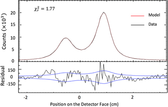
Figure 2. Representative titanium Kα profile used in calibrating the dispersion function. There is good consistency between our observed profile (black line) and previous characterisations (red line) from Chantler et al [9]. The raw data is partitioned into 550 x-axis points, each representing 0.1 mm. The counting error in each x-axis bin is shown by the blue line in the residual plot as is taken as  of the number of counts.
Download figure:
Standard image High-resolution imageThe crystal diffraction profile is defined by Moscurve theory which accounts for refractive index corrections, depth penetration of the wavefield into the crystal, and lateral shifts in position due to x-rays penetrating the crystal [24–26]. The Moscurve theory has been incorporated into a software package Mosplate, which has been used in several previous x-ray crystallography analyses [20, 22]. A Mosplate diffraction curve is illustrated in figure 3 of reference [20].
Mosplate calculates the energy of the diffracted photon from the position, x on the detector face, and the angle, θ of the detector arm; E = Emos(x, θ). The clinometers are calibrated to give a detector arm angle (Θ) as a function of recorded voltage, this takes the form of the sum between a shifted inverse sine function and a fifth order polynomial, giving a dispersion function:
where DU, DL, CC are the three clinometers referenced to a base clinometer value DB, and V is voltage.
The dispersion function calibrates the spectrometer and diffracting angle with respect to the clinometer voltages yielding accurate calibration of angle in arcseconds which then leads to accurate calibration of spectral energies in eV. Each dispersion function is fitted with the 312 energy centroids from the calibration profiles, this enables a very well defined functional with minimal uncertainty. An example for the CC dispersion function is shown in figure 3. Only the derived K , K
, K , and Kβ0 reconstructed peak positions are shown, 54 in total, rather than showing all 312 energy centroids for ease of viewing. We define the derived reconstructed peaks later.
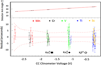
Figure 3. The dispersion function (equation (3)) for one of the clinometers (CC). The residual red-dotted line shows the calculated one standard error uncertainty for the fit. The residual plot also shows the one standard error uncertainties in the position for each transition centroid. Most lie within the one standard error envelope. The Sc Kβ positions are not used to fit the dispersion function, yet they lie within their standard error of the determined dispersion function. The dispersion function gives the detector angle for the Sc Kβ profile, and Mosplate theory is then used to obtain the final energy scale and profile.
Download figure:
Standard image High-resolution imageStatistical noise from these reference profile calibrations, represented by  , is small and robust and lies around the 0.5 meV level so is a minor contribution to the error analysis.
Once the dispersion function is defined, it is straightforward to input the recorded clinometer voltage for the Sc Kβ scans, and positions x from the detector into equation (4) to obtain energy scales for each of the three scans, and three dispersion functions. The consistency of these nine results are shown in figure 4.


Figure 4. The values for the peak value of Kβ0 for each of the scans for each clinometer with its respective one standard error uncertainty. The dotted red line shows the average value from the nine measurements.
Download figure:
Standard image High-resolution imageA major benefit of obtaining the energy of Sc Kβ1,3 using this method, as opposed to our earlier work on Sc Kα1,2 [20], is that the energy and detector arm angle are similar to that of the Ti Kα1,2 calibration line so that no extrapolation of the dispersion function is necessary. This reduces the overall uncertainty in this experiment by 0.001 eV (0.5 ppm), as it reduces the error associated with fitting the dispersion function from 0.006 eV to 0.003 eV (compare table 2 of this work to table 1 of [20]).
Table 2. The error budget for the reported Sc Kβ0 peak energy. The source of component contributions are detailed further in [20]. Individual independent contributions are summed in quadrature to yield the total estimated standard error.
| Error source | One standard error σse |
|---|---|
| Total Sc Kβ1,3 for E(Kβ0) | 0.0092 eV (2.1 ppm) |
| Sc Kβ1,3 counting statistics | 0.005 eV (1.1 ppm) |
| Sc Kβ1,3 clinometer voltage | 0.004 eV (0.9 ppm) |
| Variance, scatter and determination of the dispersion | 0.003 eV (0.7 ppm) |
| function including uncertainty of calibration lines and | |
| statistics on reference spectra | |
| Total geometry | 0.0052 eV (1.2 ppm) |
5. The detector x-axis dispersion function and error analysis
Some detectors, such as the one used in a recent investigation into copper K transitions [10], scan across angle continuously, taking readings for the count-rate as a function of angle only. Our method leaves the detector arm at a constant angle throughout the measurement for each scan of a profile. Therefore, to obtain a value in angle only, to be used in the dispersion function (equation (3)), we also had to define a dispersion function across the face of the detector. There would be three of these x-axis dispersion functions for each clinometer. The dispersion function in the x-axis ensures the linearity of our detector and leads to a more accurate final θ-axis calibration. An example for the x-axis dispersion function is shown in figure 5.

Figure 5. The x-axis dispersion function for one of the clinometers (CC). The residual red-dotted line shows the calculated one standard error uncertainty for the fit. The residual plot also shows the one standard error uncertainties in the position for each transition centroid. Most of the data points, with their individual fitting uncertainty, lie within the one standard error envelope. The Sc Kβ positions are not used to fit the dispersion function, yet they lie within their standard error.
Download figure:
Standard image High-resolution imageThere are four dominant sources of error for this experiment: the counting statistics for Sc Kβ1,3; the clinometer voltage uncertainty on Sc Kβ1,3; the uncertainty from fitting the dispersion function; and the geometric uncertainties. Each individual profile used for calibration has its counting statistic and clinometer voltage uncertainty—these are carried through to the total uncertainty of the dispersion function. The parameters (Pi) are calculated via the Levenberg–Marquardt algorithm which returns the uncertainty of the fit with the diagonalised covariance matrix. The total uncertainty from geometry comes from the quadrature sum of the uncertainty that each component has in the Mosplate calculations, following figure 1. Table 2 presents our final error budget of the reconstructed peak value. The individual components have their individual uncertainties which come from the quadrature sum of this error, and the fitting of the five Voigt functions to the profile.
A robustness investigation has been performed using a variety of input calibration profile sets. These have ranged from including only one Kα1,2 profile per calibration element; only Kβ1,3 profiles; or only profiles which fall on the right-hand side of the detector. Our result is not affected by more than 1σ by any choice of the calibration set. A selection of these different calibration sets is illustrated in table 1.
Also included in the robustness investigation is the result if we calibrate including additionally the three Sc Kα profiles (second row of table 1). The reported result is identical, the parameters Pi in the dispersion function (equation (3)) are unchanged; however, the uncertainty of the dispersion function reduces from 0.0031 eV to 0.0027 eV. This corresponds to a reduction in uncertainty for the total error only at the fourth decimal place (0.1 meV level).
Further consistency is tested when comparing the three clinometers and three separate scans of the Sc Kβ profile. These nine independent measurements show remarkable consistency, with all values within one standard error of another (figure 4).
6. Results
Our characterisation of the Sc Kβ profile is reported in table 3, with a plot of the model fitted to one set of data in figure 6. The resolution in our detector allows us to obtain values for the individual components—this was not possible for the earlier experimental data [8]. The Kβ peak position is always significantly affected by the amount of broadening present in the data. We report the peak energy Kβ0 of the reconstructed characterisation rather than the raw data. The characterisation, without Gaussian broadening, is shown in figure 7 along with the results of peak energy and FWHM.
Table 3. Voigt profile component fit for Sc Kβ. Numbers in parentheses are one standard error uncertainties. The common Gaussian width is 1.97(15) eV, and the constant background count is 473(14).  . The Lorentzian width of the full profile is 2.00(9) eV.
| Peak i | Centroid Ci (eV) | Lorentzian FWHM Wi (eV) | Integrated area Ai |
|---|---|---|---|
| βa | 4460.972(5) | 1.22(11) | 0.530(11) |
| βb | 4459.841(14) | 1.58(27) | 0.234(12) |
| βc | 4458.467(20) | 2.51(31) | 0.149(21) |
| βd | 4455.979(54) | 4.64(52) | 0.043(9) |
| βe | 4463.544(54) | 2.10(45) | 0.042(10) |

Figure 6. Characterisation of a spectrum of Sc Kβ using five Voigt profiles (table 3). Each data point represents a bin width of 0.016 eV. The counting error is shown by the blue line in the residual plot, as in figure 8.
Download figure:
Standard image High-resolution image
Figure 7. Characterisation of the same Sc Kβ profile with the Gaussian width removed—the reconstructed spectrum. The derived peak position, Kβ0, is 4460.845(9) eV with a Gaussian FWHM of 1.97(15) eV. The Lorentzian FWHM is 2.00(9) eV.
Download figure:
Standard image High-resolution imagePrevious relative characterisations use six profiles to characterise their spectra [15, 18]; however they have a high energy sixth profile for a satellite roughly 20 eV greater than the peak, which is beyond the range of our detector setting; therefore our use of five Voigt profiles is fully consistent with the other relative measurements for the spectral range. We compare the three characterisations of Sc Kβ from [15, 18] and this study in figure 8 and table 4, showing significant profile discrepancies for the three characterisations.

Figure 8. The three characterisations of Sc Kβ from [15, 18] and this study. The Gaussian width was a free parameter in each fit. For this data set, our new characterisation improves upon the earlier characterisations. The dominant errors of the previous relative measurements was the energy offset and scale.
Download figure:
Standard image High-resolution imageTable 4. Comparison of component centroids and parameters of this investigation (table 3) with those of Ito et al [18] and Anagnostopoulos et al [15]. Ito et al do not supply their individual component widths, only the widths of the reconstructed Kβ1 and Kβ3 profiles, irrelevant for this comparison. The component differences are huge, with energy offsets up to 10σse; much greater than the combined uncertainty from each experiment. This is due to the inconsistency or non-convergence of parameterisation of K-series x-ray spectra, including possible discrepancy of structure due to experimental conditions. A reconstruction of the individual data using these other characterisations gives a higher  for the earlier parametrisations, as shown in figure 8. Furthermore, we have not included a sixth high energy satellite (15 eV higher than the next highest energy component) that Anagnostopoulos et al and Ito et al include. Our detector does not record this higher energy regime, and the high energy component has no effect on the region of the main profile as discussed here.
| Peak i | Centroid Ci (eV) | Lorentzian FWHM Wi (eV) | Integrated area Ai |
|---|---|---|---|
| Comparison to Ito et al [18] | |||
| βa | 0.000 | NA | 0.229 |
| βb | −0.279 | NA | −0.013 |
| βc | −0.449 | NA | −0.248 |
| βd | 7.156 | NA | 0.006 |
| βe | −1.16 | NA | 0.024 |
| Comparison to Anagnostopoulos et al [15] | |||
| βa | 0.000 | 0.18 | 0.25 |
| βb | −0.201 | −0.27 | −0.066 |
| βc | 0.085 | −1.09 | −0.091 |
| βd | 3.307 | −11.85 | −0.097 |
| βe | −1.008 | −0.89 | 0.012 |
The component discrepancies in table 4 are much greater yet the characterisations are quite distinct. Of course these other characterisations were relative fits, and indeed the largest errors of these characterisations are the energy offset and scale. Fits were made allowing an offset of energy from the relative fits to align the peak more closely with the experimental data. Naturally this reduced the discrepancies of the relative fits yet the  was still significantly higher: 3.04 and 1.46 respectively. This highlights the value of a consistent paradigm across atomic spectral research, especially for locating and understanding satellite lines or comparisons with theory.
7. Measures of central tendency
Our discussion has focussed on the determination of the reconstructed characterisation peak energy E(Kβ0) as done by many previous authors for different transition metal characteristic profiles. Different measures of central tendency and experimental or theoretical results must be compared on a similar basis, with correction for additional or reduced broadening between experiments. These different measures are presented in table 5 for the current experimental profile and data. The uncertainty in them is generally identical to that of the derived reconstructed peak energy, since the correlations apply similarly. However, the component energy E(Kβa) is better defined as it only involves one centroid component. It is unclear if that relates exactly to the theoretical E(Kβ1) but it is certainly a good approximation.
Table 5. Different energy measures for our Sc Kβ profile based on different measures of central tendency and of characterisation of the profile position.
| Measure of central tendency | Symbol | Broadening (eV) | This experiment (eV) |
|---|---|---|---|
| Centroid of dominant component | E(Kβa) | 0 | 4460.972(5) |
| Reconstructed peak | Kβ0 | 1.22(11) | 4460.845(9) |
| Peak of the raw profile | Kβpeak | 1.22(11) ⊗ 1.97(15) | 4460.783(9) |
| Centre of mass | KβCoM | 10+ | 4460.493(9) |
The peak position shifts down in energy as the instrumental broadening increases, from an ideal limit near E(Kβ1) to the other ideal limit for a low resolution detector of E(KβCoM). This is a shift of 0.479 eV or much larger than the uncertainty for a well-defined peak measure. This is a clear example of why the peak position per se is not portable. However, the intrinsic peak, calibrated absolute energy and profile can be portable. Compared with our reported defined Kβ0 position, the shift for a typical low-resolution solid state detector KβCoM is a very significant 0.352 eV (table 5).
This encompasses the key issue in comparing the most current empirical and theoretical energy measurements. Bearden gives the peak of the profile, with an unknown Gaussian broadening [8], while Deslattes et al give the centroids of the two most dominant components with no widths [6]. Neither of these are sufficient characterisations to represent the spectra or structure. Deslattes et al give the component energies of 4462.93(80) eV and 4461.16(80) for Kβ1 and Kβ3 respectively. To reconstruct a peak energy or spectral profile, the widths and amplitudes must be known. One could introduce amplitudes calculated from the transition probabilities given in another source, such as the LLNL Evaluated Atomic Data Library [27], with natural linewidths calculated from emission rates from e.g. Scofield [28–30]. As mentioned, scandium is largely reported as an atom in theoretical calculations, with many factors such as electron correlation effects, solid-state effects, and shake effects left out of computations. We are interested in comparing the centroid energies, more than comparing calculated widths and amplitudes, we therefore compare using the theoretical component energies from Deslattes et al and our own observed empirical linewidths and amplitudes. Therefore, we provide the widths and relative amplitudes of our observed Kβa and Kβb components for the theoretical comparison with Kβ1 and Kβ3 components, namely 1.22 eV and 1.58 eV for widths and 0.69 and 0.31 for relative amplitudes, respectively. This gives a reconstructed Kβ0 peak energy of 4462.59 eV. The uncertainty of this value is the quadrature sum of our uncertainties and those of Deslattes et al dominated by the uncertainty of [6].
We may now investigate consistency and functionality of reported energies, summarised in table 6.
Table 6. Derived reconstructed peak energies for Sc  with experiment [8], and theory [6]. Numbers in parentheses are one standard error uncertainties. The difference column shows the deviation from our own measurement in eV.
| Reference | Sc  peak position (eV) peak position (eV) | Difference (eV) |
|---|---|---|
| This work | 4460.845(9) | |
| Bearden [8] | 4460.44(47) | −0.405 |
| Derived from Deslattes et al [6] | 4462.59(80) | +1.745 |
The value we obtain for the centre of mass measurement is strikingly close (0.007 eV) to the energy reported by Bearden. The discrepancy between the two experimental results may be dominated by the limited resolution of detector technology of the earlier study. If that is true, then the discrepancy reflects the lack of portability of the peak position in general; and it also reflects the real differences between our reporting of the reconstructed peak energy compared with a low resolution peak energy of the centre of mass.
The reconstruction of a peak energy for Deslattes et al has shifted the energy from Kβ1 to Kβ0 by −0.34 eV, which has reduced the overall discrepancy from 2.085 eV to 1.745 eV. However, this still stands as a significant discrepancy.
The experiment was made on high purity metal foils and the theoretical computation is on an isolated atom involving localised atomic initial and final states. Clearly solid state effects change the spectral profile of characteristic radiation and the Fermi level is strongly affected by bonding and ionisation state of the local atom. No literature has brought out explicit spectral shifts of a metal system compared with an isolated atom (to date) in the x-ray regime. To first order the ionisation state is zero in both cases like that of a neutral gas, so the main impact is expected to be in the valence orbitals and hence in the spectral contributions from high-level double satellites, which are very small [31]. Satellite structure in such systems is known to evolve from edge-excitation to the impact or sudden approximation [13, 14]—all these experiments were performed in the impact approximation.
Hence the metal system in the x-ray regime is an ideal testing ground for comparison of characteristic spectral profiles with atomic theory [32, 33]. Yet the significant discrepancy remains. This highlights the need for new calculations to be performed with a significantly smaller uncertainty to rigorously test the best current atomic theory and QED calculations [31]. More extensive theoretical investigation, possible with new computational software and power, is called for.
8. Radiative Auger satellite (RAS) analysis
As well as the effect of satellite profiles in the spectrum caused by shake events, the shape of the Kβ line may be influenced by radiative Auger satellites (RAS). These are rarely fitted to K series spectra as it is believed their amplitude is not significant. Indeed, RAS profiles have never been fitted to a Sc Kβ profile. However, the process is quite a significant contribution to the profile and especially to the profile asymmetry and it is observable in numerous spectra [34]. Hence neglect of this will prevent portability and transferability of reference standards and interpretation of the physics. It is unwise to ignore this phenomenon. A RAS profile has been characterised (approximated) by the following equation for intensity [35]:

where I is intensity, d, w are two width parameters, and E0 is the centroid. In table 7 we present the centroids, widths, integrated areas, of each of the five observed Voigt profiles, as well as the relevant parameters for the RAS satellite. The RAS profile and new components from table 7 are shown in figure 9. The background count has been significantly reduced and the low energy tail is larger due to the RAS profile. Importantly, the radiative Auger effect (RAE) well represents the tail asymmetry observed and observable in most spectra, and which is otherwise represented by an unphysical and extremely broad symmetric profile component Kβd. After including the dominant RAE, all component widths are dramatically reduced both to more physical values and towards some more ideal and valid resolution function. The new Kβd is at lower energies and is less extended and likely represents a limitation of the chosen functional for RAS. The functional form used here is common in the literature but is not fully justified.
Table 7. Voigt profile component characterisation for Sc Kβ now including an approximate form for the RAE profile. Numbers in parentheses are one standard error uncertainties. The common Gaussian width is 0.55(12) eV, and the constant background count is 259(11). The RAS profile has parameters d = 0.200 and w = 1.22.  .
.
| Peak i | Centroid Ci (eV) | Lorentzian | Integrated area Ai |
|---|---|---|---|
| FWHM Wi (eV) | |||
| βa | 4461.080(5) | 0.60(11) | 0.386(11) |
| βb | 4460.201(14) | 0.78(27) | 0.272(12) |
| βc | 4458.964(20) | 1.38(31) | 0.182(18) |
| βd | 4451.038(54) | 3.51(52) | 0.065(9) |
| βe | 4463.405(54) | 1.71(45) | 0.061(10) |
| RAS | 4460.500(0) | N/A | 0.033(9) |

Figure 9. Characterisation of the same spectrum as in figure 6 but with an RAS component fitted. Each data point represents a bin width of 0.016 eV with the counting 1σ error shown by the blue line in the residual plot.
Download figure:
Standard image High-resolution image
Whilst the RAE is the weakest of the components in the range of the fit, it has an extended low energy tail. The accuracy of the component energies is largely unchanged, yet their values shift by relatively large amounts to accommodate the asymmetry of the RAE.
The existence of RAS is well known and documented. The goodness-of-fit measure ( ) has grown slightly, due purely to the extra peak parameters decreasing the number of degrees of freedom. However it is clear that including the RAS profile for the full characterisation is important and makes all parameters more physical and more portable. As detector technology improves and measurements become more well resolved, the RAS profile will become increasingly important. Therefore our implementation is necessary. More theoretical and experimental work is demanded on this important issue. In particular the resulting Kβ ratios appear implausible given other research. Hence here we raise the complex issue and look forward to more work on the area.
This final characterisation to 2.1 ppm is the best so far attempted and has an absolute accuracy based upon the experimental data and does not depend in any way on theoretical assumptions or approximations. It is portable as it stands. However, some aspects of the parametrisation remain empirical, so an individual component certainly does not relate directly to a single theoretical transition—though it is quite a good match for the two dominant diagram lines. This analysis also does not depend upon the interpretation uncertainty of theory, but is an experimental measurement; nor does it depend upon the experimental lack of resolution, since it represents the structure of the observed profile.
9. Discussion
The methods used in obtaining the absolute energy for the Sc Kα and Kβ profiles discussed here and by Dean et al [20] are highly versatile and robust. Through careful selection of the diffracting crystal, and the calibration transitions, it is possible to perform the same analysis for any emission spectra with energy ranging from as low as 500 eV and up to 30 keV, and achieve accuracies down to the 0.01 eV range as seen above.
With the same experimental analysis performed at an electron-beam ion-trap (EBIT), there is great potential for QED measurements to be reduced in uncertainty by a factor of 10 which will provide much stronger constraints on QED measurements from atomic physics. This is an argument for the value of the technique—of course the investigation of any quantum system must be calibrated by reference lines such as this across the same energy range, whether with a single point or multiple point calibration. For example, two recent studies showed measurements of He-like Ti-ions to 15 ppm accuracy [3, 36]. The transition lines considered by Payne et al are around 4950 eV which is similar energy range to Sc Kβ, therefore making our analysis easily transferable. Their uncertainty of 15 ppm comes largely from the uncertainty in the dispersion calibration function (table 2) which is 10 ppm. This factor could be greatly reduced using our described analysis. Another uncertainty comes from the EBIT data which could also be reduced to below the 10 ppm range.
Advanced detector studies including searches for dark matter candidates could be made with this careful analysis, since candidates are expected to make subtle shifts to spectral profiles. Of course, this study would only directly encourage measurements across the same energy range, in the x-ray regime. Several astrophysical groups have also requested new experimental parameters for their stellar and interstellar spectral surveys, which indeed could have bearing on quests for the constancy of the speed of light and the fine structure constant for example.
10. Conclusion
The consistency with previous experiments and theory is clear, representative of the reliability of curved crystals in diffraction experiments for spectrometry. Our new uncertainty of 2 ppm further demonstrates the utility of curved crystal diffraction for spectrometry, as well as the robustness of our method to quantify and correct for geometric uncertainties. It is important to investigate whether a modern theoretical calculation, with smaller error bars, might resolve the discrepancy. The experimental and analytical techniques that have been demonstrated, can be used to explore other important spectral features, polarisation, plasma excitation, highly charged ions, anomalies of few-electron x-ray tests of QED and astrophysical and particle searches. In particular, future experimental and reference work should carefully consider any RAE profiles and contributions to avoid significant systematic error.
The Sc Kβ1,3 spectrum has not been subject to an absolute energy calibration for over 50 years. This work reports values almost 30 times more accurate than the previous reported value from the literature [8]. Additionally, if the interpreted energy and uncertainty of the experimental result reported is valid [6], then the improvement of this new measurement is about a factor of 50. Further, the accuracy of this result compared with the current theory is improved by a factor of almost 100 [6], enabling novel relativistic quantum mechanical theory to test consistency with experiment. The characterisation of five Voigt profiles is highly accurate and gives insight into asymmetries and the ratio of line intensities. The characterisation of component peaks is essential for transferability of standards and for detailed investigation of relativistic quantum mechanics.