
Abstract
The magnetic field is a key feature that distinguishes magnetron sputtering from simple diode sputtering. It effectively increases the residence time of electrons close to the cathode surface and by that increases the energy efficiency of the discharge. This becomes apparent in high power impulse magnetron sputtering (HiPIMS) discharges, as small changes in the magnetic field can result in large variations in the discharge characteristics, notably the peak discharge current and/or the discharge voltage during a pulse. Here, we analyze the influence of the magnetic field on the electron density and temperature, how the discharge voltage is split between the cathode sheath and the ionization region, and the electron heating mechanism in a HiPIMS discharge. We relate the results to the energy efficiency of the discharge and discuss them in terms of the probability of target species ionization. The energy efficiency of the discharge is related to the fraction of pulse power absorbed by the electrons. Ohmic heating of electrons in the ionization region leads to higher energy efficiency than electron energization in the sheath. We find that the electron density and ionization probability of the sputtered species depend largely on the discharge current. The results suggest ways to adjust electron density and electron temperature using the discharge current and the magnetic field, respectively, and how they influence the ionization probability.
Export citation and abstract BibTeX RIS

Original content from this work may be used under the terms of the Creative Commons Attribution 4.0 license. Any further distribution of this work must maintain attribution to the author(s) and the title of the work, journal citation and DOI.
1. Introduction
For over four decades the magnetron sputtering discharge has been applied successfully for deposition of thin films and coatings with applications in various fields in both academia and industry [1, 2]. The magnetron sputtering discharge is a magnetically enhanced glow discharge where the residence time of the electrons in the vicinity of the cathode target is extended by the presence of a static magnetic field. In the planar circular configuration, this is done by concentrically placing a central cylindrical magnet and an outer edge ring magnet behind the cathode target, with anti-parallel magnetization. In the presence of such a magnetic field, the discharge voltage is lowered, the working gas pressure can be decreased, and the deposition rate is substantially increased, compared to non-magnetized dc diode sputtering [3, 4]. In this planar circular magnetron configuration, the static magnetic field is arranged in such a way that the electrons drift azimuthally. The magnetic field strength is typically in the range 20–50 mTesla [3], so the electrons are magnetized, while the magnetic field does not influence the ion trajectories directly [5].
The magnetic field strength and the degree of magnetic unbalance have a significant influence on the discharge current and/or the discharge voltage. This is particularly true for the high power impulse magnetron sputtering (HiPIMS) discharge, in which small changes in the magnetic field strength and/or degree of unbalance can give strong variations of the discharge current waveform and the discharge voltage [6–8]. For a fixed discharge voltage, an increased magnetic field strength leads to an increased peak discharge current. For a fixed peak discharge current, increasing the magnetic field strength decreases the discharge voltage [8]. The degree of magnetic unbalance also influences both the discharge voltage and current, but these effects are less well studied.
The key to understanding the changes in the discharge voltage and current waveforms lies in how the discharge voltage  is split between the cathode sheath and the ionization region (IR). The presence of a transverse magnetic field enables a potential drop to exist outside the cathode sheath [9–12]. In sputtering magnetrons, this potential outside the sheath is denoted as
  , where the subscript IR signifies the ionization region in the vicinity of the cathode target. The discharge voltage thereby falls over the cathode sheath and the IR, i.e.
  , where
  is the sheath potential drop. Unlike non-magnetized dc diode sputtering discharges, which are primarily maintained by ion-induced emission of secondary electrons accelerated in the cathode sheath [1, 13], the addition of a potential
  across the IR enables Ohmic heating of the electrons [14], which describes locally absorbed power by the electrons within the IR. In magnetron sputtering discharges, this results in an energy gain by electrons that are moved across a fraction of the potential drop
  .
.
Ohmic heating is believed to be the dominating electron power absorption mechanism of HiPIMS discharges [15, 16]. More importantly, though, it is accompanied with less ion acceleration, compared to sheath energization. This is because the current in the IR is composed of both ions and electrons in equal shares, compared to the sheath, where the current is composed mostly of ions, while electrons make up only a few % due to an effective secondary electron emission yield of around 0.05 [16]. Therefore, the total power that is necessary to heat electrons by Ohmic heating is only 10%–20% compared to the power needed to heat electrons by the same amount in the sheath [16]. Total power here means the power dissipated by both electrons and ions. The result is that for discharges with a higher fraction of Ohmic heating over total electron heating (Ohmic heating plus sheath energization), the same discharge current can be maintained at a lower discharge voltage. The discharge becomes more energy-efficient.
There are indications that the ratio of Ohmic heating to sheath heating changes depending on the magnetic field configuration. Mishra et al [17] observed a decrease in  with decreasing magnetic field strength by emissive probe measurements. Computational modeling of HiPIMS discharges show that a weaker magnetic field results in weaker Ohmic heating in combination with a decreasing voltage fraction across the ionization region, i.e.
  decreases with decreasing magnetic field strength [16]. Despite these results, there is still a limited understanding of to what extent the magnetic field influences changes in Ohmic heating within the IR.
In the present work, therefore, we address the challenge on how the magnetic field affects internal discharge parameters, like the electron density and electron temperature, how it changes the relative contribution of each of the two electron power absorption mechanisms, Ohmic heating and sheath energization, and how these variations in the discharge properties in turn influence a key property of a HiPIMS discharge, the probability of target species ionization. This is done by modelling several HiPIMS discharges. The HiPIMS discharges are taken from the experimental studies of Hajihoseini et al [8] who studied magnetron sputtering discharges with varying magnetic field configurations. The modelling is done using an updated version of the ionization region model (IRM) [18, 19]. The IRM is a time-dependent volume-averaged plasma chemical model of the dense plasma in the ionization region adjacent to the cathode target racetrack [3, 4]. The experimental discharge current–voltage waveforms used to lock the IRM are here extended to include the ionized flux fraction [20] for each of the investigated discharges. Also, the IRM is improved by including consideration of an afterglow [18], and a revision of electron impact excitation and ionization cross sections [19]. These changes make it possible to better lock the IRM and thereby establish key trends in discharge parameters versus magnetic field configuration with smaller error bars on all calculated parameters.
In section 2, we shortly describe the setup of the experimental discharges and the modelling of these discharges using the IRM. Section 3 discusses the results and is split up into discussing the influence of the magnetic field configuration on the electron density (section 3.1), on the electron heating and the corresponding electron temperature (section 3.2), and the combined effect of density and electron temperature on the ionization probability of target species (section 3.3). A summary is provided in section 4.
2. Experimental and model description
The modelling done here is based on experimental discharges analyzed by Hajihoseini et al [8], in which the focus of the study was on how the magnetic field strength and degree of unbalance influence the deposition rate and the degree of ionization in the flux of film forming species towards the substrate. In the studied discharges the working gas pressure was kept constant at  Pa, the pulse length at
  µs, and the average discharge power at
  = 300 W, as the magnetic field strength and degree of unbalance were varied.
2.1. The electron-confining magnetic field of the magnetron assembly
The magnetron assembly used for the discharges in Hajihoseini et al [8] had an adjustable confining magnetic field. It was a planar circular magnetron assembly with a 4 inch target diameter and consisted of a center (C) and an annular edge (E) magnet pack. The distance of each magnet pack from the target rear could be adjusted. The magnetic field configurations obtained in this way were denoted C E
E where
where  and
and  were distances in mm measured from the position closest to the rear of the target. The definition of
  and
and  is shown schematically in figure 1. E.g. the magnetic configuration C0E5 meant that the central magnet was positioned closest to the rear of the target, while the annular edge magnet was 5 mm away from the position closest to the rear of the target [8]. The magnetic field configurations that could be obtained by the magnetron assembly described above, were all of unbalanced type II based on the definition of Window and Savvides [21].

Figure 1. Schematic drawing of the magnetron assembly with definitions of the parameters  and
and  , and the distance coordinates
  and
and  for the central (C) and the annular edge (E) magnet with respect to their closest position to the rear of the target, respectively.
Download figure:
Standard image High-resolution imageThe magnetic field configurations were characterized in Hajihoseini et al [8] by two magnetic field parameters determined from mapping the magnetic field  above the target surface: (a) the magnetic field strength at 11 mm above the racetrack,
  , and (b) the distance to the magnetic null point measured from the target surface,
  . The magnetic field parameters
  and
and  are defined in figure 1.
Instead of using the magnetic field parameters  and
and  , we here use the sum of the two distances of the central and the edge magnet from the rear of the target to describe the magnetic field. We denote this constructed parameter
  . Table 1 gives the values of the three parameters
  ,
,  , and
, and  for the seven studied magnetic field configurations. The reason for using
  rather than the often used or 'classical' magnetic field parameters
  and
and  , is that this parameter captures rather well similarities between discharges having very different magnetic field configurations. As shown below, certain discharge parameters exhibit smooth trends with variations of
  and discharges with the same
  show similar values of these parameters. It is therefore an empirically verified similarity parameter. We also note that
  can remotely be related to the measured magnetic field parameters. It is intuitively clear, that by moving any of the two magnet packs away from the rear of the target, the contribution to the magnetic field above the target is reduced. Note that this is not a localized change of the magnetic field strength but it is rather an integral change of the magnetic field strength in the whole volume of the IR. Figure 2 shows the relation of
  to the measured parameter
  . The dashed line is a linear fit to the three configurations where both the magnet packs are moved together (filled blue triangles). For these configurations there is an almost linear trend of decreasing
  for increasing
  . However, the other configurations, in which the two magnets are at different distances from the target, give a considerable scatter around this trend. Note, that the discussion here is based on the stationary magnetic field that is due to the permanent magnets (the magnet packs). It has been demonstrated through measurements that the magnetic field can be deformed by the azimuthal currents (Hall drift and diamagnetic drift) in the discharge, and changes of up to 1–2 mTesla have been reported [22]. The deformation depends on the spatial location and appears to be up to roughly 10% of the magnetic field just above the racetrack region.

Figure 2. The magnetic field strength  , measured 11 mm above the racetrack, versus
  . The dashed line is a linear fit through the three configurations where the magnetic packs are moved together, C0E0, C5E5, and C10E10 (filled blue triangles).
Download figure:
Standard image High-resolution imageTable 1. The three magnetic field parameters  ,
,  , and
, and  , which can be used to describe a magnetic field configuration, for the seven different studied magnetic field configurations. The values for
  and
and  are taken from Hajihoseini et al [8].
| Magnetic field configuration |
 (mm) (mm) |
 (mT) (mT) |
 (mm) (mm) |
|---|---|---|---|
| C0E0 | 0 | 23.3 | 66 |
| C0E5 | 5 | 21.7 | 70 |
| C0E10 | 10 | 21.3 | 74 |
| C5E0 | 5 | 18.1 | 53 |
| C5E5 | 10 | 16.1 | 59 |
| C10E0 | 10 | 13.7 | 43 |
| C10E10 | 20 | 11.1 | 52 |
The choice of magnetic configuration has a very large impact on the discharge properties. For example, between the two extreme configurations C0E0 to C10E10, the peak discharge current  for the discharges run in fixed voltage mode decreases from 76 A to 12 A. For the discharges run in fixed voltage mode, the discharge voltage
  increases from 510 V to 660 V between the configurations C0E0 and C10E0. A detailed description of these changes are given by Hajihoseini et al [8].
2.2. Discharge modelling
We use the IRM to obtain a set of internal discharge parameters that are relevant for our discussion on the discharge physics. The IRM is a global plasma-chemistry model based on energy balance and particle balance and was developed to improve the understanding of the operation of HiPIMS discharges [16, 23]. It models the volume reactions inside the IR and the species interactions with the target surface, as well as the fluxes in and out of the IR such as the sputter flux into the IR and the out-diffusion of working gas and target species [16, 24]. As the IRM is semi-empirical, it needs experimental input. As in earlier studies [16, 18, 19, 25], this input was the measured discharge current and voltage waveforms as well as the ionized flux fraction measured above the IR. All of these measured values are available for the discharges described in section 2.1.
The IRM gives access to internal discharge parameters that are usually not easily accessible by experiments. Here, in particular, we discuss a sub-group of six internal parameters that are involved in the energy balance in the discharge, namely the discharge voltage  , the sheath potential
  , the potential drop over the ionization region
  , the temperatures of the cold and hot electron groups
  and
and  , respectively, and the power fraction of Ohmic electron heating over the total power to the electrons
  . Note that the IRM is a global model which uses the approximation that the internal discharge parameters are homogenous inside the considered IR volume. It therefore provides spatially averaged internal discharge parameters that may, in reality, be superimposed by spatial and temporal variations caused by e.g. instabilities such as spokes [26]. The use of a global model also implies that the magnetic field cannot be taken into account explicitly. The magnetic field, in reality, is strongly varying in magnitude and direction within the IR of a magnetron sputtering discharge, which is incompatible with a global approach of plasma parameters being homogeneous in the IR. Therefore, the magnetic field is not modelled explicitly, but rather taken into account indirectly, by using experimentally determined parameters measured under different magnetic configurations, e.g. the ionized flux fraction and the discharge current waveform to fit the model to the discharge.
The IR volume lies above a disc cathode target. It is approximated by a torus with a rectangular cross-section with inner and outer radius r1 and r2 and a height  , where z1 is the sheath width, sitting above the racetrack. We lack the data to determine if the height of the IR changes with the magnetic field configuration. Therefore, the assumption of a constant IR volume may not be valid. However, we will show that the discharge parameters obtained from the IRM are largely insensitive to changes in the IR volume. We therefore, in the following, report the values for an IR of
  mm,
mm,  mm,
mm,  mm and
  mm, as used in earlier studies using this experimental data set [18, 19, 25]. At the same time, we add uncertainty bars to each data point that give the uncertainty range if the height L of the IR is changed by
  %.
%.
3. Results and discussion
The discharges described in section 2 were controlled by keeping the peak discharge current constant (fixed current mode) or by keeping the discharge voltage constant (fixed voltage mode) while the magnetic field configuration was varied. At the same time, the pulse repetition frequency for all discharges was adjusted in order to keep a constant average power [8]. As the IRM models only single pulses, the pulse repetition frequency is not explicitly modelled. Therefore, for the modelled discharges, there is only one control parameter, that is the peak discharge current for the discharges operated in fixed current mode or the discharge voltage for the discharges operated in fixed voltage mode. Keeping one or the other of these two adjustable control parameters constant reveals different aspects of the discharge physics, as discussed in the following.
In section 3.1 we begin our analysis by studying how the peak discharge current influences the electron density  in the IR. This is followed by unravelling the reasons for the variations of the discharge voltage in the case of the fixed current discharges and the peak discharge current in the case of the fixed voltage discharges. To explore this, in section 3.2, we look at how a sub-group of internal discharge parameters varies with the magnetic field. The reason for using a HiPIMS process for thin film deposition is the enhanced probability of target species ionization. In section 3.3, we therefore discuss the variations of the probability of target species ionization in view of the variation of the internal discharge parameters discussed in the preceding sections.
3.1. Influence of the magnetic field and the discharge current on the electron density
Let us first analyze how the discharge current influences the electron density  . Figure 3 shows the temporal evolution of the discharge current and the electron density
  within the IR, as determined by the IRM for four cases: two in fixed peak current (40 A) mode and two in fixed voltage (625 V) mode. We see that the evolution of the
  (t) and
  (t) curves follow each other rather closely during the entire pulse-on time. They can be approximated quite well by

where  is in (A) and
  is in (m−3). An evaluation for all the experimental data (not shown) shows that this approximation holds equally well independent of the magnetic field configuration, the applied discharge voltage and current, and during all times within the HiPIMS pulse. Using the surface area of the target,
  m2, equation (1) can be expressed in terms of current density,
  (A m−2), averaged over the entire target surface
  ,
,

Figure 3 shows that after the end of the pulse, the discharge current rapidly drops to zero. The electron density decays more slowly, though. The trajectory of ions to the cathode target is not influenced by the magnetic field, but by a potential in the pre-sheath region that leads to ion back-attraction. When the pulse ends, ion back-attraction disappears, and the ions can freely leave to the diffusion region [15, 18]. We propose that the decay rate of the plasma density is determined by this ion loss. However, maintenance of quasineutrality demands that ions and electrons leave the magnetic trap region at the same rate. Consequently, the electrons easily leave the IR, at a rate limited to maintain quasineutrality, by motion along the magnetic field lines. The temporal evolution of the ion densities determined by the IRM for selected magnetic field configurations and discharge modes is shown in figure 4. In all cases the Ar+ ion has the highest density, the Ti+ density is always somewhat smaller, and the Ti2+ density is always at least an order of magnitude smaller. In fact, the highest Ti2+ ion density observed is 2.7% of the total ion density and is reached for the discharge run in fixed voltage mode with the magnetic field configuration C0E0. The Ti+ ions appear later than the Ar+ ions and the Ti2+ ions appear the latest. The decay rate of the Ti+ is faster than for the Ar+ ions.

Figure 3. Comparison between the temporal evolution of the discharge current and the electron density determined by the IRM for selected magnetic field configurations and discharge modes. Fixed current mode ( A) for configuration (a) C0E0, and (b) C10E0, and fixed voltage mode for configurations (c) C0E0 (
 A), and (d) C10E10 (
 A). In all cases the electron density follows closely the discharge current during the 100 µs HiPIMS pulse. Note that the scale for the discharge current
  and the electron density
  does not change between panels.
Download figure:
Standard image High-resolution image
Figure 4. The temporal evolution of the ion densities determined by the IRM for selected magnetic field configurations and discharge modes. Fixed current mode ( A) for configuration (a) C0E0, and (b) C10E0, and fixed voltage mode for configurations (c) C0E0 (
 A), and (d) C10E10 (
 A).
A).
Download figure:
Standard image High-resolution imageThe resemblance between the time-evolution of  and
and  during the HiPIMS pulse has been observed before experimentally by Held et al [27]. It can be understood by equalizing the discharge current with the ion current to the target. We note that at the target surface the discharge current density is usually normalized to the racetrack surface area
  . At the target surface the discharge current is mainly carried by ions from the IR, neglecting the contribution from secondary electrons, the current density is given by Huo et al [16]:
where k denotes the ion species (k = Ar+, Ti+, Ti2+), e is the elementary charge, and  is the time-dependent ion current to the racetrack. As ion species, here, we take Ar+, Ti+ and Ti2+, because these are modelled in the IRM. On the right hand side, ak
is the charge state of ion species k,
is the time-dependent ion current to the racetrack. As ion species, here, we take Ar+, Ti+ and Ti2+, because these are modelled in the IRM. On the right hand side, ak
is the charge state of ion species k,  is their density in the IR,
  is their loss time out of the IR, and βpulse is the probability of ion back-attraction to the target during the pulse [18]. The loss time for ion species k can be approximated by [16]
where  is the height of the IR above the sheath edge,
  is the potential drop over the IR and mk
is the mass of ion species k. Sheridan et al [28] argue that since electrons and ions are created at almost the same rate, their confinement time must be roughly the same and consequently
is the potential drop over the IR and mk
is the mass of ion species k. Sheridan et al [28] argue that since electrons and ions are created at almost the same rate, their confinement time must be roughly the same and consequently  , given that the magnetic geometry and the ionization profile remains fixed. We here note that we find the same proportionality in equation (4). We enter
  from equation (4) into equation (3), and move out constant terms from the summation, giving
Let us evaluate equation (5) for a 'typical ion, in a typical discharge'. From previous IRM runs, we know that βpulse lies in the range 0.87–0.93 [25] and we here use the mean value βpulse = 0.9. The value of  varies between 36 and 50 V for the present discharges (see figure 6(a) below). Here, we use a mean value of
  = 43 V. Furthermore, we replace all three ionic species by a single species with charge state
  which is justified because only a few percent (
 % of the ion density) of doubly charged ions (Ti2+) are present in the discharge (see figure 4). We also use a single value for the mass
  , where
  is the proton mass, which lies between the masses of argon
  and titanium
  . Moving out all constants from the summation in equation (5), and resolving
  to the left, yields
where  is in (m−3) and
  is in (A m−2) and where we have used the condition of quasi-neutrality to replace
  with
with  . Using
  with
with  m2 and
  m2 we obtain the relation between
  and the current density normalized to the entire target surface area,
This result for a 'typical ion, in a typical discharge' agrees well with the empirical approximation of equation (2). The small deviations in figure 3 from an exact proportionality between  and
and  can be understood from the variations of the parameters βpulse,
  , and mk
around the assumed typical values. Here, the slight deviation of the electron density from the discharge current for the discharge run in fixed current mode and using the magnetic field configuration C0E0 (figure 3(a)) compared to that with the magnetic field configuration C10E0 (figure 3(b)) are mainly due to a variation in
, and mk
around the assumed typical values. Here, the slight deviation of the electron density from the discharge current for the discharge run in fixed current mode and using the magnetic field configuration C0E0 (figure 3(a)) compared to that with the magnetic field configuration C10E0 (figure 3(b)) are mainly due to a variation in  . For the magnetic field configuration C0E0,
  = 50.5 V, and for the configuration C10E0,
  = 40.9 V (see figure 6(a)). This difference results in a 10% lower electron density for the configuration C0E0 compared to the configuration C10E0 in fixed current mode. Similarly, the discharges run in fixed voltage mode with the magnetic field configurations C0E0 and C10E10 clearly have a very different peak discharge current (
 A and 12 A, respectively) and, therefore, exhibit a different composition of the ion current at the target surface. Here, for Ar and Ti with very similar masses, the proportionality factor between
  and
and  changes only by
  % between the two extreme cases of a pure Ar+ current compared to a pure Ti+ current.
Measurements of the electron density in HiPIMS discharges have been made over the years. A compilation of peak electron densities normalized to the peak discharge current density (averaged over the entire target) for various HiPIMS discharges and target materials (Ti, Cu, Cr, Al, C, Ta, Nb, and W) has been made by Čada et al [29]. All discharges in that compilation were operated with argon as the working gas over a range of pressures (0.27–2.7 Pa) and it is found that with variations of the process conditions (pressure, target size, and target material), the pulse configuration, and the exact location of the probe measurement in the discharge,  varied in the range
  –
– (Am)−1 [29]. Our results (equation (2)) lie at the upper border of what has been observed experimentally, which may be explained by the measurements not being made close to the target, i.e. in the most intense part of the discharge, where probe measurements are typically difficult to do. The reported experimental electron densities are therefore often lower compared to the here-presented values from the IRM. Taking these experimental challenges into account, in general, the agreement between experiments and modelling seems acceptable. It suggests that the close link between the electron density and the discharge current is a fundamental relation with a validity that goes beyond the discharges under investigation here. It is therefore concluded that, for any given discharge current, neither the magnetic field strength nor the degree of magnetic unbalance has any significant influence on the electron density. The principal influence on the electron density is from the discharge current, and here the relation is a simple proportionality.
3.2. Influence of the magnetic field on the electron temperature and Ohmic heating
In the preceding section we have learned that, independent of both the magnetic field configuration and the time during the pulse, the electron density in the IR closely follows the discharge current. In our case this relation  is given by equation (1). The experimentalist can therefore select any desired electron density by adjusting the discharge current. The electron density is to a large extent determined by the rate coefficient for electron impact ionization, which in turn is determined by the electron temperature. The following section is therefore an analysis of how the electron heating and the electron temperature change with varying magnetic field configuration and discharge current.
Let us first discuss the two externally measured discharge parameters that are involved, the discharge voltage and current. Figure 5 gives the variations of discharge voltage and current with the magnetic field parameter  . Remember that the parameter
  is an empirical parameter that represents changes in the magnetic field configuration. Despite its ad-hoc nature and simplicity, it seems to capture quite well the essence of the magnetic field configuration. This can be seen by considering the trends in either fixed current mode or fixed voltage mode, where very different magnetic field configurations have a similar discharge voltage as shown in figure 5(a) and a similar discharge current as shown in figure 5(b), if the parameter
  has the same value. That applies to the magnetic field configurations (C0E5, C5E0) and (C0E10, C5E5, C10E0) with values of
  = 5 mm and
  = 10 mm, respectively. Keep in mind that the discharge voltage, the discharge current, and
  are experimentally determined parameters and independent of any model, which gives us confidence that the parameter
  carries a physical meaning.
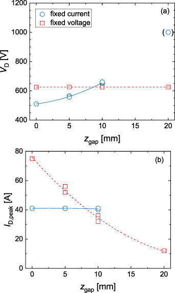
Figure 5. (a) The discharge voltage  , and (b) the peak discharge current
  , as a function of the empirical parameter
  for the discharges run in fixed current and fixed voltage mode. Note, that the data point in parenthesis indicates a lower boundary for the discharge voltage, as the discharge did not reach the required peak discharge current of 40 A at the maximum output voltage of the used pulsing unit. The lines are 2nd order polynomial fits to the data points.
Download figure:
Standard image High-resolution image
Figure 6. IRM-derived discharge parameters: (a) potential drop over the IR  , (b) cathode sheath potential drop
 , (c) temperature of the cold electron group, and (d) temperature of the hot electron group. The uncertainty bars indicate the range of parameters obtained by varying the IR height by
  %. The hot electron temperature does not depend on changes in the height of the IR. All parameters are averaged over the pulse length. The reported parameter values are averaged over one pulse.
Download figure:
Standard image High-resolution imageThere is in figure 5, both for the fixed current and for the fixed voltage cases, a common trend: for smaller values of  , the discharge delivers 'more current per voltage'. Huo et al [16] discuss the relation between discharge current, discharge voltage and magnetic field strength. They define an effective discharge impedance as
  , and report a decreasing
  with increasing magnetic field. Since a smaller
  is correlated to stronger magnetic fields (figure 1) this is consistent with our findings here: the discharges with a lower value of
  exhibit a lower effective discharge impedance
  . As an entry to the analysis below we can note that this is somewhat counterintuitive, since a stronger B-field leads to a lower electron mobility across the magnetic field lines [30, 31]. One could, therefore, expect that a higher discharge voltage would be needed to drive the electron current across a stronger magnetic field, and thus result in a higher
  . Let us call the observed opposite trend the 'apparent voltage paradox'.
For a deeper insight, we have from the IRM-runs extracted how four internal discharge parameters vary as functions of the magnetic field parameter  . The parameters that we will look at are the sheath potential
  , the potential drop over the IR,
  , and the temperatures describing the cold and hot electron groups
  and
and  , respectively. The trends of these parameters with
  are shown in figure 6.
The potential drop over the IR,  , as well as the cathode sheath voltage,
  , are presented in figures 6(a) and (b), respectively.
  shows quite a similar trend for the discharges run in fixed current and fixed voltage modes. In both cases, it decreases with increasing
  (which, again, is correlated to weaker magnetic fields). This observation is in line with experimental probe measurements by Mishra et al [17] who reported a smaller potential drop over the IR for weaker magnetic fields. For
  , the trends for the two modes are similar in the sense that both are rising, but they are dissimilar in strength. While the fixed voltage cases have only a small increase of
  , the fixed current cases show a strongly increasing
  , with increasing parameter
  . For both discharge modes, the
  curves in figure 6(b) strongly resemble the
  curves in figure 5(a). This is not the case for the
  curves. For the discharges run in fixed current mode,
  even shows the opposite trend: despite a rising discharge voltage in figure 5(a) with increasing
  ,
,  decreases as shown in figure 6(a).
The trends in  for both discharge modes are mimicked by the temperature of the cold electron group (compare figures 6(a) and (c)). This can be explained by Ohmic heating that depends on the potential drop over the IR,
  . Most of the power delivered to Ohmic heating is used to heat cold electrons, simply because they have a much higher number density compared to the hot electron group [19]. Similarly, the trends in
  for both discharge modes are mimicked by the temperature of the hot electron group (compare figures 6(b) and (d)). This observation can be explained by the hot electrons gaining their energy in the cathode sheath and that the energy gain corresponds to exactly the sheath voltage
  .
.
The coupling between the three discharge parameters  ,
,  , and
, and  can be understood as a combination of particle balance and energy balance. In order for the plasma to remain quasi-neutral, the loss rates of ions and electrons from the IR during the pulse have to be identical, the ions going mainly to the target and the electrons to the diffusion region. For simplicity we now consider the fixed current discharges only, and the effects of a decrease in the parameter
  . This scales approximately with a stronger magnetic field as can be seen in figure 2. The Pedersen conductivity governs the current along the axial electric field that is transverse to the magnetic field (electron cross-B), while the Hall conductivity determines the current perpendicular to both the magnetic and the electric fields [32, section 5.3]. For a stronger magnetic field, the electron Pedersen cross-B mobility decreases [30, 33], and a higher potential drop
  therefore becomes necessary to give the same electron cross-B drift speed towards the diffusion region. This higher IR potential drop is seen in figure 6(a), and it brings the energy balance into the picture because it increases the rate of Ohmic heating of electrons [16], and thereby gives a higher (cold) electron temperature
  , as can be seen in figure 6(c). This, in turn, reduces the need for a high ionization rate from the hot electron population. The fixed discharge current can therefore, at lower
  , be maintained at a lower sheath voltage, as seen in figure 6(b), and a lower hot electron temperature, as seen in figure 6(d).
Figure 7 shows the power dissipation channels for three fixed current discharges with different values of  . The surface area of the pies indicates the pulse power, i.e. the electrical energy dissipated during one pulse divided by the pulse length [34],
where  is the pulse length. One can see that most of
  , or
, or  %, is used to accelerate ions, mostly across the cathode sheath, and this power is finally dissipated in the target as heat. For the discharge with magnetic field configuration C0E0 (
 = 0), 7% of the pulse power is absorbed by the electrons and this fraction decreases for higher values of
  , indicating a shift to less energy-efficient discharges. In other words, for an increasing magnetic field parameter
  , more energy is spent on heating up the target.

Figure 7. Fractions of pulse power for fixed current discharges with different values of  that are used for ion acceleration (
 ), Ohmic heating (
 ), and sheath energization (
 ). The power (in (kW)) stated above each diagram is the pulse power
  defined in the text.
Download figure:
Standard image High-resolution imageThe parameter  can similarly be regarded as a measure for energy efficiency of a discharge. This is because a higher fraction of Ohmic heating over total electron energization
  will always have a lower
  because Ohmic heating of electrons is accompanied by less ion heating compared to sheath energization of electrons. This is the reason why both measures of efficiency, the fraction of total power that goes to electron heating, and the electron-energizing fraction of the power that goes to Ohmic heating,
  , are equivalent.
  is plotted versus the magnetic field parameter
  in figure 8. It shows that for increasing magnetic field parameter
  , the fraction
  decreases, in line with the increase in pulse power, as seen in figure 7.

Figure 8. Share of power to the electrons that goes to Ohmic heating versus the magnetic field parameter  .
.
Download figure:
Standard image High-resolution imageThe difference in discharge efficiency also solves the 'apparent voltage paradox' described above. A much higher fraction of power dissipated in the IR,  , is used to heat electrons, compared to the fraction of the power dissipated in the sheath,
  . Therefore, for the fixed current discharges, to reach the same peak discharge current, the decrease in sheath potential can be more than an order of magnitude larger than the simultaneous increase in the potential drop over the IR for decreasing parameter
  (compare figures 6(a) and (b)).
In figure 8, we also added the fraction  for the fixed voltage cases. As a sidenote, we observe that the values for the fixed current and the fixed voltage cases are very close to each other despite the differences in peak discharge currents and voltages. This may suggest a fundamental influence of the magnetic field on the fraction
  .
.
We conclude that a higher value of  indeed decreases the cold electron temperature and increases the hot electron temperature, even if the variations are limited. A much stronger effect of
  , however, is seen on the electron power absorption mechanism. Here, a lower
  shifts the electron energization towards Ohmic heating, which is accompanied by less ion heating compared to sheath energization. As a result, for the fixed discharge current mode, the discharge requires less energy per pulse to obtain a desired electron density.
3.3. The probability of target species ionization
Above, we have discussed how the discharge current influences the electron density (section 3.1) while the magnetic field changes the electron heating mechanism and by that the electron temperature (section 3.2). Here, we will discuss the combined influence on one of the key parameters of a HiPIMS discharge, the probability of target species ionization αt. It is defined as [25]
where the integration is performed over one period T, i.e. over the pulse and afterglow,  is the flux of metal neutrals from the IR to the diffusion region and
  is the flux of sputtered metal neutrals into the IR due to sputtering. We will analyze how the magnetic field configuration influences the value of αt. Note that αt generally varies within the pulse and we here focus on the pulse-averaged values. We furthermore maintain the HiPIMS pulse length constant at 100 µs, since αt may vary with the pulse length, even when the peak discharge current is fixed [35].
There are four processes that are modelled in the IRM, which can lead to target species ionization. These are electron impact ionization from the cold and the hot electron populations, Penning ionization from collisions between neutral Ti and Ar and charge exchange collisions between neutral Ti and Ar+ [16]. Ionization to form the doubly charged Ti2+ is neglected in the discussion here (although included in the IRM calculations). Of these processes, the most important is electron impact ionization by the cold electrons [19], because they have the highest density. To evaluate the impact of each ionization process in more detail, the pulse-averaged rate coefficients for the four processes for the fixed current and the fixed voltage cases are shown in figures 9(a) and (b), respectively. One can see that the rate coefficients vary by only ~10% with varying magnetic field parameter
  , despite the variations in the temperatures of the hot and cold electron group. For the discharges run in fixed current mode this, in combination with the close to constant electron density (figures 3(a) and (b)), means that a constant fraction of the sputtered atoms is ionized. Figure 10(a) summarizes the variation of αt as a function of the parameter
  . In fixed current mode, the probability of ionization remains constant. For the discharges run in fixed voltage mode, we note that the ion density, and to obey quasi-neutrality, also the electron density vary substantially (figures 3(c) and (d)). As a result, the probability of ionization of target species varies by the same amount.
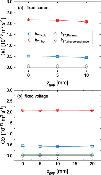
Figure 9. Ti ionization rate coefficients for different processes: ionization from collisions with electrons from the cold and the hot electron group ( and
and  ), Penning ionization from
  levels and charge exchange collisions with Ar+. Panel (a) shows results for discharges run in fixed current mode, panel (b) shows results from discharges run in fixed voltage mode. All rate coefficients are averaged over one pulse.
Download figure:
Standard image High-resolution image
Figure 10. (a) The probability of target species ionization αt as a function of  , and (b) the probability of target species ionization αt as a function of peak discharge current
  . The dashed line is a fit to the data points and results in the displayed equation. The best fits to the data points are given by the constants
  (A−1),
  (A−1) and
  (A−2).
Download figure:
Standard image High-resolution image
At first glance the results shown in figure 10(a) appear contradictory as a variation of one of the key discharge parameters, the magnetic field, has no influence on the probability of target species ionization αt in the fixed discharge current case. However, as discussed in section 3.1, an almost constant peak electron density  is a result of the constant peak discharge current. To test if
  (rather than the magnetic configuration) is the key parameter for αt, we plot αt as a function of
  , for the discharges run in fixed current and in fixed voltage mode (figure 10(b)). It gives a smooth curve that is steep at low discharge currents and levels off at high discharge currents.
The shape of the curve of αt vs.  can be understood by considering a Ti atom sputtered off the target and passing through the IR. The probability of an ionizing collision with an electron is then
where  is the average time it takes a sputtered atom to cross the IR and
  is the average time for ionization, and
  is the electron impact rate coefficient for ionization of the Ti atom. As the electron density varies during the pulse,
  varies with time during the pulse. The highest density of sputtered atoms is found at the time the current peaks [18]. Here we approximate
  . Assuming a constant crossing time, using equation (1), and summarizing all constant values (including
  that varies only little with
  , see figure 9) into a constant k1, we obtain (see appendix

A dashed line in figure 10(b) shows a fit of the data points to equation (11) with  (A−1). The fit in general reflects the trend of αt from which we conclude that the rising electron density from an increasing peak discharge current is the primary driver for the higher probability of ionization. However, we also note that the curve in figure 10(b) is slightly too steep and that a secondary effect is likely superimposed. We suggest that this secondary effect is gas rarefaction. At higher discharge currents, a higher degree of rarefaction can be expected which would decrease
  because, on average, sputtered atoms then experience fewer collisions within the IR. Assuming a linear variation of
  with
with  and summarizing again all the constants gives (see appendix

A fit of the data points to equation (12) is shown in figure 10(b) by a solid line. The fit shows an almost perfect match with the data points with the constants  (A−1) and
  (A−2). We therefore note that rarefaction is to be considered as a secondary effect to explain the shape of αt with
  . This has consequences as the increase in electron density and the increased degree of rarefaction with
  have opposing effects on αt. The gas rarefaction at high
  dampens the increase of αt.
Remember that the primary influence of αt is the variation of  caused by a varying
  . Due to the close link between
  and
and  , discussed in section 3.1, the probability of ionization αt can be well adjusted by varying the external process parameter
  . This was qualitatively already shown by Brenning et al [35].
4. Summary
We discuss the influence of the magnetic field on the electron density and electron temperature, which, in turn, determine the probability of target species ionization αt in a HiPIMS discharge. To quantify the effect of changes in the magnetic field strength and the degree of magnetic unbalance, we define an empirical magnetic field parameter that consists of summing the distances of the two magnet packs from the rear surface of the target. We denote this parameter  .
.
We find that the electron density closely follows the discharge current during the HiPIMS pulse, while the magnetic field only indirectly influences the electron density via the discharge current. On the other hand, the magnetic field has a large influence on the electron power absorption mechanism. The closer the magnets are to the target (smaller  ) the higher is the fraction of the total power that goes to electron energization, and the higher is the fraction of total electron energization that goes to Ohmic heating, i.e. electron energization in the potential drop across the IR. As a result, the cold electron temperatures are higher, and the hot electron temperatures are lower, when the magnets are close to the target.
Overall, however, the variation in the electron temperature remains too small to significantly influence the rate coefficients for target species ionization. This results in the probability of target species ionization being primarily dependent on the electron density, and thereby largely independent of the magnetic field strength. As the peak discharge current controls the electron density in the ionization region, it can be used to adjust the probability of target species ionization. At high peak discharge currents, the probability of ionization saturates at a level well below unity, which is an effect of gas rarefaction. With increasing degree of gas rarefaction at high peak discharge currents, the time for metal atoms to cross the IR becomes shorter due to fewer collisions with the rarefied argon working gas. This reduced residence time for sputtered metal atoms in the IR hampers electron impact collisions and results in a saturation of the probability of ionization with increasing peak discharge current.
Acknowledgments
This work was partially supported by the Free State of Saxony and the European Regional Development Fund (Grant No. 100336119), the Icelandic Research Fund (Grant No. 196141), the Swedish Research Council (Grant VR 2018-04139) and the Swedish Government Strategic Research Area in Materials Science on Functional Materials at Linköping University (Faculty Grant SFO-Mat-LiU No. 2009-00971).
Data availability statement
The data that support the findings of this study are available upon reasonable request from the authors.
Appendix A.: Ionizing collisions
In section 3.3 the probability of target species ionization is discussed and related to the discharge current. In the following, we will derive equations (11) and (12). Starting with equation (10) and using  from the discussion above, yields

Using now  where the numerical factor is from equation (1), yields

which is the sought equation (11).
Equation (12) can be derived in a similar manner. Using equation (A.1) and entering a linear variation of  with
with  , i.e.
  , where
  is the crossing time without any rarefaction and
  is a proportionality constant, yields
Summarizing again the constants into  and
and  yields equation (12).