

Abstract
The precision of magnet alignment in next-generation light sources is critical. To achieve this, the multipole magnets on a common girder of SPring-8-II, an upgrade of SPring-8, are planned to be aligned using the vibrating-wire technique. We developed an alignment monitoring system to monitor the magnet positions in the tunnel where the vibrating-wire technique cannot be executed while the magnets are not energized or when there are vacuum chambers in the magnet center. The alignment monitoring system utilizes a non-contact capacitive sensor embedded in a ceramic ball to measure the wire position relative to the center of the ball and derives the wire sag by measuring a higher mode eigenfrequency. The constitution of this system is illustrated for relevant studies, including the investigation of wire sag against the eigenfrequency, observation of the actual wire sag at a test bench, and validation of the system on the girders for the prototype magnets of SPring-8-II. The system measured the positions of a series of magnets with a precision of ±4 µm (peak to peak) in a 4 m range, in both the horizontal and vertical directions, meeting the requirement of SPring-8-II.
Export citation and abstract BibTeX RIS

Original content from this work may be used under the terms of the Creative Commons Attribution 4.0 license. Any further distribution of this work must maintain attribution to the author(s) and the title of the work, journal citation and DOI.
1. Introduction
Accelerator-based light sources have been successful tools for a wide variety of photon science and other applications. More than 30 facilities are in operation around the world. The storage ring of the light source, which produces synchrotron light, is built on a scale from several tens meters to several kilometers. The magnets of different types in the storage ring deliver the charged particle beam along a designated beam trajectory. To provide high brightness and stable lights to users, these magnets must be aligned with high accuracy to obtain a stable beam orbit. The requirement for the alignment precision is usually in the order of several tens of microns, depending on the particle dynamic design of each facility. A compilation of the alignment requirements for major facilities can be found in Leão et al [1]. To obtain low beam emittance the storage ring uses strong magnets. This makes the ring more sensitive to magnet misalignment. To reduce the sensitivity, the misalignment on a girder must be suppressed as much as possible [2]. For example, SPring-8-II, an upgrade of SPring-8, requires multipole magnets on a common girder (that holds a series of magnets in a straight section several meters in length) to be aligned within an error of 25 μm (standard deviation) [3], which cannot be achieved with the latest laser tracker or a laser CCD camera. A new instrument or method must be developed. The vibrating-wire method which measures the magnetic centers directly has been recently applied for this purpose [4, 5]. Nevertheless, this system cannot be executed while the magnets are not energized or when there are vacuum chambers in the magnet center. To keep the alignment precision, it is essential to develop a system that has comparable accuracy with the vibrating-wire system to monitor the positions of the fiducials (reference points for magnet alignment) of the magnets at a regular period.
In SPring-8, a laser technique was used to monitor magnet positions. In 1995, while installing the storage ring, we developed a laser CCD-camera system aligning the magnets on the common girder with a precision of 20 μm (σ) [6]. An iris diaphragm laser device was developed in 2014, with a measurement precision of approximately 10 μm (2σ) [7]. However, the laser system was not adopted for SPring-8-II because the magnet alignment utilizes the vibrating-wire technique, which requires the magnets to be energized during the alignment. A test of the laser beam stability affected by the heat flow was performed on a 4 m long marble table. In the experiment, a heating plate, heated 3 °C higher than room temperature, was placed below the measuring point (an iris target) to simulate an energized magnet, and the laser pointing stability was observed. The laser beam fluctuation grew by 50% on an average at each point. Consequently, the stability of the laser beam deteriorated by a factor of 1.5× √number of magnets. Concluding that laser is not the best choice in such an environment, a thermostable stretched wire system was investigated.
In the past, stretched wires have been used to align the components of accelerators [8–10]. Because the wire is not straight in the vertical direction due to gravitational sag, measurements are usually performed only in the horizontal plane, or the wire curve is calculated using a theoretical equation. Researchers at CERN have used a combined system of a wire position sensor (WPS) and hydrostatic level sensor (HLS) to determine the curve of the wire and realize two-dimensional measurements [11]. However, this method cannot be used in portable systems. Likewise, the two-axis optical sensors manufactured for the WPS [12–14] are not yet compact enough to measure the fiducials of the magnets.
We developed a magnet alignment monitoring system (MAMS) that utilizes a non-contact capacitive sensor embedded in a ceramic ball to measure the wire position relative to the center of the ball and derives the wire sag by measuring a higher mode eigenfrequency. This enabled us to monitor the magnet positions with a resolution of a few microns, even when the magnets are not energized or when there are vacuum chambers.
Generally, a system that uses a wire as a reference has to solve certain problems:
- (a)The curve of the wire is determined absolutely.
- (b)The factors affecting the wire position are corrected under real working conditions.
- (c)The wire position is correctly transferred outside in both transverse directions.
To solve problem (a), we calculated the wire sag using eigenfrequencies and determined the wire curve with sag. We demonstrated that a higher mode eigenfrequency has a higher resolution for wire sag. Additionally, we observed the actual wire sag at a test bench and compared it to the sag calculated by the eigenfrequency. For problem (b), we measured the wire eigenfrequency in situ, which removed the effect of the variations of linear density and tension in the wire while determining the wire sag under working conditions. Problem (c) was solved by transferring the wire position to the ball center, which defines a real point. We tested the measurement repeatability of the sensor along with the reproducibility of a set of sensors. We also validated this system on the common girders for the prototype magnets of SPring-8-II.
This alignment monitoring system was able to measure the positions of a series of magnets with a precision of a few microns, typically 4 μm in the 4 m range, in both the horizontal and vertical directions. It also allowed us to conduct a multi-target synchronous measurement.
2. Concept and constitution of the system
In this section, the constitution of the system is illustrated, and the theoretical forms calculating the wire sag from the eigenfrequency are summarized.
2.1. Constitution of the system
The MAMS, used to measure the relative positions of the fiducials of the magnets, is composed of a stretched wire, a series of sensor assemblies, and eigenfrequency measuring devices. Figure 1 is a schematic drawing showing the constitution of the system when setting up the prototype magnets of SPring-8-II. The instruments used in this system are listed in table 1. The fiducials were made on the top plates of the magnets. In addition to the fiducials, reference points for magnet pre-alignment using a laser tracker were made on the same plates.
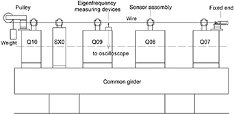
Figure 1. Constitution of the magnet alignment monitoring system (MAMS). It is mainly composed of a stretched wire, a series of sensor assemblies, and eigenfrequency measuring devices. It measures the relative positions of the fiducials of the magnets and monitors the variations.
Download figure:
Standard image High-resolution imageTable 1. Instrumentation of the magnet alignment monitoring system (MAMS).
| Instrument | Specification |
|---|---|
| Capacitive sensor | FOGALE WPS2D |
| Resolution | 0.1 μm |
| Range | ±5 mm |
| Ceramic ball | KYOCERA |
| Diameter | 3 in |
| Dimension error | 6 μm |
| Wire | NGK C1720W-EHM |
| Material | CuBe (0.2 mm) |
| Density (measured) | 2.629 × 10⁻⁴ kg m−1 |
| Laser displacement sensor | KEYENCE IL-S065 |
| Resolution | 2 μm |
| Oscilloscope | KEYSIGHT 3000 T |
The selected CuBe wire has good linearity with a diameter of 0.2 mm. It is heat-treated and naturally straight [5], stretched with a knife-edged pulley (Fogale Nanotech), which maintains constant tension.
The sensor assembly embeds a capacitive sensor [15] in a ceramic ball (KYOCERA). The two-axis sensor measures the distances between the wire and the electrode plate in two transverse directions. A schematic drawing of the sensor assembly is shown in figure 2 (only the electrodes on the y-axis are shown). The sensor's measuring center and the ball center are identical. Therefore, the sensor assembly measures the wire position relative to the center of the ball. Calibration and testing of the sensor assembly are illustrated in section 3.1. We used a ceramic ball because of its high dimensional precision and stability. Moreover, it separates the electrical field of the sensor from the metal base.
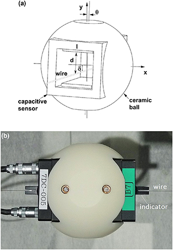
Figure 2. (a) Schematic drawing of the sensor assembly that measures the wire position relative to the ball center (only the electrodes of the y-axis are shown). The posture of the sensor is controlled by a round bubble level at the top to adjust the roll and pitch, and two indicators sticking to the sensor's two end surfaces over the wire at the symbol 'Ι' to adjust the yaw. (b) Top view of the sensor assembly.
Download figure:
Standard image High-resolution imageThe acquisition of the sensor measurement was performed with a digital multiplexer (Keithley 2701) through the LabVIEW interface. The output of the sensor was acquired continuously at a sampling rate of up to 1 Hz. Furthermore, all sensors on a girder were acquired synchronously. An example of the measurement is illustrated in section 3.4.
The eigenfrequency measuring device was used to measure the eigenfrequency of the wire to derive the maximum sag. It consisted of a laser displacement sensor and an oscilloscope. The spot size of the laser was chosen to be larger than the wire diameter. To measure the wire eigenfrequencies, we drew the middle of the wire up and released it to excite free vibrations. A method to excite the wire automatically involves employing a dipole magnet and introducing a pulsed current to the wire going through the magnet to excite the wire with Lorentz force. Although it is unnecessary for us in this work, this methodology enables a system to perform remote measurement. The amplitude of wire oscillation was measured by the laser displacement sensor at a sampling rate of 1 kHz, and performed the FFT process by the oscilloscope. Figure 3 shows a typical signal (color) of the oscillation amplitude for a 5.5 m long wire, the maximum amplitude was ∼2 mm, and the frequency component of the FFT in white. The peaks indicate the eigenfrequencies of each vibration mode. Because the resolution of the FFT is inversely proportional to the sampling time, a long sampling time leads to better frequency resolution. However, experiments showed that the damping time of a wire that is a few meters long was a few seconds, and higher-order modes attenuated sooner. Thus, we set the recording time to 10 s; consequently, the FFT resolution was approximately 0.05 Hz.

Figure 3. Measurement of the eigenfrequency. The color shows the signal of the oscillation amplitude for the 5.5 m long wire. White shows the frequency component of the FFT. The peaks indicate the eigenfrequencies of each vibration mode and are listed in the right column.
Download figure:
Standard image High-resolution imageTo examine the effect of nonlinear oscillation, concerning the magnitude of amplitude for instance, on the eigenfrequencies, a test was performed by dividing the collected data into two parts of 5 s each and performing Fourier transformation individually. The maximum difference of the eigenfrequencies between the first and second part was at the level of the frequency resolution (about 0.1 Hz for each case). The difference could be neglected and no effect of nonlinear oscillation was observed. Therefore, we processed the data of 10 s as a whole.
2.2. Wire sag and curve
We calculated the maximum wire sag using eigenfrequencies and determined the wire cure with sag.
The curve of the hanging chain follows a catenary. If the lowest point is defined as the origin, the equation of a catenary has the form [16]
Taking the quadratic approximation of cosh (x/a) at the origin, equation (1) can be expressed by the parabola

The chain stretched with a tension of T (N) has [17]

where ρ is the linear density (kg m−1 ) of the wire and g is the gravity acceleration. The curve of the wire is then described as
Let the length of the wire be L, the sag in the middle of the wire is thus expressed in terms of ρ and T as
In the frequency domain, a uniform wire with two fixed ends vibrates in standing waves with discrete eigenfrequencies [18]:
where  is the number of vibration modes.
Substituting equation (4) in equation (3), the maximum sag of the wire is derived in terms of the eigenfrequency as
For n = 1 [4],
where  is the eigenfrequency of n-order (Hz); that is, the maximum sag of the wire depends only on the eigenfrequency.
The maximum sag can be deduced from the eigenfrequency of any vibration mode. However, utilizing a higher mode eigenfrequency leads to a higher sag resolution. By differentiating the sag with respect to  in equation (5), the resolution of the sag is given by that of the frequency as follows:
That is, the resolution of the sag derived from the n-order eigenfrequency is n-times higher than the fundamental frequency. Moreover, the resolution of the sag is inversely correlated with the cube of the fundamental frequency. As the length of the wire increases, the resolution of the wire sag remarkably decreases because of the low natural frequency. Hence, it is important to use higher mode eigenfrequencies.
Substituting equation (3) in equation (2) and shifting y by the amount of the maximum sag, the curve of the wire is in the form of
Note that the sag here represents the displacement of the wire from a straight line connecting its two endpoints. Even if the two endpoints have different heights, equation (8) is still applicable, as illustrated in appendix
3. Experimental details and results
In this section, the measurement accuracy of the sensor assembly is examined. The experiment of the relative change of wire sag correlated to the eigenfrequency and the investigation of absolute wire sag against the eigenfrequency measurement are demonstrated. Additionally, the validation of the system on the common girder for the prototype magnets of SPring-8-II is illustrated.
3.1. Measurement accuracy of the sensor assembly
3.1.1. Measurement repeatability of the sensor assembly.
The capacitive sensor measured the distances between the wire and four electrode plates (figure 2). It had a measurement range of ±5 mm and a high linearity region of ±1 mm at the central zone. The output voltage was directly proportional to the distance (Vout= kd, ±5 V). The center of the sensor was defined at 0 V. The offset of the center from the rotating center was calibrated by measuring the displacements of the wire from the 0 V point at two opposite positions in the direction of the roll. The central offset was obtained by averaging the displacements. The measuring center was thus the sensor's center compensated with the central offset.
The sensor is structurally symmetric to its center. The random tilt of the sensor does not affect the output if the wire passes through the ball center. Otherwise, it introduces a measuring error that approximately equals the product of the wire offset and the sensor's rotation angle (δ × θ). In most cases of short-range magnet alignment, the amount of wire sag is below 1 mm. The corresponding measuring error is within 1 μm if the random tilt of the sensor is less than 1 mrad. To control the tilt, we set the posture of the sensor assembly using a round bubble level (precision: 0.3 mrad) at the top to adjust the roll and pitch, and two indicators (figure 2(b)) to adjust the yaw by rotating the sensor and visually fitting the slits of indicators to the wire, making the sensor plates parallel to the wire. We confirmed the repeatability of the measurement of the sensor assembly at various wire offsets. We first performed five repetitive measurements with the wire at the ball center, resetting the sensor assembly at each measurement and shifting the wire in the vertical direction by 0.25 mm at each step. Figure 4 shows the measurement uncertainty in the x-axis against the wire offset in the y-direction; it is 0.5 μm in a standard deviation at a 1 mm offset. In addition, the uncertainty is small, approximately 0.2 μm, when the wire offset is below 0.5 mm, because it is comparable to the measuring noise of the sensor. Likewise, the wire offset in the x-direction brings measurement uncertainty in the y-axis.

Figure 4. Measurement uncertainty of the sensor assembly in the x-direction against wire offset in the y-direction, the sensor assembly was reset at each measurement. The wire was shifted in the y-direction by 0.25 mm at each step. Dashed line: linear function fitting.
Download figure:
Standard image High-resolution image3.1.2. Reproducibility of the sensor assembly.
To measure the positions of a series of magnets on a common girder, it is crucial for a set of sensors (four to seven according to the number of magnets) to be mutually exchangeable and have an identical scale factor and central position. To calibrate the scale factor, we set the sensors on a calibration table at the same time and shifted the wire at the sensor's central zone with the standard linear gauges (Mitutoyo LGF-0110L). To ensure the identity of the central positions, we set up three points in a straight line at equal intervals, as shown in figure 5. We mounted each sensor on the middle point in turn and measured its displacement from the straight line connecting the centers of two reference sensors on both sides ( ). The displacements among the sensors were compared. The same wire was used in the calibration, and the two reference sensors were kept stationary. Thus, the measurement error was the repeatability of the sensor assembly. The displacements of the central positions from the nominal ball center in the x–y plane for a set of sensors are shown in figure 6. After compensating for the dimensional difference of the balls inspected by the manufacturer, we confirmed that the reproducibility of the central position for the sensors was within ±2 μm (maximum).
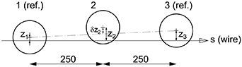
Figure 5. Top view of the layout of central position confirmation. Each sensor was mounted on the middle point in turn and the displacement from the straight line connecting the centers of two reference sensors was measured.
Download figure:
Standard image High-resolution image
Figure 6. Displacements of the central positions from the nominal ball center in the x–y plane for a set of sensors. Open circle: without dimensional correction. Closed circle: after compensating for the difference in diameters of the balls.
Download figure:
Standard image High-resolution image3.2. Validation of the eigenfrequency measurement
We investigated the changes in the wire sag related to the eigenfrequency (equation (6)). To validate whether the system is sensitive to a minute change in sag, the standard Kevlar carbon wire for alignment (Fogale Ltd, ρ= 3.22 × 10⁻⁴ kg m−1, 0.5 mm diameter) was used, considering it causes small sag because of high tension. Using the layout in figure 1, the 2.2 m long wire was initially stretched with a tension of 6 kg, corresponding to a fundamental frequency of approximately 100 Hz. We increased the tension by adding a nut of ∼15 g to the weight at each step and measured the change in the fundamental frequency. Each step corresponded to a 0.07 μm sag change. Figure 7 shows the sags derived from the frequency for each step and the positional movements of the wire measured by the sensor assembly; the two movements were consistent with each other at a sub-micron level. Moreover, the changes in the eigenfrequency (not shown) due to the increments of the tension exactly followed equation (4). Because the variation of the sag was small at each step, the wire position was measured at every second step (0.14 μm) and was averaged 50 times.

Figure 7. Changes in wire sag relating to the eigenfrequency as the tension increased. Open square (left axis): the sag derived from the eigenfrequency for each step. Open circle (right axis): the positional movements of the wire measured by the sensor assembly.
Download figure:
Standard image High-resolution imageAs mentioned in section 2.2, a higher mode eigenfrequency has a high resolution for wire sag. Moreover, as the length of the wire increases, the resolution of the wire sag decreases. When the sag resolution by the fundamental mode is below the required value, it is important to use higher mode frequencies. This was experimentally demonstrated in appendix
3.3. Comparison between the absolute sag and the eigenfrequency measurement
To investigate the distribution of the wire sag, we used the same test bench described in Fukami et al [5], and compared the actual sag against the sag obtained from the eigenfrequency measurement.
Figure 8 shows a schematic drawing of the test bench. A WPS was mounted on a carriage and the height of the wire with respect to the carriage was measured. The carriage moved on a guide rail with a straightness of ±0.02 mm and 4 m in length. The height of the carriage was measured by a pair of HLS, with a movable HLS setting on the carriage connected to a fixed one beside the guide rail. The HLS provided an absolute height reference of the geoid for sag measurement. In addition, two electrical levels (WYLER AG) were mounted on the carriage to compensate for the errors of the roll and pitch. A ∼5.5 m long CuBe wire was stretched above the guide rail with a tension of 2 kg between the two endpoints at equal elevation. The parameters of the instrumentation are listed in table 2.

Figure 8. Schematic drawing of the test bench for the wire sag measurement. Upper part: Side view of the bench. A wire position sensor (WPS) and a hydrostatic level sensor (HLS) were set on the carriage to measure the height of the wire relative to a fixed HLS (not shown). Lower part: Top view of the carriage. Two electrical levels were used to correct the errors of the roll and pitch of the carriage.
Download figure:
Standard image High-resolution imageTable 2. Parameters of the instrumentation.
| Instrument | Specification |
|---|---|
| WPS sensor | OGALE WPS1D |
| Resolution | 0.1 μm |
| Range | ±1.25 mm |
| HLS sensor | FOGALE HLS-STD |
| Resolution | 0.1 μm |
| Range | 2.5 mm |
| Electric level | WYLER |
| Sensitivity | 1 μrad |
| Range | ±20 mrad |
Therefore, the height of the wire with respect to the hydrostatic surface of the fixed HLS was measured as

In the measurement, the carriage moved in steps of 100 mm each and waited for 30 s until the water in the HLS reached equilibrium. It took 30 min for one measurement of the 4 m rail. A typical distribution of the wire sag is shown in figure 9, with s = 0 at the first point of measurement. The wire positions were fitted with equation (8) by the least-squares algorithm and extrapolated to two endpoints. The deviation of wire positions from the parabola was 0.6 μm in a standard deviation, which we believe is due to the linearity of the wire.
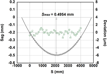
Figure 9. Typical distribution of the wire sag measured at the test bench. Open circle (left axis): sags at the measuring points at an interval of 100 mm. Solid line: parabola fitted to the measuring points with equation (8). Smax indicates the maximum sag in the middle of the wire. Open square (right axis): deviations of the measuring points from the parabola.
Download figure:
Standard image High-resolution imageThe repeatability of the sag measurement was tested by repeating the above measurement ten times in three consecutive days. It was 0.5 μm (σ), as shown in figure 10. The mean sag was observed at 0.4953 mm. The temperature of the guide rail was monitored using thermocouples at six points in 80 cm intervals. It fluctuated by approximately 0.8 °C during the experiment. This caused a sag change ( ) of approximately 0.01 μm when considering the linear density change owing to wire expansion. Thus, the temperature did not affect the sag measurements.

Figure 10. Repeatability of the sag measurement. The measurements were performed ten times in three consecutive days.
Download figure:
Standard image High-resolution imageIn contrast, the eigenfrequency was measured, and the maximum sag was calculated using the 5th-order eigenfrequency. We did not use higher modes than the 5th order because the deviations of the eigenfrequencies were increasing. This was considered to have happened because of the relatively small oscillation amplitude which leads to a worse SN ratio. In addtion, higher modes attenuate sooner; thus, the FFT resolution decreases. As illustrated in the Discussion section, we adopted an eigenfrequency of more than 100 Hz, which provides enough accuracy to calculate the sag. The measured 5th-order eigenfrequency was 124.440 Hz on an average, which is in contrast to the theoretical frequency (equation (4)) of 124.446 Hz. The corresponding sag was 0.4944 mm with a resolution of 0.4 μm. It differs from the wire sag measurement by −0.9 μm.
In addition, we compared the actual sag to the eigenfrequency measurement for 2.5 kg tension at the test bench. The results are listed in table 3. In this table, the titanium wire (Goodfellow) was tested on a common girder of the magnets, because they are often used in the magnetic measurement of multipole magnets [19].
Table 3. Comparison of the sags obtained from different methods.
| Wire | Sag_f (mm) | Sag_m (mm) | Sag_t (mm) | δS (μm) |
|---|---|---|---|---|
| CuBe 1 a | 0.4944 | 0.4953 | 0.4944 | −0.9 |
| CuBe 2 b | 0.3952 | 0.3964 | 0.3958 | −1.2 |
| Ti-Al c | 0.0811 | 0.0809 |
Note: Sag_f: the sag obtained from eigenfrequency measurement; Sag_m: sag measured at the test bench; Sag_t: theoretical sag from equation (3). a φ0.2 mm, ρ= 2.629 × 10⁻⁴ kg m−1, L= 5.4906 m, T= 2.004 kgf. b φ0.2 mm, ρ= 2.629 × 10⁻⁴ kg m−1, L= 5.4906 m, T= 2.503 kgf. c φ0.2 mm, ρ= 1.369 × 10⁻⁴ kg m−1. L= 3.767 m, T= 3.0 kgf.The values of ρ and T were measured with a precise balance and a tension meter (Tokyo Sokki TCLZ-50NA).
The difference between the sag derived from the eigenfrequency and that of the real measurement (δs in the table) was approximately 1 μm. It is sufficiently small and acceptable when considering the following reasons restricting the accuracy of real measurement: (a) the measuring range was comparatively short for the wire length due to the spatial restriction, and (b) the straightness error of the wire was observed to be in the range of ±1–2 μm and was periodic along the length [5].
3.4. Measurement on the common girder of magnets
The MAMS was validated on the common girders for the prototype magnets of SPring-8-II. The wire was fixed on the two end magnets, and the sensor assemblies were mounted on the magnet fiducials. The system could be set up in 30 min and completed measurement in 10 min. It is a portable system and is suitable for periodical observations of magnet positions in the tunnel. Each sensor was compensated for the central offset, scale factor, and sag in the vertical plane. The output of the sensor was measured with a moving average for one minute and a standard deviation of approximately 0.1 μm. Figure 11(a) shows an example of the measurement of the magnet positions in the vertical direction, as shown in figure 1. The periodic variations of the magnet positions were due to the fluctuations of cooling water and room temperature. The transverse relative positions of the inner points relative to the two ends were calculated at every moment. The measurement repeatability of the MAMS was evaluated on the same girder by replacing the wire and resetting the sensors four times. The deviations of magnet positions from the first measurement are shown in figure 11(b). The maximum deviations were ±3 μm and ±2 μm for the horizontal and the vertical directions, respectively. The errors included the measurement uncertainty of the sensor assembly, the linearity error of the wire, and the measurement error of the sag.

Figure 11. (a) Example of the measurement in the girder as shown in figure 1, showing the variations of magnet positions in the vertical direction. (b) Measurement repeatability of the MAMS when the sensors and the wire were reset or replaced four times.
Download figure:
Standard image High-resolution imageWe constructed a test half-cell lattice of SPring-8-II. The multipole magnets on the girder were aligned using a vibrating-wire alignment system [5]. This system utilizes a wire excited with an AC passing through the magnets and detects the center of the magnetic field by scanning the vibrating amplitude of the wire at its resonant frequency. The total random error for the magnet alignment was tested at 1.7 μm (σ). Thereafter, the MAMS was used to record and monitor the positions of the magnets. We considered performing the magnet alignment of SPring-8-II on the common girder at an assembly area and then transport it to the tunnel. To simulate the transportation and confirm the alignment status, we used a truck and transported the precisely aligned girders as a whole from an experiment hall to an assembly building. The changes in relative positions of the magnet before and after transportation were measured using the two systems. The results for the girder in figure 1 are listed in table 4. It was demonstrated that the magnet positions monitored by the MAMS agreed with those measured by the vibrating-wire system for a maximum of 6 μm, which is within the maximum deviation (±6.4 μm) between the two systems by individual error estimation.
Table 4. Changes of magnet relative positions after transportation.
| Magnet | VW system (x,y) μm | MAMS (x,y) μm |
|---|---|---|
| Q8 | (+8, −3) | (+11, +2) |
| Q9 | (+7, +4) | (+8, +7) |
| SX0 | (−3, −3) | (+3, +3) |
4. Discussion
The advantage of our approach in deriving the wire sag by measuring the higher mode eigenfrequency is discussed here.
The curve of the fine wire is described by the catenary and can be approximated from the parabola. The key parameter of the parabola, the sag maximum, can be calculated using the theoretical equation or the natural frequency.
To calculate the sag using the theoretical equation, one needs to know three parameters: linear density ρ, tension T, and length l. Using equation (3), the relative error of the sag can be derived as
Therefore, to ensure 0.1% precision (1 μm for a 1 mm sag) of sag, the error for ρ, T, or l alone should be no more than 0.1% or 0.05%. Because the laser tracker has a distance precision better than 1 ppm, the error for the third term can be neglected. The precise tension meter (strain gauge) also meets the requirement while measuring the horizontal force of the wire directly. However, to determine the linear density precisely, one should know the exact wire length at the tension exerted because the CuBe wire extends 0.2% for the material we used. One should also ascertain that there is no variation for different manufacturing lots. Moreover, for a synthetic material (Kevlar), the density was reported to be affected by humidity. Thus, it is essential to know the actual density of the wire under working conditions.
In contrast, to determine the sag using higher mode eigenfrequency, the density or other parameters of the wire are not required. According to equations (4)–(7), the relative error of sag is derived as

That is, assuming that the resolution of frequency ( ) is not related to the vibration mode, the relative error of sag is less than 0.1% if one selects a higher mode eigenfrequency that is more than 100 Hz. This is easily achieved with a short-range wire or by increasing the wire tension. In addition, if the sag resolution is sufficiently high, one expects a long measuring range. Based on equations (4) and (7) for the wire we used (ρ= 2.629 × 10⁻⁴ kg m−1,
  ), the wire length depends on the number of modes and sag resolution by
where  is the sag resolution. Assuming that a system is required to have a sag resolution of 1 μm, the wire length should not be longer than 4.36 m if
  . In contrast with the fundamental mode, the 6th-order mode expects the measuring length to be extended to approximately 8 m theoretically, with almost the same sag resolution.
Thus, determining the sag using higher mode eigenfrequency has a better resolution compared to the theoretical equation and could extend the measuring range.
5. Conclusion
We developed an alignment monitoring system that measures the positions of the fiducials of the magnets on the common girder. The system utilizes a non-contact capacitive sensor embedded in a ceramic ball to measure the wire position relative to the center of the ball. It transfers the wire position to a real point precisely. We measured the wire eigenfrequency using a simple method of exciting free vibrations. Therefore, it is possible to obtain the wire sag in situ without knowing the values of linear density and tension of the wire. We calculated the wire sag using a higher mode eigenfrequency, demonstrating a higher resolution for the sag. We validated our approach by investigating the distribution of the wire sag at a test bench. The difference between the actual sag and the sag obtained from the eigenfrequency was small. The measurement uncertainty of the sensor assembly was approximately 0.2 μm when the wire offset from the center was below 0.5 mm. The measurement reproducibility for a set of sensors was within ±2 μm (maximum). The resolution of the wire sag was 0.4 μm at the test bench. Thus, the system can measure magnet positions in a range of several meters with a precision of ±4 μm (peak to peak), providing the CuBe wire with good linearity. Although the effect of environmental factors such as airflow or vibration on wire position is not considered, this alignment monitoring system meets the requirement of SPring-8-II and will be first used in the 3 GeV light source project.
Acknowledgments
We would like to thank C Mitsuda at The High Energy Accelerator Research Organization (KEK) and K Kajimoto at SPring-8 Service Co. Ltd for collaborating with us in testing this system using the magnetic field measurement device. This work was supported by the RIKEN SPring-8 Center (RSC). The authors are grateful to H Tanaka and T Ishikawa for supporting us throughout the development of this system.
Appendix A.: Definition of the sag
Sag is defined as the displacement of the wire from the straight line connecting two endpoints (figure A1). Here, equation (8) holds true even if the two endpoints have different heights.
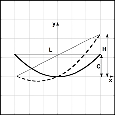
Figure A1. Solid line: The catenary with two endpoints in level. Dash line: The catenary with two endpoints having a height difference.
Download figure:
Standard image High-resolution imageThe catenary with two endpoints in level has the form
The sag, displacement from the reference line  , is given as
However, the catenary with two endpoints having a height difference of H can be expressed as [20]
where  and L is the wire length.
Substituting the first two terms of the power series for the cosh functions, it can be approximated as
Therefore, the displacement from the reference line  is
is
It is the same form as the sag obtained by the catenary of two endpoints in level.
Appendix B.: Sag resolution of higher mode frequency
From equation (7), the resolution of the wire sag is inversely correlated to the cube of the fundamental frequency. Therefore, as the length of the wire increases, the resolution of the wire sag remarkably decreases because of the low natural frequency. When the sag resolution by the fundamental mode is beyond the required value, it is necessary to use higher mode frequencies. As demonstrated below, a higher mode frequency is more sensitive to the sag change.
In this experiment, a Kevlar carbon wire (ρ= 3.22 × 10⁻⁴ kg m−1, 0.5 mm diameter) was used since it is commonly utilized in long-distance alignment because of its low linear density [11, 14]. It is flexible and has a similar character to the chain used in the definition of equation (1). Initially, the 33 m long wire was stretched with a tension of 10 kg. The fundamental frequency was 8.4 Hz and the sag resolution was estimated to be 50 μm. We increased the tension by 10 g-force at a step, corresponding to a 4 μm sag change, and measured the eigenfrequencies. This process was repeated ten times. Figure B1(a) shows the variations in the eigenfrequency for each vibration mode from the beginning as the tension increased. Because the change in the fundamental frequency was under the FFT resolution, ten measurements overlap as two points in the figure. The differences between the sag derived from the eigenfrequencies and the sag calculated using the theoretical equation (4) are shown in figure B1(b). It is demonstrated that the sag resolution (3σ deviations) of the 6th-order mode (6.8 μm) is higher than that of the fundamental mode (46.1 μm).

Figure B1. (a) The variations of the eigenfrequency from the beginning for each vibration mode as the tension is increased by 10 g-force at a step. Symbol + indicates the theoretical frequencies from equation (4). (b) Differences between the sag derived from the eigenfrequencies and the sag calculated by the theoretical frequencies.
Download figure:
Standard image High-resolution image