

Abstract
The resonance characteristics of vibrating structures change when they are immersed in fluids and these changes can be related to the parameters density and viscosity of Newtonian liquids. The various suitable structures, vibration modes, transduction principles, and signal analysis methods lead to an immense variety of sensor systems reported in the literature. In this review, we focus on the basic similarities between various electromechanical transducers and their evaluation methods and show that despite the apparent differences, a common design route can be followed. It is outlined that single vibration modes can be approximated by damped harmonic oscillators where the hydrodynamic loading is accounted for by a general model. The two common classes of sensors, the piezoelectric and the electrodynamic, can be described by dual circuits such that the same resonance estimation method can be applied. Also, the limitations associated with this unified approach are discussed. Furthermore, aspects concerning interface circuits and accuracy-limiting factors, such as noise and interference, are reviewed.
Export citation and abstract BibTeX RIS

Original content from this work may be used under the terms of the Creative Commons Attribution 4.0 license. Any further distribution of this work must maintain attribution to the author(s) and the title of the work, journal citation and DOI.
1. Introduction
Resonant sensor principles can be used for measuring a variety of technically relevant parameters. In this review, we discuss vibrating electromechanical structures for sensing liquid viscosity and density as well as associated recent developments and unifying approaches.
The principle of using resonant sensors, where the measurands influence the resonance characteristics, is appealing because a vast number of measurands can be measured somehow using a resonant sensor as outlined is in the book of Elwenspoek et al [1]. The advantages of this approach include higher immunity of frequency signals to noise compared to amplitude signals and a higher dynamic range. Furthermore, accurate measurement of frequencies is comparatively simple, due to widely available and cheap reference oscillators. However, [1] emphasizes also that these advantages do not necessarily include high accuracy, good repeatability, and low hysteresis. These and other limitations, which also apply to fluid sensors, are reviewed in this work in more detail.
The article is structured as follows. In section 1, general features of resonant fluid sensors are discussed including relations between electrical and mechanical equivalent circuit representations, as well as single degree-of-freedom approximations of the resonance characteristics by damped harmonic oscillators (DHOs). Section 2 covers various piezoelectric and electromagnetic fluid sensors and their associated equivalent circuit representations. A general model for the viscous drag forces acting on vibrating bodies is presented in section 3. Aspects of resonance parameter extraction from spectral data are discussed in section 4. Aspects concerning the electrical excitation and read-out interfaces are discussed in section 5. In section 6, noise sources, related to thermal fluctuations, as well as, interferences are reported.
1.1. Proximity sensor: a simple example of a resonant sensor
Before fluid sensing is discussed, an intuitive example, which reveals the general limitations of resonant sensors, is shown. A very basic representation of a resonant sensor is an inductive proximity sensor where the inductance of the coil of an LC oscillator is increased by an approaching iron body causing a reduced oscillation frequency. Feeding the output of a frequency counter into a look-up table yields the proximity to the iron part. The picture changes if the distance to non-ferromagnetic metal objects shall be detected. The induced eddy currents in a nearby piece of aluminum, for instance, slightly reduce the effective inductance but the finite conductivity of the metal introduces losses causing a reduced oscillation amplitude. The amplitude signal is more sensitive in this case, requiring a different kind of readout electronics, e.g. an envelope detector and a threshold switch. This introductory example already shows the dilemma of resonant sensors. Typically, each circuit measures one of the two fundamental characteristics of a resonance, either the resonance frequency fr or the vibration amplitude which is closely linked to the quality factor Q (also termed Q-factor). Even if a more sophisticated circuit determined both quantities, the involved unknowns namely the distance, the permeability, and the conductivity cannot be determined unambiguously from fr and Q, causing at least one fundamental cross-sensitivity. Secondary cross-sensitivities, such as the temperature influence on circuits and geometry, long-term drifts of components, etc are rendered tolerable by design but impede the accuracy. As will be shown in more detail later, neglected cross-sensitivities can be the dominant accuracy limiting factor.
1.2. Representations of electromechanical transducers
A transducer can be defined as a device that transforms energy from one domain (i.e. electrical, mechanical, chemical, thermal, magnetic, or optical) to another [2]. Engineers concerned with problems with different energy domains, often depict the whole problem in a domain familiar to them. Fluid sensors are mostly electromechanical transducers that can be conveniently represented by electrical equivalent circuits. The book of Lenk et al [3], for instance, presents a comprehensive treatment of equivalent circuit representations of electromechanical transducers and how to derive them. For the lumped-element mass-spring-damper system, a fully equivalent simple RLC circuit consisting of resistor  , inductor
  , and capacitor
  as shown in figure 1 can be found. Both systems are referred to as DHOs, or in case of no damping (
 ) as simple harmonic oscillators (SHOs). Equivalent electrical transmission line models can be used to represent distributed vibrating structures which feature a discrete spectrum of natural frequencies, i.e. a fundamental mode and its overtones. Finding exact expressions that describe a resonant sensor is only possible for a very limited number of cases, such as for the one-dimensional approximation of a piezoelectric disk sensor. However, direct use of these equations is impractical in most cases anyway. The equations of spatially distributed resonating structures such as quartz disk sensors include acoustic transmission line equations which disguise the resonance characteristics (i.e. the poles of the transfer functions) in meromorphic functions, which are hard to interpret by inspection of the equation. However, if a pole expansion [4] of the transfer function is determined, the series of resonances is revealed. Equivalent circuit representations can then be found, e.g. by using the Brune network synthesis method [5]. For instance, Martin [6] shows the process for the fluid-loaded quartz crystal microbalances (QCMs). However, for more complex structures such as the fluid-loaded tuning fork, no closed-form representation can be found. But, if it is assumed that such a function and an approximating pole expansion can be obtained, it is evident that the equivalent circuit could be represented by a series of DHO elements for the harmonic modes and additional components. For the piezoelectric disk sensor discussed in section 2.1.3, the static capacitance C0 in the Butterworth–Van Dyke model is such an additional component. When only the resonance characteristics are of interest, these components are considered spurious, e.g. in [7, 8], or parasitic [9].
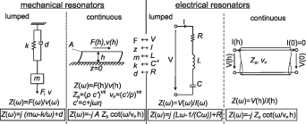
Figure 1. Equivalence of electrical and mechanical impedances of basic resonators.
Download figure:
Standard image High-resolution image2. Sensor technologies
Figure 2 shows some examples of resonant sensor structures. The cantilevers, bridges, tuning forks, and diaphragms typically vibrate in flexural modes which can be excited by piezoelectric, electromagnetic, or thermal means, or by Brownian motion of the surrounding fluid. Surface acoustic wave (SAW) sensors use piezoelectric transduction but electromagnetically excited SAWs were reported also, e.g. in [10]. As for most sensor technologies, also resonant fluid sensing is a field where many disciplines intersect. For instance, the constitutive equations provided by the theories of elasticity and rheology are required to describe the resonator material and the fluid to be measured. Electrodynamics, continuum mechanics, and fluid dynamics are used to establish the governing equations which are solved by mathematical tools providing a relationship between electrical and mechanical quantities. The electrical signals are usually transferred to the digital domain using readout electronic circuits, where they are evaluated using digital signal processing. Designing an accurate fluid sensor, therefore, requires detailed knowledge of each aspect of the measurement problem. An overview of a wide range of sensor technologies for viscosity and density sensing including piezoelectric, electrodynamic, and micromachined sensors is provided in the review [11]. In the following, technologies are categorized into the two main groups piezoelectric and electrodynamic sensors, due to the different mechanical impedances associated with these transducers (i.e. piezoelectric and electrodynamic sensors correspond to high force to low displacement and low force to high displacements, respectively). Coupling to the fluid impedance requires therefore adequate sensor structures. The literature relevant for fluid sensing is extensive, and therefore for each discussed technology that follows, a review on the relevant available reviews and books is presented first as suggested starting points for further reading.

Figure 2. Elastic structures used for fluid sensing.
Download figure:
Standard image High-resolution image2.1. Piezoelectric sensors
Transduction principles based on the piezoelectric and the inverse piezoelectric effects [12] are exploited for many resonant sensor applications using a variety of sensor geometries. E.g., in Pang et al [13] piezoelectric sensors for chemical and biological applications in liquid environments are reviewed. They cover extensional and shear-mode piezoelectric sensors (film bulk acoustic resonators (FBARs) and QCM) as well flexural (cantilevers and membranes) sensors.
2.1.1. Piezoelectric disk sensors.
Instead of LC circuits, piezoelectric quartz crystal disks are often used as frequency-determining elements in electronic circuits, due to their high frequency stability, low production tolerances, and costs. For the thin platelets, the thickness modes are the dominant modes of vibration including the two shear modes and the extensional mode. Typically, the thickness-shear mode (TSM) as shown in figure 3 is preferred for a quartz oscillator. When the housing of such an element is removed and the faces are exposed to the environment, these elements represent versatile sensors for a variety of physical properties. Therefore, the field of fluid sensing draws heavily from the findings of resonator research for frequency control such that many resonators originally designed as timebases were directly used in sensing. Although the design of these resonators seems to be guided solely by the requirements of frequency control, EerNisse [14] in his early review identified cross-fertilization with the sensor field, where findings in sensor research contributed to the high sophistication of quartz timebases. Various quartz bulk acoustic wave (BAW) sensors for different physical properties including temperature, forces, thin-film mass and stress, gas density and pressure are surveyed in [14]. The structures are differentiated by their modes of vibration (thickness-shear, single-ended flexural, double-ended flexural, and torsional) and although only quartz is considered in this work, most of the effects apply to other sensor materials with many being even more pronounced when metals instead of crystals are used. For instance, in [14] is discussed that certain orientations of the crystal cut result in zero temperature dependence of the resonance frequency which reduces cross-sensitivity to temperature. This is particularly beneficial for accurate fluid density measurements because the inertial fluid forces associated with the fluid mass influence mainly the resonance frequency of the resonator. First sensing applications of TSM resonators included mass sensing and these sensors were therefore termed quartz crystal microbalances (QCMs). The frequency change due to a thin mass layer attached allover the sensor surface follows the well-known Sauerbrey equation [15]. Immersed in viscous fluids, a frequency change proportional to the square root of the viscosity (η) times density (ρ) is observed, as derived by Kanazawa and Gordon [16]. Pioneering research in this field can also be attributed to Martin et al [6, 17]. Since then, QCM sensors have matured and books on applications in biology and chemistry [18], soft matter research [19], and thin film and surface science [20] are available. While piezoelectricity is treated theoretically in many books, e.g. [12, 21–30], only a few mention fluid interactions [31–33]. Applications of QCM sensors for oil viscosity sensing in automotive and industrial environments are reported in [34–36]. An optimized QCM design for harsh environments is reported in [37].

Figure 3. (a) Piezoelectric slab with thickness field excitation (TFE) of a shear mode. (b) Realization of a resonator disk with top and bottom metalization as used in electronic circuits.
Download figure:
Standard image High-resolution imageQCMs are attractive sensor elements but they feature spatial sensing constraints. The vibration amplitude profile (vx ) for a thickness-shear sensor in contact with the liquid is shown in figure 4. The evanescent acoustic velocity field in the liquid decays exponentially with the characteristic decay length δ given by
Decay lengths are typically low (e.g. 250 nm at 5 MHz in water), such that, e.g. in emulsions, only one phase may be sensed [38]. Similar issues occur with other, more complex fluids. Flexural vibrators such as tuning forks and cantilevers described in the next paragraph can conveniently be realized for low frequencies, thus avoiding potential issues concerning fluid heterogeneity.
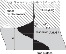
Figure 4. Velocity profile in the TSM resonator for a one-sided fluid loading. The shear displacement profile decays exponentially in the fluid.
Download figure:
Standard image High-resolution image2.1.2. Quartz tuning forks and cantilevers.
Auerbach [40] in 1878 was the first to realize that the pitch-change of a tuning fork immersed in liquid depends on viscosity and density. In EerNisse [14], next to TSM resonators, also single and double ended flexural mode resonators are considered which include the now prominent quartz tuning forks (QTFs) and microcantilever sensors. The QTF originally designed for timekeeping (shown in figure 5) features a resonance frequency of 32.768 kHz (i.e. 215 Hz). The fundamental mode of vibration shown in the figure can be considered as that of two cantilevers connected to a common base. Compared to a single cantilever beam, the bending moments of both cantilevers compensate, such that support losses (also known as anchor [41], attachment [42], or mounting [43] losses) are reduced. As shown, e.g. in [41], the support losses are not limited to the vicinity of the mounting point but can interact in a complicated manner with the whole structure. For fluid sensors, this can imply that the mounting condition (e.g. the mounting torque of a screw-mount sensor) can detune the sensor in a non-predictable way. It is therefore advisable to reduce mounting losses by resonator design, if possible. QTFs are well suited for measuring viscosity and density. As will be discussed in section 3 in more detail, the fluid displacement profile features shear wave and potential flow components. Fluid density and viscosity act on the resonator in such a way that viscosity and density can simultaneously be determined from the resonance characteristics as is reported, e.g. in [39, 44–52]. QTFs are also applicable at extreme conditions including millikelvin temperatures for liquid helium sensing [53] under high hydraulic pressures [39] and in down-holes for oil recovery [54–56]. In addition to the application for liquid measurement, numerous quantities can be measured with the help of tuning forks. These include gas density as reported, e.g. in [57–60], biomolecule binding to functionalized surfaces [61, 62], gas moisture sensing [63–65], and force sensing [66–68]. In his review [69], EerNisse also mentions the measurement of temperature, pressure, and acceleration. The tuning fork also experienced great popularity as an alternative to cantilevers for atomic force microscopy (AFM) [70–75] and quartz enhanced photoacoustic spectroscopy [76, 77].
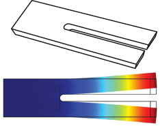
Figure 5. Quartz tuning fork and fundamental mode of vibration. The typical oscillation frequency of the 6 mm long commercial tuning forks is 32.768 kHz (see, e.g. [39]) Reproduced from [39]. CC BY 4.0.
Download figure:
Standard image High-resolution imageWhile the free fundamental angular vibration frequency ω0 of the typically thin rectangular cantilevers (length L, density ρ, cross-sectional area A and bending stiffness EI, as shown in figure 6) is well described by the Euler beam theory as [78]
the effect of viscous fluid loading acting on them is mathematically difficult, and closed-form equations are only available for special cross-sections. Theoretical treatments of the viscous drag forces acting on cantilevers are discussed in [79–83]. Viscosity and density sensing is reported in [84–97]. Alternative applications for cantilevers are manifold including for instance, chemical [98–102], biological [103, 104] and photoelectric [105, 106] sensing. The review on microelectromechanical systems (MEMS) cantilevers for mass and fluid sensing by Mouro et al [97] goes into detail about mathematical modeling of the elastic cantilever, showing the various mode-shapes and DHO approximations of the single modes. The fluid loading on the vibrating beam is represented by the dimensionless hydrodynamic function (see, e.g. [79, 107]), which is reviewed in more detail in section 3. Lange et al [108] extensively cover the design and fabrication of CMOS cantilevers for AFM and gas sensing in their book. Zhao et al [109] review coupled MEMS sensors which feature largely increased sensitives for sensing mass (see also [110, 111]). Applications in viscous environments are shown in [112] for laterally coupled QCMs and in [113, 114] for self-excited coupled cantilevers.
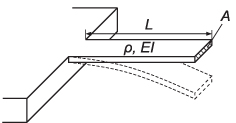
Figure 6. Cantilever vibrating in the fundamental mode.
Download figure:
Standard image High-resolution image2.1.3. Equivalent circuits for piezoelectric sensors.
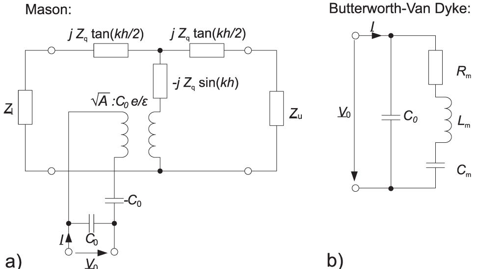
The Mason model [26, 117] in figure 7(a), or the Redwood or KLM equivalent circuits [24, 118], for instance, can be used to describe the thickness modes of a quartz disk sensor. As is further shown in [24], the transmission line models can be approximated by various lumped-element representations, where each mode of vibration is accounted for by a respective LC circuit. The most famous lumped-element representation is known as the Butterworth–Van Dyke (BVD) model [26] shown in figure 7(b), where series LC circuits (i.e. the motional arms) for each harmonic mode are connected in parallel to a static capacitance. While the  and
and  values can be derived from geometry and material parameters, the material losses are difficult to predict and are mostly accounted for by an additional series resistor
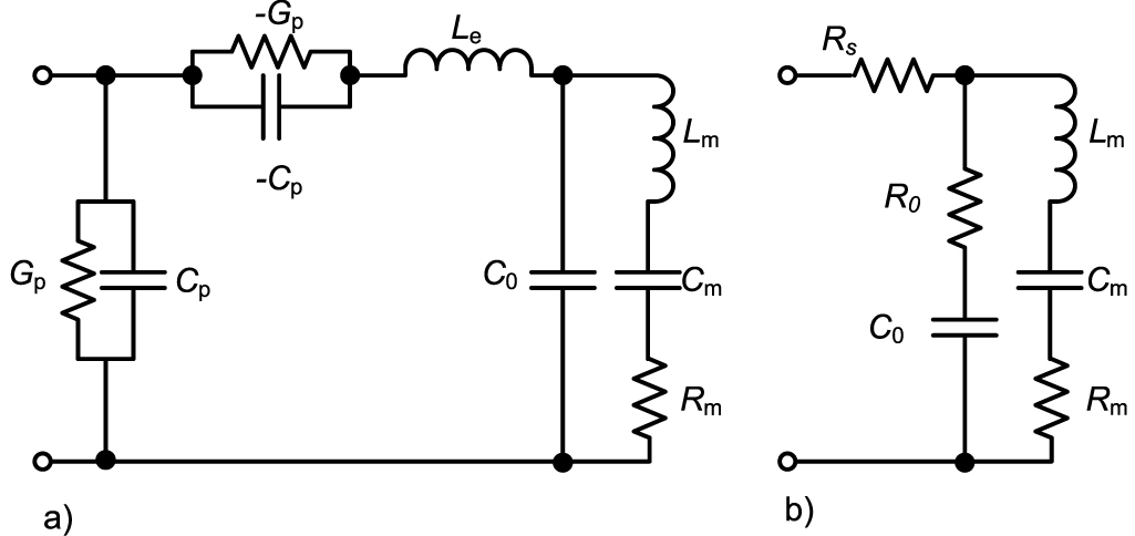
  which is determined using vacuum measurements. In the extensive overview of Ballato [115], the derivations of the single models and a historical overview of equivalent circuit representations are provided for piezoelectric but also for piezomagnetic and bimorph structures. Ballato et al [119] point out that material losses are often added in an unjustified manner and propose modifications for the BVD, shown in figure 8(a), for piezoceramics, which naturally feature higher losses and higher piezoelectric coupling factors than, e.g. quartz or refractory oxides. They take into account acoustic viscosity (AV), DC conductivity, piezoelectric and piezoelectric losses, which cause complex coupling factors and wavenumbers requiring modifications of the BVD for plate resonators. When using the standard BVD model, it must therefore be kept in mind, that particularly for higher losses and coupling factors an adaption may be necessary. For piezoceramic material characterization see, e.g. [121–123]. A more realistic consideration of bulk loss mechanisms for thin FBARs is the mBVD model proposed in [120, 124] (shown in figure 8(b)), where a resistor
  is added in series to the BVD circuit with an extra resistor R0 in series to the static capacitance C0. The thus modeled structures considered in [120] featured a resonance frequency of 1.9 GHz. The two additional components were adjusted for best agreement with network analyzer measurements.

Figure 7. Mason and Butterworth–Van Dyke (BVD) equivalent circuits. The fluid loading on upper and lower side of the piezoelectric disk is modeled by respective impedances  and
and  in the Mason model. The trigonometric functions are required to model the transmission line characteristics which include all higher harmonics. The BVD model shows one motional unloaded branch. Overtones are implemented by additional series RLC in parallel (see, e.g. [115, 116]).
Download figure:
Standard image High-resolution image
Figure 8. Extended BVD models with more realistic representations of losses. (a) The model from [119] includes DC conductivity and dielectric loss of the piezoelectric material by Gp and Cp . The mass of the electrodes is considered by Le and AV by Rm . (b) The mBVD model from [120] for FBAR sensors uses two additional elements for better agreement with measurement results at high frequencies.
Download figure:
Standard image High-resolution imageThe fluid acting on a vibrating structure introduces an additional mass drag and viscous losses. These influences are represented in the BVD model by an additional inductance  (mass drag) and a series resistor
  (viscous losses), as shown in figure 9. Additional electrical loss mechanisms are considered by the effective electrical fluid admittance
  , if both electrodes are in contact with the fluid or the electric fields penetrate the fluid, e.g. through a thin insulation layer. The resonance parameters of the fluid-loaded sensor are that of the extended motional branch. The influences of the static capacitance and the electrical fluid loading are considered spurious to the DHO behavior of the motional branch. The model is adequate for representing QCM [6, 116], piezoelectric cantilevers [125, 126], and QTF sensors [47, 48] but also applies to more complex sensors. In [127] a glass plate and piezoelectric ceramic composite vibrating at a higher antisymmetric Lamb mode, in [128] an aluminum nitride-based resonator using the so-called roof-tile mode, and in [129] a CMUT fluid sensor were all successfully modeled by the BVD.
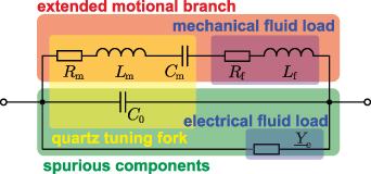
Figure 9. Viscous fluid loading adds mass ( ) and viscous loss (
 ) components to the BVD [39]. The electrical fluid load
  has to be considered in case of fluid shunting the electrodes. Reproduced from [39]. CC BY 4.0.
Download figure:
Standard image High-resolution imageThe EBVD model for thickness shear mode sensors vibrating in viscoelastic fluids is shown in figure 10(b) [131]. It is based on the so-called LEM in figure 10(a) [130], where the mechanical fluid loading is described by a complex-valued impedance. For viscoelastic fluids characterized by a complex shear modulus  , [131] shows that the equivalent fluid impedance can be modeled by a series RLC instead of an LR circuit.

Figure 10. (a) Lumped-element model (LEM) [130] and (b) extended Butterworth–Van Dyke model (EBVD) [131] taking into account viscoelasticity by  .
.
Download figure:
Standard image High-resolution image2.2. Electrodynamic transducers
Apart from various piezoelectric sensors, in his review [132], Langdon shows various types of fluid sensors which use electrodynamic transduction principles, such as fluid-filled vibrating pipes excited by electromagnets and read-out inductively by an additional coil or by the excitation coil itself. As the fluid in the vibrating pipes adds mass to the structure proportional to fluid density and the fluid is not significantly sheared, these sensors are accurate density sensors with low cross-sensitivity to viscosity. The same transduction principle is used for a fluid density sensor consisting of a thin-walled fluid-filled cylinder actuated to a circumferential wave mode. Also, an oscillating sphere sensor for measuring dynamic viscosity is discussed. It vibrates at low frequencies such that the force acting on the sphere can be approximated by the Stokes force [133]. Figure 11 shows various setups using electrodynamic transduction principles: (a) shows a double U-shaped sensor from [134] featuring a density-sensitive fluid-filled and a viscosity-sensitive solid wire vibrating in a fluid, (b) is a spiral spring fluid sensor [135], (c) is a steel tuning fork [136] vibrating in a fluid, (d) from [137] and (e) from [138] show dominant shear vibrating platelet sensors. Research related to vibrating platelet sensors is also reported in [137–144]. (f) Shows a silicon platelet excited to various modes from [145] used for contactless sensing of fluid properties and mass loadings. Similar setups using steel platelets are discussed in [146, 147]. (g) from [148] and (h) from [149] show torsional resonators for sensing the viscosity-density-product also known as the AV [150–152]. An updated structure adding density-sensitive fluid chambers to (g) was reported recently in [153], which allows simultaneous measurement of density and viscosity.
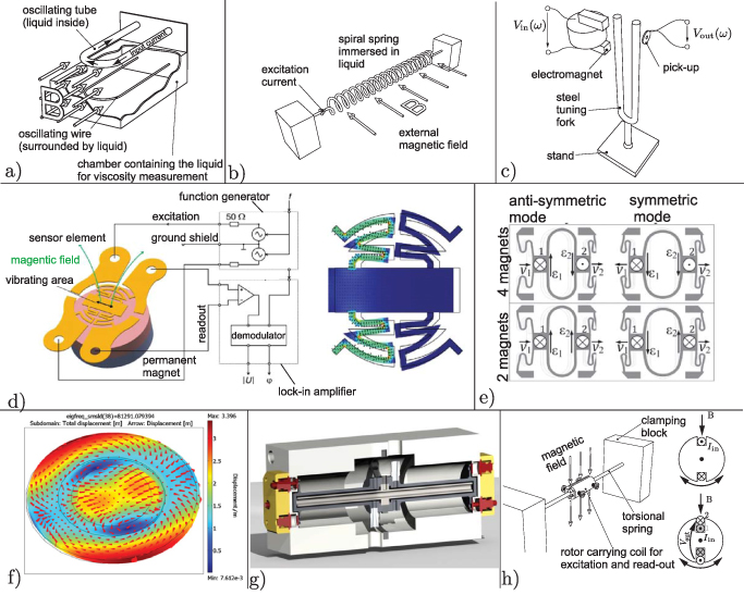
Figure 11. Examples for electrodynamic transducers from the author's research group [134–138, 145, 148, 149]. (a) Reprinted from [134], Copyright (2013), with permission from Elsevier. (b) Reprinted from [135], Copyright (2014), with permission from Elsevier. (c) Reprinted from [136], Copyright (2015), with permission from Elsevier. (d) Reprinted from [137], Copyright (2009), with permission from Elsevier. (e) Reprinted from [138], Copyright (2015), with permission from Elsevier. (f) © 2006 IEEE. Reprinted, with permission, from [145]. (g) Adapted from [148]. CC BY 4.0. (h) Reprinted from [149], Copyright (2015), with permission from Elsevier.
Download figure:
Standard image High-resolution image2.2.1. Equivalent circuits for electrodynamic sensors.
The shown electrodynamic sensors use Lorentz-force excitation and voltages generated by motion induction as readout signals. Figure 12 shows three representatives of such structures from [154]. For the vibrating sensor in (a), an electrically insulating platelet is attached to two mutually insulated pre-stressed wires. A time-harmonic current  (underlined quantities are complex-valued with the imaginary unit
  ) in one of the wires in combination with a perpendicular static magnetic field B produces a time-harmonic force per length
  causing a vibration of the wires of length l and the platelet. At a particular resonance, the resonant structure can be represented by a spring-mass-damper system with respective effective mass
  , stiffness
  , and damping
  . The effective vibration velocity in the frequency domain is
with c denoting a mode-shape factor. The induced voltage  in the second wire, forming the readout signal is therefore
The Bode and the Nyquist plots shown on the right of figure 12 resemble that of a DHO with no visible cross-talk. For the wire sensor in (b), one wire is used for simultaneous excitation and readout. Therefore, the small induced voltage is superimposed on the driving voltage across the wire of resistance R0, resulting in an ohmic cross-talk

This causes a shift of the Nyquist plot on the real axis. The double diaphragm sensor (c), originally devised by [155] and further investigated in [156–162] uses two elastic polymer diaphragms, each carrying conductive paths for readout and excitation. Therefore, the cross-talk due to ohmic effects are excluded, however spurious coupling occurs due to inductive cross-talk caused by voltage induction between excitation and readout-path of each diaphragm but also between the two diaphragms. This kind of cross-talk causes a superimposed straight line to the spectra of the DHO. The induced voltage including the coupling inductance L0 and a wire resistance is

The value of the coupling inductance L0 for a given diaphragm layout is a function of the distance of both diaphragms, the mode-shape and if both diaphragms vibrate in the same (density sensitive mode) or the opposite (viscosity sensitive) direction [160]. As is pointed out in [163] a small coupling inductance  nH for the two-wire sensor (a) could be identified in the measured spectra and attributed to the mutual induction between both contacting wire loops. To reduce this effect, and more importantly, to stabilize it, the areas were reduced to a minimum and the contact wires were fixed, as is shown in figure 13.

Figure 12. Three electrodynamic viscosity sensors described by Heinisch et al [154]. (a) The two-port suspended platelet sensor shows a DHO characteristic. (b) For the one-port vibrating wire setup, a comparatively large ohmic cross-talk is apparent. (c) The inductive cross-talk caused by the coupling inductance of excitation and readout path distorts the Nyquist plot of the DHO to a balloon-like shape. Reproduced with permission from [154].
Download figure:
Standard image High-resolution image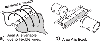
Figure 13. Influence of wiring on inductive cross-talk [163]. Keeping areas A small reduces cross-talk. For fixed wiring, the coupling inductance can be estimated and compensated by signal processing. Reprinted by permission from Springer Nature Customer Service Centre GmbH: Springer. [163] © 2011.
Download figure:
Standard image High-resolution image2.3. Other MEMS sensors
This paragraph is devoted to micromachined sensors excluding the previously mentioned tuning forks and microcantilevers. The variety of such micromachined fluid sensors is immense, and topical overviews are given by Abdolvand et al [164], by Mishra [165] and in the thesis of Bilic [166] who provide comprehensive overviews on modeling, fabrication and application of micromachined (MEMS) resonators. They cover modeling of single resonances by equivalent DHOs, equivalent circuit representations, various structures and their mode shapes, intrinsic damping mechanisms and anchor losses, transduction principles (capacitive, piezoelectric, thermal/piezoresistive). Furthermore, details on process flows for fabrication of capacitive transducers, piezoelectric layers, CMOS MEMS, and packaging are provided. Interface electronics and performance issues for applications including timing, oscillators, and RF-filters are reported, but also sensing of mass depositions, changes of elastic stiffness, and pressure. Many aspects discussed in these publications are relevant for fluid sensing. Concerning fluid sensing, Stemme and Enoksson [167, 168] report on various structures including vibrating beams, bridges, diaphragms, torsional twist, comb drives, and spiral spring-supported platelets. A recent review focusing on automotive applications including fluid sensing is given by Mohankumar et al [169].
In contrast to piezoelectric TSM resonators, where the acoustic standing wave is distributed over the whole thickness, in SAW devices the acoustic wave is guided along a surface and the acoustic energy is concentrated there. TSM resonators are therefore often referred to as BAW devices. Most often the term SAW is used as a synonym for Rayleigh waves, i.e. an elastic wave propagating along the surface of an elastic half-space where the motion of the vibrating particles features surface normal and longitudinal components, yet no shear component. Using piezoelectric substrates or layers in combination with the deposition of so-called interdigital transducers can serve to excite SAWs. An interdigital transducer represents an insulated but interlaced pair of electrodes, which upon application of an AC voltage generate a periodic electric field pattern matching the periodicity of the desired wave. The fact that the acoustic energy is concentrated at the surface makes these devices even more sensitive than TSM resonators to, e.g. mass loading at the surface. The SAWs can be used in delay line or resonator devices. However, when loaded with a liquid, the surface normal components of the displacement lead to generation of pressure waves in the liquid causing significant damping of the wave, which is why Rayleigh waves are not used for liquid sensing applications. Thus, wavemodes featuring shear polarized vibration are preferred for sensing in liquids. Since (at least isotropic) half-spaces do not support surface-guided elastic shear waves, the surface can, e.g. be structured with a grating (surface transverse waves) [170] or provided with a waveguiding overlayer (Love waves) [171]. Further related devices are so-called shear-horizontal plate modes or flexural modes in thin membranes (Lamb waves), which, even though the feature surface normal displacements, do not radiate acoustic pressure waves into a liquid if the associated (typically low) phase velocity is below the speed of sound in the liquid. [31] and [172] provide an overview on many of these modes and [173] reviews the application of BAW and SAW in automotive applications (including sensing of liquid media). Approaches for wireless communication with passive SAW sensors are reviewed by Pohl in [174]. Although fluid sensing is not mentioned, the reported applicability in harsh environments may be exploited for robust fluid sensors. While SAWs and related modes can be used as resonator sensors (and many of the concepts reviewed here apply), they are very often used in a delay line setup, which is why we leave the reader with this superficial overview on SAW sensors and refer to specialized literature for further details.
3. Forces on oscillating bodies in fluids
Using dimensional analysis (see, e.g. [175]) shows that the complex-valued fluid drag force  acting on a vibrating structure can be written as

For time-harmonic excitation, the Ansatz  , with the complex force amplitude
  , the real part Re(·), and the angular frequency ω. (Note, that also the conjugated form is often used in literature, i.e.
  .) The fluid force is determined by fluid density ρf, a characteristic volume V and the dimensionless so-called hydrodynamic function
  .
.  is a complex-valued function (
 ) of the dimensionless number
  and all aspect ratios αi
which define the shape of the structure. L and δ represent the dominant sensor dimension and the characteristic decay length of plane shear-waves
and all aspect ratios αi
which define the shape of the structure. L and δ represent the dominant sensor dimension and the characteristic decay length of plane shear-waves  (see (1)), respectively.
  is directly related to the non-dimensional frequency β in Tuck [107], which is also termed Reynold's number in the works of Sader's group [79, 176, 177].
3.1. Oscillating sphere
This introductory example features a transversely oscillating sphere in liquid attached to a lossy spring. The driving force for the fluid-loaded mass (m) spring (k) damper (d) system is

Introducing the eigenfrequency  and the vacuum quality factor
  yields for the fluid-loaded resonance parameters ωr
and Qr
:
yields for the fluid-loaded resonance parameters ωr
and Qr
:
This simple form is obtained when the volume V in (7) equals the volume of the vibrating mass of density ρs
, i.e.,  . According to [133] the real and imaginary parts of the hydrodynamic function for the sphere are
The two resonance parameters in (9) are functions of the unknown fluid density ρf and viscosity η, only. In the limit  and using
  , the fluid force in (7) reduces to the Stokes law
  .
.
3.2. Vibrating beams
It is shown, e.g. in [80, 92], that for distributed resonators, such as vibrating cantilevers, bridges and tuning forks, etc similar relations apply. E.g., for cantilevers with circular cross-section, a set of effective spring, mass, and damping parameters can be determined for each mode of vibration (see, e.g. [97]). For prismatic cantilevers, the hydrodynamic function for the fluid force per length is used
The closed-form expression for  and the commonly used truncated power series representation for its real and imaginary parts are
K0 and K1 in (12) denote modified Bessel functions of the second kind. This approach, however, neglects flow along the elongated dimension of the cantilever and around the cantilever tip. The computation of  is generally difficult and closed-form expressions are available only for a limited number of problems including vibrating spheres [133], infinitely long cylinders [178], and blades [107]. For beams of square and rectangular shape, no closed-form solutions for
  are known, but numerical methods are utilized, e.g. in [177] and [83].
3.3. Dominant shear sensors
Vibrating disk or platelet sensors are used to measure the viscosity-density product but they are limited when it comes to measuring the individual parameters. When an area element A of an infinite plate is considered (i.e. edge effects are neglected), the hydrodynamic force acting on the faces is given by [178]

This already reveals that the product  appears, which can not be separated. The force equation can be brought into a form compatible with the approach described above
This, however, requires the introduction of an artificial length L to define a characteristic volume for surfaces. The real and imaginary parts of the hydrodynamic function turn out to be identical in this particular case
This equality is a consequence of pure shear motion and makes the measurement of individual densities and viscosities impossible. This relation is for instance also obtained for the fluid-loaded QCM where L corresponds to the thickness of the piezoelectric disk. To show this, resonance frequency and Q-factor expressions for series RLC circuits using the equivalent electrical components of the BVD circuit (e.g. from in [6] or [179]) are substituted into (9). Transforming the equation yields  . The pre-factor k is approximately 1 and depends on the electromechanical coupling constant of the piezoelectric material.
3.4. Rotating and torsional structures
For rotating or torsional sensors, the balance of torques is considered. The fluid-induced torque is again a function of  [148, 149, 180–183]. The hydrodynamic function for torsional blades is reported, e.g. in [184].
3.5. Limitations of the approach
The fluid flow of linear viscous media is described by the Navier–Stokes equations (NSEs) [185]
By comparing the quantities in the NSE, it is apparent, that the effects of second viscosity parameter λ related to viscous losses in compressional deformation and pressure gradients  connected to fluid compressibility, were neglected in the hydrodynamic functions discussed above. For a purely compressional wave, the longitudinal viscosity
  is relevant, but its effect is mostly concealed due to the low compressibility of liquids. It is therefore not required to consider λ for sensing shear viscosity and density. Setups designed to determine λ are shown, e.g. in [186–189]. Finite compressibility of fluids is conveniently described by a finite speed of sound c. Van Eysden [82, 176] derived a hydrodynamic function considering compressible fluids by introducing an additional dimensionless number
  . The fluid force acting on flexural vibrating structures is mostly approximated by the force per length of an infinitely extended rigid body, which, according to [82, 184], is an over-simplification in situations where the mode numbers are high and significant displacements in the long dimension occur. Furthermore, the predicted onset of efficient pressure wave radiation is affected by this simplification [190]. To account for the mode-shape, [176] uses a dimensionless wavenumber κ for the elongated dimension. The fluid force in (7) depends linearly on the velocity but the convective part in the NSE
  is non-linear which gives rise to various fluid instabilities [191] when vibrational amplitudes are comparatively large. Reynold's numbers are defined for each instability together with a critical value that must not be exceeded. These critical numbers can be determined by perturbation methods, as is shown, e.g. in [192, 193] where the stability of the flat Stokes layer is considered. This type of instability is particularly relevant for vibrating fluid sensors and occurs at the interface of the fluid and a plane shearing surface, where velocity gradient and therefore the convective part is largest. The definition of Reynold's number, according to [193], is given by
  with the critical value being around 708. Therefore, the shear displacement amplitudes should be much smaller than 708δ, which is most often satisfied for piezoelectric sensors such as thickness shear mode quartz resonators with maximum displacement amplitudes of 10–200 nm in vacuum and gases [194] and even more so in fluids. For cantilevers vibrating in fluids, Sader [79] concludes that any length scale of the beam must largely exceed the vibration amplitudes (X). For compressional waves, Beigelbeck [195] remarks that velocity amplitudes have to be small compared to the occurring wavelength of pressure waves. Strictly, the hydrodynamic function
  depends therefore on a larger set of dimensionless numbers, e.g.
  . To be able to determine ρf and η from ωr
and Qr
, the spurious effects have to be rendered negligible by design. The DHO approximation poses an additional limitation for distributed structures with many modes of vibration, such as QCMs and QTFs. To be able to consider one resonant mode alone by a DHO equivalent, it is required that nearby modes do not noticeably interfere with the mode under consideration, which is not guaranteed, e.g. when low-Q resonances in highly viscous fluids occur. The resonant frequencies of unwanted cantilever modes can be adjusted by placing additional mass [196], attaching absorbers [197], or tailoring the width over length [198], for instance. The NSE describes Newtonian i.e. linear viscous fluids, only, but all real fluids are non-Newtonian at least to some extent. Many substances including, e.g. biofluids [199], polymers [200], and polyelectrolytes [201] are characterized by complex stress to strain relations. These complex fluids are extraordinarily diverse with a wide variety of available models [199, 202–204] which however present no complete description for all possible fluid deformations.
. To be able to determine ρf and η from ωr
and Qr
, the spurious effects have to be rendered negligible by design. The DHO approximation poses an additional limitation for distributed structures with many modes of vibration, such as QCMs and QTFs. To be able to consider one resonant mode alone by a DHO equivalent, it is required that nearby modes do not noticeably interfere with the mode under consideration, which is not guaranteed, e.g. when low-Q resonances in highly viscous fluids occur. The resonant frequencies of unwanted cantilever modes can be adjusted by placing additional mass [196], attaching absorbers [197], or tailoring the width over length [198], for instance. The NSE describes Newtonian i.e. linear viscous fluids, only, but all real fluids are non-Newtonian at least to some extent. Many substances including, e.g. biofluids [199], polymers [200], and polyelectrolytes [201] are characterized by complex stress to strain relations. These complex fluids are extraordinarily diverse with a wide variety of available models [199, 202–204] which however present no complete description for all possible fluid deformations.
4. Resonance estimation
The term resonance estimation in this context means the determination of the resonance parameters of the motional branch described in section 2 from sampled spectral data. For the sensors discussed here, such spectral data will, in general, be given in terms of impedance (admittance) spectra. Accurate determination of resonance frequency and Q-factor are mandatory to retrieve accurate density and viscosity values. Viscous damping acting on vibrating fluid sensors reduces the Q-factor (e.g. to 6.1 for a QTF in a fluid with ρf = 834.1 kg m−3 and η = 242.9 mPa s [175]) which impairs the accuracy of the determined resonance parameters. Higher dampings cause broader resonance characteristics and lower amplitudes, such that in the presence of noise, the frequency peak is not as clearly localized as for high-Q resonances. Furthermore, the signal amplitude is reduced, causing a reduced signal-to-noise ratio. Both effects translate to standard deviations σρ
and ση
of estimated density and viscosity featuring approximate proportionalities of  and
and  for the QTF [175]. Accurate determination of resonance parameters in order to give accurate viscosity and density readings is therefore more demanding in higher viscous fluids. Various approaches for resonance estimation are reported in the microwave literature [205–215] which prepared the ground for precise resonant fluid sensors. Among the available methods, only the ones using complex frequency spectra are considered here ignoring methods using only magnitude signals such as reported in [216, 217]. Petersan and Anlage [207] compare different resonance estimation methods with regard to accuracy when cross-talk, phase shifts, and moderate noise are present. Although they consider the spectra of scattering parameters of microwave cavities, the reviewed methods also apply to complex immittance signals (i.e admittance and impedance signals). The methods are based on a lumped-element approximation of the resonating structure. For instance, the motion-induced voltage expression in (4) is equivalent to a parallel RLC circuit. Inductive cross-talk and wire inductance and wire resistance add a series inductor L0 and a series resistor R0 to the equivalent circuit. Using the respective definitions for series and parallel RLC quality factors, it can be shown (see, e.g. [218]) that the circuit representations of piezoelectric sensors featuring an electrical fluid load and the electrodynamic sensors with series components caused by cross-talk or wire resistance and inductance are represented by the dual circuits in figure 14. Group delay of cables, and phase errors or phase changes in the readout circuit due to calibration errors, thermal effects, or aging are accounted for by a phase shift in figure 14. The determination of the individual L, R, and C parameters of the lumped-element equivalent circuit form complex immittance signals represents an ill-posed problem. Estimating the
  and Q, e.g. from the admittance
  of a typical motional branch
by direct optimization using, e.g. Gauss-Newton iteration [219] fails in presence of noise, due to the bad numerical condition. A simplification commonly used is to assume  , yielding the Lorentzian approximation
for which robust estimation is discussed in [207]. It is shown in [207] that using inverse mapping methods based on circle-fits of the Nyquist plots are robust against spurious components that cause translation and phase shifts φ of the Nyquist plot. The fitted circle-center  includes shifts due to frequency-independent spurious components, such as the ohmic cross-talk for the wire sensor in figure 12(b). By subtracting the circle-center from the Nyquist plot and calculating the phase function
it is shown that robust estimation of the parameters Q,  , and φ is possible. Regrettably, the method is only efficient for high-Q resonances but produces intolerable deviations for fluid sensing applications with Q mostly smaller than 100 [220]. Furthermore, the cross-talk in piezoelectric and electrodynamic sensors feature frequency-dependent components which not only shift the Nyquist plot but also distort it. Estimating also frequency-depending cross-talk in microwave signals is shown, e.g. in [208, 221, 222] where extended geometrical-algebraic approaches based on circle fitting are used. Niedermayer et al [220] carry the idea of the inverse mapping method further by employing a decomposition of the frequency response in motional branch and background signals. The spurious background signal is approximated by a broadband frequency-dependent function of second order and subtracted from the measured immittance, leaving the motional branch, from which the phase is determined as mentioned above, but without using the Lorentzian approximation. Figure 15 from [223] shows the effectiveness of the background subtraction approach for a QCM disk fully immersed in water while a minute amount of salt (NaCl) dissolves over a period of 15 min. While the added salt does not change viscosity and density noticeably, the changing salinity causes distortions of the 90 sampled resonances due to the changing spurious background signal. The right figure shows the 90 motional branch admittances
  after background subtraction. The method is immune to the electrical and electrochemical processes influencing the recorded spectral data. The level of distortion of Nyquist plots encountered in fluid sensing using QTFs is even more pronounced as shown in figure 16 [39], where no circles are apparent at higher viscosity but which can be retrieved using the background subtraction method of [220].
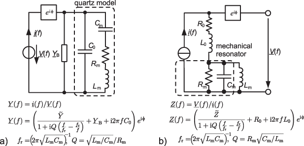
Figure 14. Equivalent circuits for piezoelectric (a) and electrodynamic sensors (b). The duality of the circuits allows using the same resonance estimation method for electrodynamic and piezoelectric sensors as is described in detail in [218]. © 2015 IEEE. Reprinted, with permission, from [218].
Download figure:
Standard image High-resolution image
Figure 15. (a) Admittance of the QCM while salt dissolves for 90 recorded spectra over 15 min. (b) The motional branch admittances for the 90 resonances draw on top of each other [224]. Reprinted from [224], Copyright (2012), with permission from Elsevier.
Download figure:
Standard image High-resolution image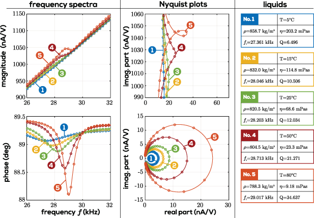
Figure 16. In the left two plots, the frequency responses of measured and fitted admittance signals of a QTF immersed in silicone oil at various temperature set-points ranging from 5 ∘C to 80 ∘C are shown. Only small phase shifts indicate resonances. The magnitude plot is dominated by the linear slope caused by C0. The associated Nyquist plot is shown in the above middle figure. The background signals were subtracted, leaving only the motional branch admittances, which resemble circles shown in the lower middle figure. The solid lines represent fitted results using a resonance estimation algorithm, and the markers show measured data points. On the right, the liquids corresponding to the labels (1–5) and the measured resonance parameters are listed [39]. Reproduced from [39]. CC BY 4.0.
Download figure:
Standard image High-resolution image5. Electrical interfaces
General commercial instruments commonly used for the read-out and driving of fluid sensors include lock-in amplifiers, impedance analyzers, and network analyzers. Modern impedance analyzers, such as the E4990A from Keysight, use the auto-balancing-bridge measurement technology and are accurate (e.g. a typical basic accuracy of  in measured impedance) with a large dynamic range (e.g. from 10 mΩ to 100 MΩ). The frequency ranges from 20 Hz to 120 MHz. Vector network analyzers (VNAs) targeted for radio frequency measurements, determine the scattering parameters referenced to a system impedance of typically
  . For two-port analyzers, the impedance matrix
  relating input and output voltages to the associated currents
 ![$[ \underline{U}_1, \underline{U}_2]^T = \underline{\boldsymbol{Z}}~\cdot~[ \underline{I}_1, \underline{I}_2]^T$](https://content.cld.iop.org/journals/0957-0233/33/1/012001/revision2/mstac2c4aieqn67.gif) can be calculated from the matrix of scattering parameters
can be calculated from the matrix of scattering parameters  by [225]

with
I
denoting the identity matrix. For sensor impedances far-off Z0, as is often the case for fluid sensors, the reflection coefficients  and
and  at both ports are close to one. Accuracies of calculated impedances from scattering parameters therefore typically lag behind that of dedicated impedance analyzers. Nevertheless, VNAs are regularly used for the evaluation of resonant fluid sensors, as shown, e.g. in [226–229].
However, the majority of dedicated systems are not miniaturizations of the aforementioned universal analyzers, but rather tailored closely to the specific sensor type using alternative methods of sensor evaluation targeting at reduced costs and size. These include for instance harmonic oscillators [9], ring-down (decay) measurements [230, 231], as well as reactance- and phase-locked-loop (RLL, PLL) circuits [232–234].
5.1. Interfaces for piezoelectric sensors
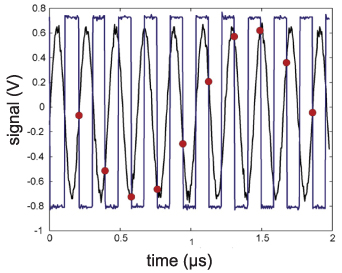
The benefits and drawbacks of using commercial impedance and network analyzers for interfacing AT-cut quartz disks are discussed in the review by Arnau [9]. He concludes that the benefits include that (i) the device can be measured in isolation with no external circuitry influencing the measurement, (ii) parasitic influences can be excluded by calibration, and (iii) differentiated information in relation to diverse contributions of the load can be obtained. On the downside, he mentions (iv) cost and dimensions (v) sometimes an inconvenient connection between equipment and sensor and (vi) limited capability for multiple sensor evaluation. In the recent review by Park and Choi [235], the list is updated and newer references are included. Both contributions emphasize analogous interfaces with electronic compensation of parasitics and attention to heavy fluid loads. Arnau reviews analog oscillator circuits including emitter-coupled, active, and balanced bridge types. Circuits with one quartz electrode grounded are considered better suited for QCM under liquid loading. He points out that transistor-based oscillator circuits, in general, suffer from temperature-dependent parameters, parasitic capacitances, and non-linearities. A remedy is presented in form of operational transconductance amplifiers, also known as diamond transistors. The control signal of an automatic gain control (AGC) circuit implemented to maintain a stable oscillation amplitude can be used as a damping indicator in addition to the resonance frequency. A chapter devoted to AGC is found, e.g. in [235]. PLL circuits with parallel capacitance compensation using linear integrated circuits are discussed as well. Particularly, the static capacitance compensation in PLL circuits is crucial for PLLs [236]. So-called dual-mode oscillators as described Vig [237] excite and track two harmonic resonances intended to increase the gathered information. As is outlined in [237], e.g. the spurious temperature changes can be separated from the wanted mass change information in micro-balancing applications. An analog circuit using a dual PLL principle is reported in [179] and is intended to track fundamental mode and an overtone. It is furthermore reported in [237], that using special crystal orientations yields a sensor with stress compensated slow shear mode and temperature compensated fast shear mode [238]. Tracking both resonances yields the pressure and temperature simultaneously. Arnau concluded, that simplicity, autonomy, and low price required for an integrated sensor could only be fulfilled at that time by using analog circuits. However, steadily decreasing costs for computational power caused a shift toward dedicated digital impedance analyzer systems in recent years. They use, for instance, digital direct synthesizers (DDSs) [239] for signal generation and analog-to-digital converters and signal processors for sensor readout and evaluation of measurement data. Furthermore, specifications and costs for analog integrated circuits needed for sensor interfacing changed much in favor of this technology. Parts of former fully analog circuits are replaced by digital signal processors [233, 239–241] or now powerful microcontrollers [242]. Analog multipliers used for demodulation are replaced by digital frequency analysis. Also PLL circuits were realized in the digital domain e.g. by Sell et al [233, 241]. The reduction in analog components reduces effects due to fabrication tolerances, temperature dependencies, and aging. Sell et al also shows an interesting modification of the digital PLL in form of the RLL [234], which uses the same electrical circuit but with a modified algorithm that controls the reactance of the motional branch instead of the phase. The principle is capable of tracking fast changes of fluid viscosity and density. Niedermayer et al [240] present a digital impedance analyzer for QCMs, using digital subsampling, illustrated in figure 17. This kind of demodulation is also known from sampling oscilloscopes, and effectively reduces data-rate in the digital domain. As is pointed out in [240], there are high demands on the phase jitter of the trigger system as the noise correlates with the analog signal frequency and not with the sub-sampled frequency.
Figure 17. The sensor signal (black) is sampled at the falling edge of the trigger signal (blue). The red dots represent one period of the subsampled signal. Adapted from [240]. Reprinted from [240], Copyright (2009), with permission from Elsevier.
Download figure:
Standard image High-resolution image
Further approaches and details relevant to piezoelectric fluid sensors are reported in the following. More circuits for fluid-loaded QCMs are reported in [243–245]. A contactless readout methodology for inductively coupled QCMs is introduced in [246]. It is reported that the principle reduces the effect of a variable separation between both coils on the determined resonance characteristics. An analog interface for SAW operating at radio frequencies is discussed in [247]. In [248] an interface for piezoelectric MEMS sensors consisting of a reference and measurement cantilever is shown. Approaches for compensating input–output cross-talk in resonant MEMS accelerometers using thermal actuation, as shown in [249], can be considered for resonant fluid sensors. In [250] an electrical frontend for a pulse-excited flexural rod viscometer is shown.
5.2. Interfaces for electrodynamic sensors
Digital lock-in amplifiers were used to record the resonance characteristics shown in figure 13. They are needed to recover very small analog signals (here in the order of microvolts), which is the case when voltages are induced in short wires. The first realization of the lock-in principle using analog components dates back to Cosens' [251] valve galvanometer for alternating currents from 1934. Advances of the analog systems are discussed, e.g. in [252]. Digital lock-in amplifiers were introduced by Cova [253] in 1979 and are well-established as laboratory instruments since the 1990s [254]. For compact sensor solutions with integrated electronics, dedicated compact realizations of the principle are required. Low-cost implementations using the AD630 balanced modulator/demodulator circuit [255], a digital signal processor [256], a microcontroller [257], and an FPGA [258] were reported, for instance. A recent review on portable sensor interfaces using lock-amplifier principles is provided by Kishore and Akbar [259]. An alternative to lock-in amplifiers is reported in [260] for a two-port platelet fluid sensor vibrating at 1.5 kHz. Simple signal transformers with turns ratios of  16:1 at the input to increase driving current and
  1:100 at the output to enhance readout voltage were used. The signals were thus transformed to levels compatible with standard sound interfaces. This approach can in principle be used for sensors featuring low output impedances (e.g. for the devices in figures 11(a), (b), (d), (e) they are typically below 1Ω) only, because the input impedance of the readout-instrument Zi
, although typically high, can pose a considerable additional load to the motional impedance when converted by the squared turns ratio of the output transformer.
1:100 at the output to enhance readout voltage were used. The signals were thus transformed to levels compatible with standard sound interfaces. This approach can in principle be used for sensors featuring low output impedances (e.g. for the devices in figures 11(a), (b), (d), (e) they are typically below 1Ω) only, because the input impedance of the readout-instrument Zi
, although typically high, can pose a considerable additional load to the motional impedance when converted by the squared turns ratio of the output transformer.
6. Noise in resonant sensors
In sensor systems using driven resonators, noise and averaging time determine the detection limits. In addition to the electronic noise originating from generator and readout circuit, the sensor contributes with its own noise mechanisms. Due to the uncorrelated nature of noise signals, the voltages from N different noise sources, with vn denoting the RMS value of the nth source, add up in the root-mean-squared sense [261]
The individual partial voltages in (22) are superimposed at a particular point, usually the input or output. The individual equivalent open-loop voltages and source impedances and their loadings due to the surrounding circuitry have to be considered using network analysis. The effects of the major sources dominate when taking RMS values, such that minor contributors can be neglected. The frequency dependency of a noise source is characterized by its (one-sided) noise power spectral density S(f). The squared RMS noise is the integral [261]
v2 is identical to the variance of the voltage fluctuations [262]. The spectral density S associated with the open loop-noise voltage of a resistor R is  with Boltzmann's constant
  J K−1, and absolute temperature T [261]. When noise characterized by
  passes a transfer function
  , the spectrum is shaped according to
  . I.e., the generator noise, e.g. from a DDS waveform synthesizer [263] or ring oscillator [264] is essentially filtered by the transfer function of the resonant sensor. On the receiver side, noise of the electronic interface and quantization noise in digital systems or demodulator noise [265] in analog circuits is added. While sources of electronic noise are well known (see e.g [261, 262, 266–268]) physical processes in the sensors themselves add noise, which is filtered by their own transfer functions [269]. An increased interest in the noise-limited performance of nanoscale resonators can be observed since the late 90s [270]. The noise processes apply also to meso or microsensors, but to a lesser extent compared to nanosensors, as will be shown.
6.1. Equivalent resistor noise
The resistors in the BVD equivalent circuit represents the intrinsic mechanical and fluid-induced losses transformed to the electrical domain by the piezoelectric effects. The fluctuation-dissipation theorem (FDT) [271] assures that the classic spectral density of Johnson noise  also applies for the equivalent resistor. This classical result is, according to the FDT, valid for the limiting case
  , with h denoting Planck's constant
  Js [269].
6.2. Capacitor noise
The equivalent circuits of piezoelectric sensors show a static capacitance in the order of a few picofarads. Capacitor noise can be seen as Johnson noise generated by the resistance of the dielectric shunted by the capacitor, therefore yielding red noise with spectral density
The open-loop RMS voltage is the root of the integrated spectral density yielding
This results, e.g. in  V for T = 300 K and
  . However, it can be shown that ohmic loading Ro
reduces vC
by the factor
. However, it can be shown that ohmic loading Ro
reduces vC
by the factor  , such that this noise source is relevant only for very lossy capacitors and high impedance read-outs.
6.3. Thermomechanical noise
The effects of thermal fluctuations on the resonance frequency of a vibrating structure are discussed in [270]. The fundamental equation for the RMS temperature fluctuations of the sensor is given there by
with the product over the sum of sensor ( ) and surrounding media (
 ) heat capacities
It is laid out in [270] (with more details in [272]), that the spectral density of resonance frequency fluctuation is the spectral density of the thermal fluctuations times the squared temperature coefficient 
B and GH denote the observed bandwidth and the thermal conduction, respectively. The effects due to this noise source are typically negligible for meso and microsensors due to their large volume which corresponds to higher heat capacitance and particularly in a liquid, where thermal conductance GH is comparatively large. However, for nano-sized sensors under close to vacuum conditions, this noise source can be considerable. In [273, 274] thermomechanical noise and its impact on the detection limit for monolithic MEMS platelet and beam resonators are investigated.
6.4. Other intrinsic noise sources
In [273], where the ultimate mass detection limit of a vibrating nanoelectromechanical bridge is determined, also momentum exchange noise in gaseous environments caused by impinging gas molecules is described. Another source of noise is introduced by spontaneous absorption and desorption of molecules at the sensor surface which causes mass fluctuations. The effect has firstly been described by Yong and Vig [275] for thickness shear quartz resonators. The power spectral density of the frequency fluctuation is inversely proportional to the number of sites where molecules interact such that the effect is pronounced in thin gases but negligible in liquids.
6.5. Other factors limiting accuracy
In the book by Fish [267], noise is divided into two categories, where the noise processes discussed above are summarized under the term intrinsic noise as they are related to fundamental physical processes. The other category is noise connected to layout and construction including field-coupled and conducted noise and noise of non-electrical origin. It is random or deterministic and enters the signal path from often complex and unclear pathways. As is emphasized in [267], these interferences usually come from strong sources that are weakly coupled onto the small sensor signals. Approaches to reduce the interferences can address the source, the susceptibility of the circuit, or the pathway. Field-coupled noise is subdivided into radiated, capacitive, and inductive field coupled noise. While the frequencies of radiated noise are typically high, modulation at non-linearities can cause interferences in the frequency band of the sensor signals. Even the signal band can interfere with itself by intermodulation, where, for instance, two near-by frequencies f1 and f2 cause frequency components of  or
or  for n being an integer. Widely known sources of non-linearities are transistor characteristics, overdriven amplifiers, ADC linearity errors, but also more subtle effects including oxidation layers of contacts [276, 277], non-linear capacitors [278], and magnetic core inductors must be considered. In [268] is emphasized that dominant noise sources are power lines with frequencies of 50 or 60 Hz and their harmonics. The susceptible circuits are typically in the near-field of the sources such that magnetic and capacitive effects can be treated separately. Capacitive noise couples via mutual capacitances and affects high impedance signal lines such as the electrodes of a QTF or QCM. In principle, a conductive enclosure for the fluid cell can be used for shielding, but grounding of one electrode only is often already effective [9]. Inductive coupling produces high currents in low impedance lines, e.g. in the conductive paths of the Lorenz-force actuated sensors in figure 11. Conducted noise is a consequence of wanted signal and noise signal sharing one common path. In most cases, noise is conducted via the common electrical ground. Noise contributions of non-electrical origin are, e.g. due to microphony, where vibrations of circuit boards, cables, and electrical components are converted into noise signals by electro-mechanical transduction [279–281] including capacitive, inductive, piezoelectric, and triboelectric effects. Electrochemical noise originates from weak electrochemical cells formed by contamination on dissimilar metals. Connections of dissimilar metals form thermocouples and introduce temperature-dependent fluctuations. Contact noise is generated when vibrations or temperature changes influence connectors, plugs, sockets, and switches [267]. These components are also susceptible to wetting currents (i.e. the fritt effect), where unwanted surface film resistances require a minimum current to break down [282]. (In [283] is mentioned that telephone companies apply a wetting current of 20 mA to the lines to avoid increasing or fluctuating contact resistances.) A detailed overview on electrical interferences concerning high-speed digital electronics is presented in the book of Johnson and Graham [284]. Many effects encountered in digital high-speed electronics are also relevant for precise analog circuits, such as cross-talk, wire influence, and parasitics.
7. Summary and conclusions
The vibrating fluid sensors reviewed in this work are geometrically diverse and employ a variety of vibration modes, transduction principles, and interfacing systems. Despite all the differences, many similarities between these sensors were identified. For instance, virtually all of these sensors can be described in terms of a DHO model. The viscous fluid loading can be characterized in the frequency domain using a complex-valued hydrodynamic function  for which the decay length of shear waves δ is a crucial parameter. Larger δ is associated with lower frequencies and increased displaced fluid volume. This results in higher immunity to surface contamination and enhances spatial averaging in case of suspensions. Low frequencies are achieved using flexural vibration modes (e.g. with cantilevers or tuning forks). It is discussed that the hydrodynamic forces on such flexural sensors facilitate simultaneous sensing of viscosities and densities which is not the case for dominant shear sensors such as QCM, where only the viscosity-density-product can accurately be measured. It was shown that piezoelectric and electrodynamic sensors can be modeled by dual circuits, which allows the application of the same resonance estimation method. It is pointed out that the reduction to two resonance parameters causes cross-sensitivities if more than two physical parameters change. Analyzing more than one resonance, e.g. by the discussed dual-mode oscillators enhances the informative content. Alternatively, the background signal representing the measured frequency spectrum with motional branch subtracted can be used to extract the electrical permittivity and conductivity of the fluid. It was furthermore discussed that expressions for the random thermal fluctuations of the resonance frequency are similar to the Johnson noise of capacitors. Finally, interference mechanisms, which have to be expected in electromechanical fluid sensors systems, were discussed.
Acknowledgments
This research was supported by Linz Center of Mechatronics (LCM) in the framework of the Austrian COMET-K2 programme.
We would like to thank the following persons for their support. To Alexander O Niedermayer and Friedrich Feichtinger for resonance estimation, electrical interfacing, and sensor systems. To Erwin K Reichel for insightful discussions on rheology, to Martin Heinisch for a wealth of sensor design ideas, and to Roman Beigelbeck for support on mathematical problems.
Data availability statement
No new data were created or analysed in this study.