

Abstract
A major advantage of metal additive manufacturing is the possibility for tool-free production of complex shaped parts. Currently, the geometrical and dimensional accuracy of these parts can only be reliably controlled by time and cost intensive post-process inspection, e.g. using x-ray computed tomography (XCT). The current investigation demonstrates the first in-situ metrology technique for electron beam powder bed fusion (PBF-EB) using electron-optical imaging (ELO). After a calibration experiment, the approach was validated for a PBF-EB build job by comparing in-situ ELO imaging data to XCT data of an as-built part. The quantitative comparison showed a remarkable high agreement between both imaging techniques. It is demonstrated that ELO imaging is capable of making accurate predictions on the geometrical and dimensional accuracy of the as-build part. This result is the basis of new possibilities for in-situ process and quality control in PBF-EB.
Export citation and abstract BibTeX RIS

Original content from this work may be used under the terms of the Creative Commons Attribution 4.0 license. Any further distribution of this work must maintain attribution to the author(s) and the title of the work, journal citation and DOI.
1. Introduction
Electron beam powder bed fusion (PBF-EB) is an additive manufacturing (AM) technology which applies an electron beam to selectively consolidate layers of metal powder. Due to its characteristic processing conditions, i.e. high temperature and high vacuum, PBF-EB arises increasing interest for the processing of high-performance materials, especially for high-temperature applications. These materials, e.g. titanium alloys, titanium aluminides [1–3] or Ni-based superalloys [4], often exhibit a high strength and brittleness which complicates conventional processing and machining of the desired parts. PBF-EB allows near-net-shape manufacturing of complex shaped parts which spares costly resources and thus increases the economic efficiency. Thus, a high geometrical and dimensional accuracy of the as-build parts is very desirable to fully exploit this advantage over conventional technologies. For applications that require narrow production tolerances, post-processing may be applied to the as-built AM parts. Nevertheless, the variability of the as-built parts must still lie within defined tolerances to enable efficient machining, grinding and polishing on an industrial scale. Additionally, AM allows manufacturing of parts which may possess functional elements that are not accessible for post-processing at all. Therefore, the as-built manufacturing accuracy of AM technologies like PBF-EB is highly important for their industrial application.
The most common way of measuring the accuracy of the as-built AM parts is post-build metrological inspection. Depending on the desired application and its requirements, different devices and technologies are in use. While a simple caliber gauge might be sufficient for low-level applications, high precision AM requires tactile or optical coordinate measuring systems or x-ray computed tomography (XCT) to obtain extensive geometrical information with an adequate spatial resolution. Due to its characteristics, like free-form fabrication and a rather high surface roughness, AM imposes difficulties to measurements and standardization which makes metrology for AM itself a very active field of research. A comprehensive overview about this topic is given by Leach et al [5].
An interesting alternative to post-build inspection is in-situ measurement of process characteristics and its use for process monitoring and quality control. Various methods acting on different time and length scales and targeting different quantities have been investigated in recent years. Newcomers to in-situ measurement and monitoring in AM are referred to the excellent review papers that summarize the state of the art [6–9]. Within this context, in-situ measurement of dimensional and geometrical deviations is only one aspect of process and quality control. Most of the corresponding investigations have been performed for laser powder bed fusion (PBF-LB). Foster et al were the first to extract geometry information from light optical images and proposed comparison with computer aided design (CAD) and XCT data [10], e.g. by using point cloud representations as later suggested by Nassar et al [11]. The major challenge for analyzing the images acquired in the visible range is the precise segmentation of the molten contours since the interplay between surface structure and illumination conditions may create disturbing reflections. Segmentation algorithms applying advanced histogram-based thresholding [12] and region-based active-contour detection [13–15] were proposed and tested for PBF-LB. Caltanissetta et al conducted a very detailed performance analysis for two active-contour methods under different lighting conditions. The general applicability of visible range imaging to in-situ measurement of dimensional accuracy was demonstrated via comparison to reference measurements obtained from optical microscopy [15]. Pagani et al further improved the image segmentation for complex-shaped cross-sections by applying advanced image pre-processing and a more flexible active-contour algorithm. Local deviations were determined quantitatively and used for statistical process monitoring. Large geometrical distortions were shown to be in good agreement with XCT measurements [16]. Zur Jacobsmühlen et al investigated an alternative algorithm which combined structured forests edge detection and graph cuts image segmentation [17]. He et al proposed an contour extraction method which uses phase shift information obtained from in-situ fringe projection measurement [18].
In comparison to PBF-LB, the literature on in-situ measurement of dimensional and geometrical accuracy for PBF-EB is rather scarce. An explanation for this situation might be that optical imaging in the visible range can hardly be applied in PBF-EB since the harsh conditions inside the chamber and the incandescence of the hot build surface impede the reliable image acquisition and evaluation. However, also for infra-red thermography, which is much more deeply investigated for PBF-EB [19–22], the evaluations mainly focused on temperature distributions and surface defects. Ridwan et al made a first step in in-situ metrology for PBF-EB by comparing images obtained from infra-red thermography to corresponding CAD layer data [23]. However, the comparison was limited to the scalar surface area size which is not a robust quantity to reliably detect geometrical deviations. More recently, Wong presented a bitmap generation algorithm for CAD data which was proposed but not applied for analysis of electron-optical images [24].
The current manuscript intends to significantly narrow this research gap for PBF-EB. The presented evaluation is based on electron-optical (ELO) imaging which has been introduced to the PBF-EB process in a prior work [25]. ELO imaging uses backscattered electrons (BSE) to create images in a way comparable to scanning electron microscopy. This approach has significant advantages over light optical imaging since the harsh conditions inside the PBF-EB chamber (high temperature, high vacuum, X-radiation, metal powder particles) impede the installation and operation of conventional optical sensors and camera systems. It was already shown that ELO imaging can be used to predict internal defects in the as-built parts [25, 26] and to rapidly develop processing windows [27]. The current investigation demonstrates the in-situ metrology capabilities of ELO imaging and how it can be used to predict the dimensional accuracy of the as-built parts. To achieve and verify a high agreement, calibration and validation of the in-situ approach were performed by using high-level post-build inspection tools, i.e. fringe projection and XCT.
2. Experimental
In the following sections, the experimental set-up for calibration and validation of ELO imaging with respect to in-situ metrology will be described in detail. The in-situ monitoring and measurement system for PBF-EB consists of several components with complex interdependencies. To facilitate understanding, figure 1 gives a basic overview and also acts as a guide for the experimental set-up. In the center of the scheme, there is the PBF-EB process as an AM process used to create parts and which is supposed to be monitored by ELO imaging. Since the manufacturing accuracy is the object of investigation, the geometry of the part plays a key role. As depicted in figure 1, it is present in three different variations. First, there is the target geometry which is usually defined by CAD and which is an input variable to the PBF-EB process. The main output of the PBF-EB process is the actual as-built geometry of part. Like for every other production process, manufacturing accuracy can only be achieved to a certain level. Thus, the as-built part always differs from the target CAD geometry but still should be within the required tolerances defined by the part's application. The third version of geometry is obtained by in-situ ELO imaging. Due to layer-wise build-up, the acquisition of a 2D image of each layer also delivers geometrical information about the manufactured part. This fact enables on-line monitoring which is a highly interesting concept because it possess several advantages over a post-process inspection of the part accuracy.
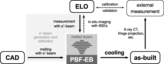
Figure 1. Schematic set-up for in-situ metrology in PBF-EB by ELO monitoring.
Download figure:
Standard image High-resolution imageHowever, the geometry obtained by ELO imaging only matches the as-built geometry to a certain extent. To enable reliable on-line decision-making based on ELO imaging, the degree of similarity must be high and known to the operator. This can be achieved by calibration and validation of ELO imaging against the as-built geometry. For this purpose the as-built geometry must be measured with an external device that should exhibit a higher accuracy than ELO imaging. Depending on the type and number of the geometrical features to be used for comparison, different techniques for external measurement are possible. In the current investigation, fringe projection and XCT were used for calibration and validation, respectively.
2.1. PBF-EB processing and ELO monitoring
Additive manufacturing and in-situ ELO monitoring were performed with the in-house developed PBF-EB system ATHENE. Its central component is a 6 kW electron beam gun by pro-beam GmbH & Co. KGaA (Gilching, Germany) that operates with an acceleration voltage of 60 kV. Using the standard configuration, the accompanying deflection system covers a build area of  mm2 and enables deflection speeds above 1000 m s−1. Feedstock material was plasma atomized Ti-6Al-4V ELI powder with particle size of 45–105 μm by Tekna Plasma Europe (Mâcon, France). The process was conducted in a controlled vacuum atmosphere of
  mbar helium pressure.
Parts were manufactured through layer-wise repetition of a PBF-EB build cycle that consisted of four major steps. In the first step a powder layer with a thickness of 50 μm was applied using a recoater system. The second step was preheating of the powder with a fast and defocused electron beam to maintain a process temperature of around 740 ∘C. The third step was selective melting of the current slice cross-section with a focused beam. A standard cross-snake hatching strategy with 90∘-rotation between layers was used for area melting. Further details on the chosen melting parameters for the two objects are given in the following sections. The fourth and last step was ELO imaging to acquire an image of the build surface before the next powder layer was applied and another run of the build cycle begun.
The ELO imaging step distinguishes the chosen build cycle from current standard PBF-EB build cycles. In this step a low-power electron beam scans linewise over a rectangular area. The kinetic energy of the beam electrons impinging the surface is not fully dissipated into heat but also converted to different kinds of secondary emission. The most important species in the current context are BSE, i.e. primary beam electrons reflected from build surface through elastic scattering with material's atom cores. These electrons may be captured with a BSE-detector and used to create an image in a similar way as performed in scanning electron microscopy. Since the number and direction of BSEs depends on material and topography of the surface, the intensity measured by the detector can be used to obtain an image contrast.
The sensor used for BSE detection was an annular copper plate which was located coaxial to the optical axis of the beam in central position above the build surface. The sensor and signal processing system was initially designed by pro-beam GmbH & Co. KGaA (Gilching, Germany) for applications in electron beam welding. In the current experiment a beam current of 3 mA was used to capture ELO images with a size of 1500×1500 px. The exposure area was set to 115 × 115 mm2 for the calibration experiment and to 70 × 70 mm2 for the validation experiment, leading to an instantaneous field of view of 77 and 47 μm px−1, respectively. The scan time for all images was set constant at 1.8 s. These imaging parameters are again summarized in table 1.
Table 1. ELO imaging parameters of the two PBF-EB build jobs associated with manufacturing of calibration and validation object.
| Calibration | Validation | |
|---|---|---|
| Image size | 1500 × 1500 px | |
| Exposure area | 115 ×115 mm2 | 70 × 70 mm2 |
| Instantaneous field of view | 77 μm px−1 | 47 μm px−1 |
| Image scan time | 1.8 s | |
2.2. Design and external measurement of calibration object
The purpose of the calibration object was the examination and enhancement of ELO imaging accuracy. The chosen design was a disc-shaped plate with concentric circular walls that had already been used in another investigation [28]. A sketch of the object is depicted in figure 2. The disc had a diameter of 115 mm, a thickness of 1 mm and was molten with a beam current of 25 mA and deflection speed of 10 m s−1. The hatch line spacing was 100 μm. Below the disc there was a columnar support structure with a height of 5 mm that connected the object to the steel base plate of the PBF-EB build job. The upper part consisted of 22 concentric circular walls and a central pin with a height of 1 mm. Between the walls there was a nominal spacing of 2.5 mm. Each circle was molten as single line with a beam current of 5 mA and a deflection speed of 1 m s−1. The central pin was molten with similar beam current and a spot residence time of 1 ms.

Figure 2. Sketch of the object built for calibration of ELO imaging.
Download figure:
Standard image High-resolution imageFor calibration purposes, the final position of the circular walls in real coordinates had to be determined by external measurement. Therefore the surface topography of the calibration object was measured with an optical 3D-scanner VR-5200 by Keyence Corporation (Osaka, Japan). The scanner works on the principle of fringe projection and is equipped with a movable stage to examine objects exceeding the optical field of view (7.6 × 5.7 mm2). The 2D height profile of the calibration object was measured along x- and y-direction through the center of the object. Precise orientation of the object with respect to the scanner was achieved by using two triangular markers on the base disc indicating the main axes (see also figure 2). The instantaneous field of view of the 3D-scanner was 7.4 μm px−1.
2.3. Design and external measurement of validation object
Figure 3 shows the chosen geometry for validation of the in-situ measurement approach. The specimen had a base-area of 10 × 10 mm2 and a height of 20 mm. The layer cross-sections were varied every 4 mm by cutting a stepwise increasing part of the cuboid geometry leading to different cross-sections shaped like the letter 'H'. Below the specimen there was a columnar support structure with a height of 5 mm. Choosing the build area center as coordinate system origin, the validation object's xy-centroid was put at a non-central position of x = 10 mm and  mm. The layers of the specimen were molten with a beam current of 6.7 mA, a deflection speed of 2.67 m s−1 and a hatch line spacing of 100 μm. It was manufactured in a PBF-EB build job together with a few other samples which are not relevant within the scope of this manuscript.

Figure 3. Sketch of the object built for validation of ELO imaging and in-situ measurement of geometrical and dimensional accuracy.
Download figure:
Standard image High-resolution imageTo validate the in-situ determination of dimensional accuracy, the as-built object also had to be measured externally. In contrast to the calibration object where only measurement of one surface was required, the validation object had to be captured in its full three-dimensional structure. Therefore, XCT was used as external measurement method for the validation object. The XCT system was a v|tome|x m 300 by GE Sensing & Inspection Technologies GmbH (Wunstorf, Germany). The x-rays were created with an acceleration voltage of 190 kV and a current of 60 μA. The acquired 2000 x-ray projection images were then used to reconstruct the three-dimensional density distribution with a voxel size of 10.00 μm.
2.4. Data processing for validation
Validation was performed by conducting a comparison between in-situ ELO imaging, XCT slice data and the CAD model in terms of geometrical and dimensional information. Figure 4 summarizes the processing of the geometrical data prior to comparison. Since the data was intended to be compared on a layer level, selection of the correct image from the stack of acquired ELO-images was the first step in case of ELO data post-processing. The image was then calibrated by including the deflection error as determined in the calibration experiment. Thermal shrinkage was considered by adjustment of the assumed pixel size from 46.7 to 46.3 μm. The decrease of 0.77% corresponds to the thermal strain created by cooling from 740 ∘C to 20 ∘C as found in literature [29] for material Ti-6Al-4V. To enable a more accurate comparison, the contour of the molten area was then extracted from the image by using a marching squares algorithm which is the 2D-case of the marching cubes algorithm [30]. The calculation was performed using the Python package scikit-image [31]. The algorithm requires a global threshold value to determine the desired interface. The gray value histogram of the ELO image showed a bimodal distribution with two very distinct peaks corresponding to molten material and powder bed. Hence, the required threshold value was simply set to be at 50%, i.e. the middle of the two peak maxima. This value is also denoted as 'ISO-50% threshold' [32]. Due to the non-central position of the manufactured part, consideration of deflection error and thermal shrinkage did not only change the dimensions but also the position of the part. To enable quantitative comparison between the three geometry variations, a translation was applied to the coordinates such as the molten area centroid fitted again its original position.

Figure 4. Data processing of the three geometry variations (ELO images, as-built part and CAD model) prior to comparison. Boxes on the same horizontal level indicate comparable processing steps between different data processing flows.
Download figure:
Standard image High-resolution imageIn case of XCT data, the reconstructed volume of the as-built part was first registered using the software suite VGSTUDIO MAX by Volume Graphics GmbH (Heidelberg, Germany) to compensate for slight rotation of the part during x-ray scanning. Afterwards, slice images in the xy-plane corresponding to the layers of the PBF-EB job were exported from the XCT voxel data set. The required effective layer thickness was calculated by using the as-built height of the validation object. The XCT slice image related to the desired layer was then also analyzed with the marching squares algorithm to determine the contour of the solid object. Again, the image exhibited a bimodal gray value histogram but a similar threshold in the center of the two peaks resulted in a visual overestimation of the solid volume. Thus, the global threshold was slightly adjusted from 50% to 66.67% between background and material peak to obtain a better result ('ISO-66.67% threshold'). Finally, a coordinate translation was applied to shift the centroid of the solid cross-section to the position indicated by the CAD model.
The third variation was the desired geometry as given by the CAD model. After slicing of the model with the chosen layer thickness, the contours of the required layer were exported for comparison. Since the CAD model was used as common reference system, no further translation of the obtained coordinates was required. The obtained polygons were then compared using the Python package Shapely [33] which is based on the GEOS library [34].
3. Results
3.1. 3D-scan of calibration object
The topographical information acquired with the 3D-scanner was used to investigate the dimensional accuracy of the as-built calibration object. Since the beam deflection system consisted of two deflection yokes in a 90∘ arrangement, the accuracy along the both main axes in x- and y-direction was evaluated. An overview of the scanned calibration object and the two evaluated axes is given in figure 5(a). The measured height profile along x- and y-direction shows distinct peaks which positions correspond to the position of the concentric circular walls of the calibration object (see figure 5(b)). The measured position of each peak was extracted and compared to the respective target position as given by the CAD model. The local deviation, i.e. the difference between actual and target position, is given for both axes in figure 5(c). Both curves show a positive and approximately linear slope which means that the calibration object was slightly larger than expected. For the most outer circular wall with a target diameter of 110 mm, the error in x- and y-direction was around 0.8 and 1.6 mm, respectively.

Figure 5. 3D-Scan of Calibration Object. (a) Overview scan with highlighted evaluation directions (x- and y-axis). (b) Height profile along both evaluation directions with distinct peaks marking positions of the concentric circular walls. Thin gray lines indicate the target position of the walls as given by the CAD model. (c) Deviation curves for both evaluation directions.
Download figure:
Standard image High-resolution image3.2. ELO-image calibration
The accuracy of the as-built calibration object was then compared to the accuracy obtained by non-calibrated ELO-imaging. As indicated in figure 1, an important factor that must be considered in this comparison is cooling of the PBF-EB part after the layer-wise build-up. The build process was conducted at 740 ∘C while the 3D-scan of the as-built object was performed at room temperature. Thus, significant thermal shrinkage of the object had to be included in the evaluation. This was performed by acquiring another in-situ ELO image of the build surface after cooling down of the build job. As shown by the authors in another investigation [28], it is possible to quantitatively deduce thermal shrinkage by evaluating ELO-images acquired at different temperatures.
Figure 6 contains the deviation curves created by thermal shrinkage of the calibration object and derived from in-situ ELO-images for both x- and y-axis. A detailed explanation on this measurement is given elsewhere [28]. To facilitate comparison, the deviation curves obtained from 3D-scanning of the final as-built object (see figure 5(c)) are also given in figure 6. In contrast to the as-built curves, the thermal shrinkage curves possess a negative slope since plain thermal contraction during cooling would lead to an object being smaller than defined in the CAD model. Given this data, it was then assumed that the measured as-built deviation curve at room temperature was a superposition of the actual deviation at processing temperature and thermal shrinkage. This is only an approximation but it is reasonable as long as the deviations are much smaller than the dimensions of the object.

Figure 6. Deviation curves of the calibration object along (a) x-axis and (b) y-axis. The final deviation of the as-built object as measured via 3D-scanning was approximated by a linear superposition of deviations created by inaccurate deflection during melting and thermal shrinkage during cooling.
Download figure:
Standard image High-resolution imageThe approximated deviation curves at processing temperature are also given in figure 6 and are denoted as 'deflection error'. The curves are linear and with positive slopes of 0.0138 and 0.0205 for x- and y-axis, respectively. The curves are steeper than the as-built deviation curves which means that, due to thermal shrinkage, the actual inaccuracy produced during PBF-EB manufacturing was even bigger than measured afterwards by 3D-scanning.
As already indicated by name, the reason for the observed inaccuracy was an inadequate parametrization of the the deflection system. First of all, the beam is deflected by a certain angle while the resulting deflection distance in the build plane depends on the working distance of the electron gun. In PBF-EB, this working distance is usually fixed but has to be set with high accuracy because otherwise a systematic error in beam deflection is created. This absolute error is zero in the center position (i.e. no deflection) and increases linear with higher deflection angle as observed in figure 6. Additionally, deflection in x- or y-direction is controlled by two separate deflection yokes. Within usual fabrication tolerances, the physical properties of the magnetic coils may exhibit variations which are leveled by adjusting the coil input signals. In case the chosen parameters are inappropriate, different accuracies in x- and y-direction will occur as observed with the investigated calibration object.
It is a remarkable yet logical finding that this deflection error as observed for the as-built object is not visible in the in-situ ELO-images. As already stated in another investigation [28] and again displayed in figure 7, the positions of the melt tracks in the original in-situ ELO-image match the target positions as defined by the CAD model rather well. The reason why the determined inaccuracy of the as-built object can not be derived from ELO images is that the required deflection performed during ELO imaging is suffering the same deflection error since it uses the same beam deflection system. In other words: the electron beam that melts a track at an inaccurate position also gathers BSEs at an inaccurate position during imaging and hence the error becomes invisible for ELO imaging.
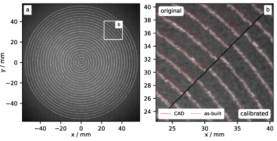
Figure 7. (a) ELO-image of the most upper layer of the calibration object. (b) Original and calibrated version of magnified image region. In the original image, the melt tracks show a good agreement with the positions given by the CAD model (solid lines). After calibration of the ELO-image, the melt tracks reflect the actual position as measured by 3D-scanning of the as-built part (dashed lines).
Download figure:
Standard image High-resolution imageThrough external measurement and the described evaluation of the calibration object, the deflection error was made visible and could be determined quantitatively. Furthermore, it could be assumed to be constant as long as the PBF-EB machines configuration remained unchanged. This enabled a computational calibration step with the goal of including the actual deviation artificially in any ELO-image, even if the image was acquired in another PBF-EB build job. The images were corrected by mapping the acquired pixel values to their actual spatial position and calculating a new ELO-image at the pixel original target positions through linear interpolation between known pixel values. As can be seen in figure 7(b), the resulting calibrated ELO-images were much closer to the actual situation inside the build chamber and thus a better basis for in-situ evaluation of manufacturing accuracy. However, it should already be stated that this approach is only to be considered a workaround for the current scientific investigation while better solutions for industrial application are discussed later.
3.3. Validation experiment
To validate the capabilities of in-situ ELO-imaging with respect to prediction of as-built dimensional accuracy, the geometry of the validation object was analyzed as described in the experimental section. Figure 8 shows exemplary image data obtained by (a) ELO imaging and (b) XCT scanning. The chosen layer was the central layer of the uppermost step section of the validation object (z = 23 mm). The direct comparison of the two images demonstrates the significantly higher spatial resolution of the XCT data which enables a detailed display of the surface roughness of the object. The rough contour is also visible in the ELO image of the molten area but is much more fuzzy. To evaluate the dimensional accuracy, the target contour as defined by the CAD model is marked as dashed line for both subfigures. For both images, the molten area seems to exceed the target contour of the object in most regions of the layer. The inaccuracy appears to be quite similar for both imaging methods but a quantitative comparison is difficult using these bitmaps.
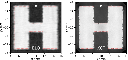
Figure 8. Qualitative comparison of (a) ELO image and (b) XCT slice for an exemplary layer (z = 23 mm) of the validation object PBF-EB build job. The dashed line in both images indicates the target contour as defined by the CAD model.
Download figure:
Standard image High-resolution imageTo enable the quantitative comparison, the contour of the solid area was extracted for both imaging methods as described above. Figure 9 shows the polygon comparison for the exemplary layer which was already investigated in figure 8. Each subfigure (a, b and c) compares two of the three different geometry variations. Table 2 contains the quantitative measures related to the investigation.
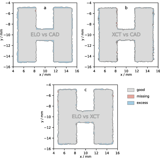
Figure 9. Quantitative comparison between the three geometry variations (ELO, XCT and CAD) of the exemplary layer (z = 23 mm).
Download figure:
Standard image High-resolution imageTable 2. Quantitative evaluation of dimensional agreement between the three different geometry variations for the PBF-EB layer depicted in figure 9.
| ELO vs CAD | XCT vs CAD | ELO vs XCT | |
|---|---|---|---|
| Reference area | 73.4 mm2 | 73.4 mm2 | 76.9 mm2 |
| Good | 73.2 mm2 (99.8%) | 72.6 mm2 (99.0%) | 76.4 mm2 (99.3%) |
| Missing | 0.2 mm2 (0.2%) | 0.8 mm2 (1.0%) | 0.5 mm2 (0.7%) |
| Excess | 7.4 mm2 (10.0%) | 4.3 mm2 (5.9%) | 4.2 mm2 (5.4%) |
| Total Agreement (Jaccard Index) | 90.7% | 93.5% | 94.2% |
Figure 9(a) displays the accuracy of the ELO image with respect to the cross-section obtained from the CAD model. It shows that the molten area does not show severe deviations from the general shape of the target cross-section and the reference area (73.4 mm2) is correctly molten to 99.8%. Only in a few locations and a small area (0.2%) the desired material consolidation is missing. Nevertheless, inaccuracies in the border region of the area are clearly visible. The edges are not straight but exhibit roughness in the xy-plane. Furthermore, the molten area seems to be slightly bigger than aimed for, leading to a shell of excess material (10.0% of the reference area) along the contour of the cross-section. The total agreement between both regions is quantified by using the Jaccard similarity index [35]. As given by equation (1), the Jaccard index J is defined as the ratio between the intersection and the union of region Ω and reference region  . The norm
  represents the area of the (sub-)region. Thus, the total agreement between ELO image and CAD cross-section is found to be 90.7%:
Figure 9(b) compares the data obtained from XCT scanning to the CAD model. The evaluation shows that the XCT slice image exhibits a higher amount of missing material (1.0%) which is mainly located in one edge region of the part. However, the amount of excess material for XCT scanning (5.9%) is significantly lower than seen for ELO imaging. Thus, the total agreement shows a slightly higher value of 93.5%.
Using the CAD model as a reference only gives information about how accurate the layer is molten with respect to the desired geometry. Similar values obtained for ELO and XCT data do not necessarily result from a high similarity between both imaging methods because deviations might be found in different locations of the molten layer. Hence, the third comparison is drawn directly between the ELO and XCT data where the latter acts as reference area. As shown in figure 9(c) the two very different imaging approaches show a remarkable good agreement. The intersection area is similar to the previous comparisons (99.3%) while the amounts of missing (0.7%) and excess material (5.4%) are relatively low. This results in a high total agreement of 94.2%.
A detailed look on figure 9(c) shows that the high agreement is not a random calculation artifact. Despite the erratic course of the contour, many of its characteristic intrusions and extrusions can be found in both imaging approaches. As a result, the local deviation between ELO and XCT data stays rather small everywhere along the contour. To further characterize the agreement between ELO and XCT data, this local deviation may be calculated as a signed distance for every vertex of the contour. Figure 10 shows the deviation profile obtained from this evaluation. It starts in the upper left corner of the molten area (close to x = 5 mm and  mm) and follows the contour in clockwise direction. Again, it shows that the major part of the deviation is caused by excess, i.e. molten areas which are found in ELO imaging but not in XCT scanning. It also shows that, apart from few extreme values for negative (
 m) and positive (253 μm) deviation, the greater part of the profile is relatively close to zero with an average deviation of 55 μm. The average absolute deviation of 67 μm is only slightly higher.

Figure 10. Deviation between ELO and XCT data along the contour of molten area. The profile starts in the upper left corner of the molten area in figure 9(c) (close to x = 5 mm and  mm) and follows the contour in clockwise direction. The average deviation is 55 μm.
Download figure:
Standard image High-resolution imageThe high agreement between ELO and XCT data was not only found for the exemplary layer but for the major part of the validation object. Figure 11 displays the Jaccard similarity indices of the three pairwise comparisons for all layers of the specimen. The Jaccard index between ELO and XCT data is found to be almost everywhere at around 95%. However, it also indicates a lower similarity in the first layers of the part and in regions where the cross-section is abruptly changing due to the staircase structure of the object. The lower similarity in these regions originates from a lower similarity between the as-built part (i.e. XCT) and the CAD geometry which can not be found in the ELO data. It may be noted that both index curves involving the CAD geometry display a step-wise decrease with changing cross-section geometry. The reason is the increasing contour-to-area ratio of the CAD cross-sections. Since deviations are mainly observed along the contour, the similarity with the CAD geometry decreases with increasing contour length. However, the Jaccard index between ELO and XCT data is hardly affected by this effect which underlines the robustness of the observed similarity.

Figure 11. Jaccard indices of the three pairwise geometry comparisons for all layers of the validation object.
Download figure:
Standard image High-resolution image4. Discussion
Within the current investigation, in-situ evaluation of dimensional accuracy by ELO imaging shows a high agreement with XCT scanning of the as-built part. The average deviation between ELO and XCT imaging was determined to be well below 100 μm. This is a remarkable result considering the comparatively low ELO resolution which results from an electron beam diameter of around 400 μm. It is also a highly relevant finding since it means that ELO imaging may be used to closely predict and control the dimensional accuracy of the as-built PBF-EB part. The high agreement could only be achieved by including several factors into the evaluation. Some other factors could not be reliably assessed or quantified and thus limit the observed agreement. In the following sections, both incorporated and limiting factors are discussed in more detail.
4.1. ELO image post-processing
Thorough post-processing of the ELO images is crucial for the comparison with XCT and CAD data (see figure 4). As shown for the calibration object, the raw ELO images do not necessarily display the actual part geometry inside the build chamber. In case the deflection system is not parametrized precisely, the cross-sections are molten incorrectly. However, the resulting inaccuracy is not depicted by the ELO imaging system due to its own dependence on the deflection system accuracy. This issue was solved in the current investigation by quantifying the deflection error once and then including it into other ELO images by a mathematical correction. This operation returns much more accurate ELO images with respect to the as-built geometry inside the chamber, as long as the parametrization of the deflection systems remains unchanged. However, the inaccuracy of the manufactured part with respect to the target CAD geometry is not solved with this approach. This limitation was not a problem for the current investigation because its focus was only on the assessment of in-situ metrology capabilities of ELO imaging. The applied workaround enabled usage of already acquired data without the necessity of a re-parametrization for the deflection system and a costly repetition of several experiments. Nevertheless, it should be highlighted that for industrial production where manufacturing of high-quality parts is the main objective, the workaround applied in this investigation is not advisable. Instead, a thorough parametrization of the deflection system should be conducted in advance to avoid errors in the first place. That approach inherits the benefit of improving the accuracy of both the manufactured part and the acquired ELO images.
A second important factor to consider is thermal shrinkage of the part during cooling down of the build job. Caltanissetta et al stated that layer-wise imaging could not capture thermal shrinkage and hence in-situ measurement would not be representative of the as-built part [15]. However, as shown in another investigation [28], thermal strain created during cooling down in PBF-EB can be approximated quite well using data obtained from non-AM literature. Thus, thermal shrinkage was included into the current evaluation since that is the only possibility to validate and apply the approach for multiple layers, i.e. real parts. The thermal strain of −0.77% which was corrected in the current investigation appears to be small and actually only has a small influence on the given result. Nevertheless, this assessment is bound to two specific characteristics of the chosen build job and may not be generalized. First, the investigated distances were rather short due to the relatively small size of the validation object (10 × 10 mm2). For larger parts using the full build area (130 × 130 mm2), thermal shrinkage may create inaccuracies of more than 1 mm. Second, the effect strongly depends on the properties of the feedstock material. Many other metal alloy systems exhibit a significantly higher coefficient of linear thermal expansion (up to a factor 3) than the investigated titanium alloy Ti-6Al-4V. Additionally, the PBF-EB processing temperature which must be adjusted for every material may be much higher (up to 1100 ∘C) which increases thermal shrinkage during cooling down furthermore. Thus, consideration of thermal expansion can be crucial for making accurate predictions with respect to dimensional accuracy and hence must be included into the evaluation.
The third important factor during post-processing of the ELO images is a suitable translation of the determined coordinates to enable a reasonable comparison. Beam deflection for melting and ELO imaging is supposed to follow the same coordinates system as defined in the CAD model. However, deflection error and thermal shrinkage create a displacement of the molten volume. Since a plain displacement of the manufactured part within the build chamber does not affect its dimensional accuracy, the effect should be compensated for prior to comparison. Hence, to obtain a more accurate result, the translation of the molten area's centroid from its original position was calculated and used to back-translate the entire area to its original position. This analytical operation was favored over other possible approaches (e.g. manual or best-fit registration) because it does not rely on an external reference (e.g. the CAD model) and thus preserves the independence and reliability of the acquired ELO image data.
4.2. Data comparison
To conduct the comparison, an iso-contour extraction algorithm was applied to the ELO and XCT image data. This approach was favored over applying the threshold values directly to the pixel data and conducting a pixel-wise comparison as proposed by Wong [24]. The reasons was the goal to minimize artifacts related to very different pixel sizes of ELO and XCT and to avoid information loss related to a grid discretization of CAD data. Edge detection and segmentation was performed by applying a global threshold value which was chosen by calculating the very simple ISO-50% value from the gray-level histogram. Due to the high contrast between molten area and powder bed, as well as the absence of disturbing reflections, the approach nonetheless returned excellent results. This highlights a huge advantage of ELO imaging over common light-optical imaging of the build surface where extensive efforts have to be made to develop robust algorithms for image segmentation [12, 13, 15–17]. Nevertheless, in the future, more sophisticated adaptive thresholding algorithms might also be tested on ELO images to further enhance the quality of surface extraction.
Three comparisons were used to identify deviations between the three geometry variations. The deviations were divided into two classes which are missing and excess material. This distinction is not only useful to analyze the origin of the deviations but also has a high practical relevance. Depending on its location, excess material might be removed by post-processing to obtain high accuracy parts while inaccuracies created by missing material can hardly be corrected.
In total, the investigated cross-section of the validation object was molten quite correctly and it did not exhibit any features with severe deviation. The observed inaccuracy was mainly observed as profile roughness along the contour of the molten area. This may be explained with the non-stationary conditions found in these regions due to changing beam velocity and the complex interface between molten material and the particles of the surrounding powder bed. In comparison with the CAD model, both ELO and XCT data showed a large amount of excess material which was found in a shell-like arrangement around the desired cross-section. The reason for this shell is probably the absence of a beam diameter compensation during melting. Due to its finite diameter of approximately 400 μm, the electron beam overshoots the desired area when its center reaches the contour. The observed excess material shell had a thickness of 200–300 μm which is in well agreement with the half diameter of the beam.
The area and area fraction of the deviation regions were measured to obtain quantitative measures for the accuracy of ELO imaging and the as-built part. It should be noted that the size of these quantities strongly depends on the size and especially the surface-to-volume ratio of the target geometry since deviations were mainly observed along the contour of the molten area. Thus, comparing areas and area fractions is only reasonable for similar target cross-sections, e.g. during optimization of scan strategy parameters. The same holds true for the applied Jaccard Index and the comparable Sørensen-Dice index [36, 37] which were also used in other investigations to assess the performance of image segmentation algorithms [15, 17].
As an alternative evaluation approach, the local profile deviation along the contour was calculated which is less dependent on the size and shape of the geometry. Since it gives the signed distance to the reference geometry for every point along the contour, it may be used to extract the average deviation or extreme values either for the whole part or only selected regions. As shown by Pagani et al, this kind of measure is an excellent base for in-process quality control when the CAD model is used as a reference [16]. The obtained graph resembles a profile roughness plot and may actually interpreted in similar way since the deviation between the contour of the as-built part (XCT data) and the CAD model creates roughness within the xy-plane. Together with the roughness that may be measured along the build direction (i.e. z-axis), it defines the total roughness of the as-built PBF-EB surface. Surface roughness often is an important and critical aspect of AM parts. Since ELO imaging shows a good agreement with the as-built geometry, it might be used for in-situ control and optimization of surface roughness. As shown in the comparison with the XCT slice image, the resolution of the contour profile might be further increased by enhancing the resolution of the ELO image, e.g. by using a smaller beam diameter.
The total agreement between ELO and XCT data is remarkably high but yet well below 100%. Beside the different imaging resolutions, there are additional limiting factors to be considered. First, ELO imaging only depicts the surface of the PBF-EB build job for every layer. As shown in figure 12(a), this surface almost always is remolten with the subsequent layer(s). Therefore, most ELO images only display an intermediate state which affects the final as-built geometry, but not exclusively. This inevitably impairs the accuracy of the predictions made via ELO-imaging, not only in terms of dimensional accuracy but also with respect to internal defects which was already shown in another investigation [25]. Further research is necessary to completely evaluate the prediction capabilities of ELO imaging with respect to the different geometrical features of the parts. As an example, first experiments indicated that the presence of upskin and downskin regions may strongly affect the achievable accuracy. This is also observed in figure 11 where the similarity between ELO and XCT data is significantly lower for the bottom layers and the cross-section transition layers of the validation object. The causes of these deviations are probably thermal stress-induced processes which take place during melting of subsequent layers. As already stated by Caltanissetta et al, thermal stress-induced distortions can hardly be captured by layer-wise imaging [15]. However, it should be noted that thermal stresses are significantly smaller in PBF-EB than in PBF-LB due to lower thermal gradients and cooling rates [38].

Figure 12. Surface roughness along build direction as a limiting factor for the agreement between ELO and XCT data. (a) Schematic interrelation between surface roughness and layer imaging via ELO and XCT. (b) XCT slice along build direction which displays the surface roughness of the as-built part.
Download figure:
Standard image High-resolution image
Nevertheless, the deficit in agreement between ELO imaging and as-built part may not only be attributed to limitations of ELO imaging. Also the as-built geometry which is used as reference may only be determined with limited accuracy. During the evaluation, the data obtained from XCT scanning was treated as 'ground truth' for the as-built part. Considering its small voxel size of only 10 μm this was a plausible assumption but only as long as the XCT geometry was treated as a whole. However, the layer-wise comparison with ELO and CAD data required the extraction of single XCT slices. Each of these selected XCT slices was supposed to represent a distinct layer of the PBF-EB build job. The selection process entails some uncertainty since a molten layer has a thickness that exceeds the voxel size of the XCT scan. Furthermore, the effective layer thickness of the as-built part, which is required to relate XCT slices and PBF-EB layers, is not equal to the processing layer thickness of 50 μm. Primarily, the effective layer thickness is affected by thermal shrinkage of the part during cooling down. The new value was estimated by measuring the actual height of the sample and dividing the value by the number of layers. This calculation delivered an effective layer thickness of 49.5 μm which equals a thermal strain of −1%. This value is close to the theoretical thermal strain of −0.77% which was used for correction of the ELO images. Nevertheless, it only remains an estimation and a small error per layer accumulates with increasing layer number. Thus, a precise adjustment and data registration becomes even more important for parts with a larger build height. This estimation results in an uncertainty while choosing the optimal z-coordinate for XCT slice extraction. As shown in figure 12(b), the as-built PBF-EB part exhibits a high surface roughness along the build direction. Its maximum roughness depth is approximately 250 μm. Hence, a small variation in the z-coordinate may shift the contour position within the xy-plane by this maximum roughness depth. A comparison with figure 10 shows that this consideration is in excellent agreement with the observed deviation where a maximum excess distance of 253 μm was observed. Also the predominance of excess material in the comparison between ELO and XCT data may be explained with this approach. As depicted in figure 12(a), the surface roughness along the z-direction is partly created by the curvature of the molten layer due to the melt pool temperature profile. ELO imaging always displays the surface of the molten layer which has the largest extension. On the other hand, the XCT slices are extracted in varying position within the layers due to the aforementioned uncertainty in calculating the respective z-coordinate. Therefore, the size of the molten area in the XCT slice has a high probability of being smaller than its ELO equivalent leading to the observed dominance of excess material in the prediction.
4.3. Application
The presented results suggest the application of ELO imaging for making in-situ predictions on the dimensional accuracy. This would give several advantages over conventional approaches. First, there is a big economical benefit because a subsequent measurement of the as-built parts requires high-level metrology equipment and trained operators. This leads to high capital and operating expenditure, especially when using XCT systems. This is the reason why the full inspection of as-built AM parts currently is limited to high-cost applications with elevated quality requirements. In comparison, ELO imaging is very economic since the related hardware is inexpensive and the data record is conducted automatically during the PBF-EB process. Furthermore, ELO imaging enables in-situ quality control, i.e. the detection of errors during processing. Compared to post-process quality control, this may spare additional resources by enabling early intervention through adjustment or deactivation of low-quality parts.
XCT scanning is currently seen as the most versatile method to inspect as-built AM parts [5] and may return very accurate measurements. Also the current investigation has shown that the obtainable resolution is much higher for XCT than for ELO imaging. Therefore, for critical parts, an additional XCT scan of the as-built part may still be demanded to identify small-scale defects. However, it must be noted that the resolution of XCT is limited by the attenuation of the x-rays used for scanning. Larger geometries and higher material densities lead to a strong attenuation which must be compensated by increasing the XCT power. This usually leads to an increasing x-ray spot size and thus decreasing spatial resolution. Additionally, due to a limited x-ray detector size, the distance between sample and detector must also be increased for larger geometries which reduces magnification furthermore. In the current investigation, the validation object was relatively small (10 ×10 × 20 mm2) and the density of Ti-6Al-4V is rather low (4.4 g cm−3) compared to other alloys used for metal AM. This conditions enabled a low XCT voxel size of 10 μm. However, realistic PBF-EB parts may possess dimensions above 100 mm and common alloys in use show densities above 8 g cm−3. Together with the non-linear character of x-ray attenuation, this leads to a drastic decrease of the achievable XCT resolution.
The spatial resolution of ELO imaging mainly depends on the diameter of the electron beam and thus is expected to be much less susceptible to the size of the part. Additionally, the density of the feedstock material does not affect the quality of the ELO images. It may therefore be expected that ELO imaging could outperform XCT scanning for large-scale or high-density parts which are manufactured for technical applications. As alternative to XCT, light-optical 3D scanners might be less susceptible to size and density of the part. However, these devices are not capable of fully inspecting complex parts with undercuts and often suffer problems when measuring reflective metallic surfaces. Due to its layer-wise approach, ELO imaging is capable of measuring undercut regions, independent of geometry and size of the part. Additionally, the ELO images are free of reflections and instead show a high contrast between molten surfaces and powder bed which enables reliable and robust measurements.
5. Conclusions
It was shown that ELO imaging offers a new possibility for in-situ metrology in PBF-EB and to predict the dimensional accuracy of the as-built part. However, to obtain high quality results a thorough post-processing of ELO images is required. This post-processing includes considerations with respect to accuracy of beam deflection, thermal shrinkage of the part during cooling down and data set registration.
To demonstrate the capabilities of the ELO imaging approach, a cross-section of an exemplary part was investigated by comparison with CAD and XCT data. The geometrical accuracy obtained by ELO imaging showed a high agreement with the measured accuracy of the as-built part (above 90%). The average local deviation between in-situ and ex-situ measurement was below 100 μm. The maximum local deviation was equal to the surface roughness of the part, probably due to the uncertainty associated with the mapping between ELO images and XCT slices. In total, ELO imaging tended to predict a slightly larger volume than actually measured for the as-built part. The reason for this is seen in the limitation of ELO imaging to only display the surface of the build area.
In summary, the high agreement between ELO images and the geometry of the as-built part is very promising. The technical and economical advantages of ELO imaging by far outweigh its limitations. Thus, measurement of geometrical and dimensional accuracy via ELO imaging is suggested to be applied for in-situ process and quality control of PBF-EB. Depending on the part's geometry and application, it may complement or even replace post-process inspection tools like XCT scanning.
Data availability statement
The data that support the findings of this study are available upon reasonable request from the authors.
Disclosure statement
The authors declare that there is no conflict of interest.
Authors' contributions
Christopher Arnold: conceptualization, methodology, software, investigation, formal analysis, writing—original draft; Carolin Körner: conceptualization, supervision, writing—review and editing, funding acquisition.
Acknowledgments
The authors gratefully acknowledge funding by the Dobeneck-Technologie-Stiftung and the European Space Agency (ESA Contract No. 4000124431/18/NL/MH/mg). This project has received funding from the European Union's Horizon 2020 research and innovation programme under Grant Agreement 820774 ('MANUELA').