
Abstract
Silicene, a graphene-like 2D material made from Si atoms, has been fabricated and studied for its promising applications in micro/nanoelectronics. For the reliable function of silicene devices, it is important to investigate silicene's mechanical properties. In this study, the authors conducted density functional theory (DFT) simulations of mechanical tests of silicene and investigated the elastic modulus and mechanical response such as structural transformation. In addition, the authors optimized the Tersoff potential parameters using a gradient-based minimization with a grid search method in hyperdimensional parameter space, to match the DFT calculation results in the elastic regime. With the new parameter set, the elastic moduli of silicene in the zigzag (ZZ) and armchair (AC) directions were computed with molecular statics (MS) simulations and compared with those of other Si interatomic potential models and DFT results. In addition, uniaxial tensile tests along the ZZ and AC directions were performed to examine how far the Tersoff model is transferable with our new parameter set to describe the nonlinear mechanical behavior of silicene. The results of uniaxial tensile tests suggest that the angle penalty function in the Tersoff model needs to be modified and that the stress–strain curve predicted with this modification shows improvement compared to the original function.
Export citation and abstract BibTeX RIS

Original content from this work may be used under the terms of the Creative Commons Attribution 4.0 licence. Any further distribution of this work must maintain attribution to the author(s) and the title of the work, journal citation and DOI.
This article was updated on 20 May 2021 to correct the name of the second affiliation (Kyong Hee was changed to Kyung Hee).
1. Introduction
Silicene, which consists of Si atoms, has a single layer of hexagonal honeycomb structure [1–3]. Unlike graphene, the bonds between Si atoms are sp2–sp3 hybridization and the atoms are puckered rather than perfectly aligned in a single plane [4]. Due to its buckled structure, the properties of silicene can be easily tuned by an electric field or external force [5–7]. Therefore, silicene has extra potential to be applied in the electronic device industry.
Mechanical deformation can develop during the fabrication or operation of silicene-based electronic components such as transistors [8] or light-emitting diodes [9]. For example, silicenes that are synthesized by epitaxial growth on Ag or Ir substrates reportedly have a different structure from free-standing silicene [10, 11]. Structural changes or deformation can affect the performance of applications by changing the electronic band structure of silicene [12]. Therefore, it is important to study the mechanical stability and properties of silicene for its reliable application.
Silicene has been reported as a highly reactive material that is easily oxidized in ambient conditions. Therefore, the encapsulation process of silicene with Al2O3, Al, or transition-metal dichalcogenide layers has been developed for its chemical stability [13, 14]. By performing mechanical test experiments with encapsulated silicene, we may indirectly deduce the mechanical properties of silicene using the mechanics of composite materials. On the other hand, we can directly obtain the mechanical properties of free-standing silicene from atomistic simulations such as density functional theory (DFT) and molecular statics or dynamics (MS/MD). DFT is regarded as a more accurate tool than MS/MD since it predicts material behavior based on the explicit evaluation of electronic structure. DFT studies have been actively conducted on the mechanical properties (e.g. in-plane moduli and Poisson's ratio) of silicene [15, 16]. However, due to its heavy computational cost, DFT calculation is generally not feasible for large-scale simulations such as bending and wrinkle formation of 2D materials on the substrate, which would include thousands of atoms. Instead, researchers have resorted to MS/MD to study the mechanical behavior of silicene. For example, elastic constants and fracture toughness were investigated using the ReaxFF model at 10 K [17]. The bending modulus of silicene was also calculated with the same model [18]. Simulations with the modified embedded atom method (MEAM) model were conducted to study fracture behavior in tensile tests [19]. Nanoindentation simulation by the Tersoff model was done using a diamond ball indenter to study the mechanical response of single-layer pristine silicene [20]. The same group investigated various mechanical properties of silicene via MD simulations of tensile tests [21]. Furthermore, the fracture strength and toughness of polycrystalline silicene were studied [22, 23] using a Stillinger–Weber model [24].
It should be carefully pointed out that the mechanical properties of silicene as predicted by the aforementioned MS/MD studies are questionable because most models were developed to reproduce the mechanical properties of bulk Si rather than silicene. The main goal of this study is to investigate the mechanical behavior of silicene using DFT simulation, which is more accurate than MS/MD, and to develop a reliable potential model that can be used for large-scale simulation for future study.
2. DFT study of the mechanical behavior of silicene
Prior to the parameter optimization of the potential model, DFT calculations were performed in the first instance to study the reference structures of silicene such as the minimum-energy structure and to investigate the mechanical behavior in tensile tests. This study is important in that not only are the results themselves physically meaningful but also the results can be used as reference data for the development of potential models.
2.1. Silicene structure and its elastic properties
The supercell of silicene is indicated by the dotted line in figure 1(a). The supercell contains four Si atoms and its x and y axes correspond to the zigzag (ZZ) and armchair (AC) directions, respectively. Two metastable structures were reported in Cahangirov et al [25]: buckled (Hex.2b) and planar (Hex.2p) structures the side views of which are presented in figures 1(b) and (c), respectively. According to DFT calculations, Hex.2b is more stable than Hex.2p in terms of cohesive energy. The DFT row in table 1 lists the lattice constant a, buckling parameter Δ, and cohesive energy of each relaxed structure.

Figure 1. (a) Schematic of the full atomistic model of silicene with the zigzag (ZZ) direction along the x axis and the armchair (AC) direction along the y axis. The supercell used for DFT calculations is shown by the dashed black line. The side views of (b) buckled (Hex.2b) and (c) planar (Hex.2p) structures depict the lattice constant a and buckling parameter Δ. Δ = 0 in the planar structure while Δ > 0 in the buckled one. Table 1 lists the lattice constant a and the buckling parameter Δ.
Download figure:
Standard image High-resolution imageTable 1. Structural parameters of silicene relaxed with different potential models at 0 (K): structure—Hex.2b (=Buckled), Hex.2p (=Planar), Tetra.1p (=Rectangular), Hex.1p (=Hexagonal), lattice constant a, buckling parameter Δ, and cohesive energy Ec in 2D.
| Potentials | Structure | a (Å) | Δ (Å) | Ec (eV/atom) | |
|---|---|---|---|---|---|
| MS | EDIP [26] | Hex.2p | 4.02 | 0 | 4.010 |
| Tersoff [27] | 3.99 | 0 | 3.911 | ||
| MA95 [28] | 3.99 | 0 | 3.912 | ||
| MA2013 [29] | Hex.2b | 3.84 | 0.78 | 4.210 | |
| MEAM [30] | 3.73 | 0.91 | 3.477 | ||
| SW92 [31] | 3.84 | 0.78 | 3.473 | ||
| SW2014 [24] | 3.81 | 0.43 | 2.691 | ||
| ReaxFF [17] | 3.80 | 0.70 | 3.450 | ||
| This study | Hex.2p | 3.94 | 0 | 4.836 | |
| Hex.2b | 3.87 | 0.45 | 4.855 | ||
| Tetra.1p | 2.34 | 0 | 4.629 | ||
| Hex.1p | 2.40 | 0 | 4.785 | ||
| DFT | GGA | Hex.2p | 3.90 | 0 | 4.764 |
| Hex.2b | 3.87 | 0.45 | 4.784 | ||
| Tetra.1p | 2.31 | 0 | 4.520 | ||
| Hex.1p | 2.49 | 0 | 4.457 |
DFT calculations were carried out with the Vienna Ab initio Simulation Package (VASP) [32–35] in which a projector augmented-wave method was used as a plane wave basis set. We used the generalized-gradient approximation (GGA) for the exchange-correlation functionals to compare the results between the two. A 25 × 25 × 1 k-point mesh for the Brillouin zone was sampled using the Monkhorst–Pack scheme. The length of the supercell in the z direction was chosen to be 20 Å (or Lz = 20 Å), which was long enough to minimize the image interaction. The energy cutoff was extended to 500 eV for precise calculations and the convergence criterion was selected to be 10−5 eV for electronic relaxation and 10−4 eV for ionic relaxation between relaxation steps. Every structure was relaxed with an energy minimization method, e.g. the Blocked–Davidson scheme [36].
We conducted three types of mechanical test simulation with a buckled silicene structure to calculate the elastic properties: Young's modulus (Y2D), Poisson's ratio (ν), and bulk modulus (B2D). The details of the calculation method are described in the electronic supplementary materials S1 (available online at stacks.iop.org/NANO/32/295702/mmedia). The bottom row of table 2 lists the 2D Young's modulus (Y2D), Poisson's ratio ( ), and 2D bulk modulus (B2D) of buckled silicene from a DFT calculation of mechanical tests. Y2D in the ZZ and AC directions are 61.7 (N m−1) and 61.8 (N m−1), respectively, and
  is obtained as 0.31 regardless of the direction. The elastic constants are similar to previous DFT calculations [5, 7, 15, 16, 37]. Since the 2D Young's moduli along the ZZ and AC directions are almost identical, the isotropic behavior of silicene is expected under small deformations. For isotropic 2D material, B2D is related to Y2D and
  as in equation (1) [38].

Table 2. 2D Young's modulus Y2D, Poisson 's ratio  and 2D bulk modulus B2D of buckled silicene. In the references with the asterisks (*), isotropy is assumed.
| Y2D (N m−1) |

| ||||||
|---|---|---|---|---|---|---|---|
| Potentials | ZZ axis | AC axis | ZZ axis | AC axis | B2D (N m−1) |

| |
| MS | MA2013 [29] | 52.6 | 52.6 | 0.03 | 0.03 | 27.4 | 0.993 |
| MEAM [30] | 26.7 | 26.8 | 0.22 | 0.22 | 17.3 | 0.988 | |
| SW92 [31] | 37.7 | 37.7 | 0.17 | 0.17 | 22.7 | 1.004 | |
| SW2014 [24] | 39.6 | 39.6 | 0.11 | 0.11 | 22.3 | 0.996 | |
| ReaxFF [17] | 41.6 | 41.6 | 0.26 | 0.26 | 28.2 | 0.996 | |
| This study | 59.8 | 59.8 | 0.17 | 0.17 | 36.0 | 0.997 | |
| DFT | Qin et al [5]* | 63.0 | 63.0 | 0.31 | 0.31 | · | · |
| Zhao [15] | 60.06 | 63.51 | 0.41 | 0.37 | · | · | |
| Peng et al [16]* | 63.8 | 63.8 | 0.33 | 0.33 | · | · | |
| Goli et al [37] | 66.72 | 67.63 | · | · | 40.11 | · | |
| This study—GGA | 61.7 | 61.8 | 0.31 | 0.31 | 45.0 | 0.994 | |
Thus, we checked the ratio of  and B2D and the value in the bottom-right cell of table 2 is 0.994, which is close to 1 and thus indicates that silicene is isotropic for small strain.
2.2. Tensile tests in large deformation
Uniaxial tensile tests were carried out for silicene of buckled and planar structures up to ε = 30% in both the ZZ and AC directions. Figure 2 presents the per-atom energy curves and the buckling parameter (Δ). When the buckled silicene is under tension in the ZZ direction, a structural transition to the planar one is observed at ε11 = 21% (green arrow in figure 2(a)), after which the per-atom energy curve (solid black line) of the buckled structure is overlapped with that of the planar one (solid red line). The transition strain of ε11 = 21% is clearly captured in figure 2(b) as the value of the buckling parameter is less than 10% of the initial value (Δ0 = 0.45 Å). This result is different from that reported by Peng et al [16], according to which the buckling parameter is maintained as about 75.6% of Δ0 even at ε11 = 18.3%. Similarly, Mortazavi et al also reported that the buckling parameter decreases only by 17.0% at ε11 = 9.5% [39]. The secret to the difference between our results and the previous studies lies in the loading condition. In Peng et al [16] and Mortazavi et al [39] the silicene was under a uniaxial stretch condition, while it is under a uniaxial tensile condition in this study. We were able to reproduce previous results when we repeated the simulations under a uniaxial stretch condition. At ε11 = 25%, the solid lines in figure 2(a) abruptly drop and increase again, implying that another structural change may occur. Indeed, the hexagonal lattice structure transforms into a rectangular lattice structure at ε11 = 25% in figure 3(a). On the other hand, when silicene is under tensile loading along the AC direction, the buckling parameter only decreases by about 16% until ε22 = 21% (see figure 2(b)) and the structure remains planar at a large strain of ε22 = 40% in figure 3(b). Evidently, in figure 2(a), the per-atom energy of the planar structure (dashed red line) is always larger than that of the buckled structure (dashed black line) in the range of ε22 ≤ 30%. In figure 3(b), the atomic bond, parallel to the AC tensile direction, is stretched from lbond = 2.778 Å to 3.348 Å at ε22 = 40%, while other bonds experience a slight increase of 0.005 Å. This separation tears silicene into several 1D zigzag Si chains. Similar fracture behavior for hexagonal boron nitride was reported in the tensile tests along the AC direction [40].
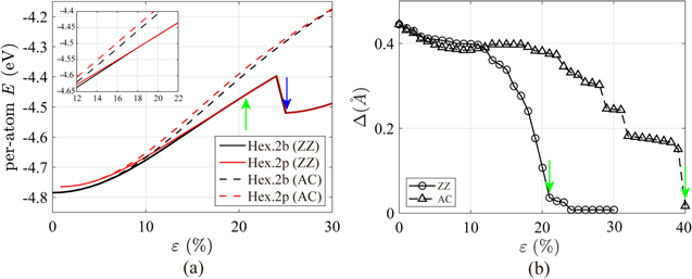
Figure 2. DFT calculations of (a) per-atom energy versus strain curves from the uniaxial tensile simulations of silicene (in the Hex.2b and Hex.2p structures) along the zigzag (ZZ) and armchair (AC) directions; the green arrow indicates the transition strain at which the buckled structure (Hex.2b) becomes planar (Hex.2p) in the tensile test along the ZZ direction. The blue arrow denotes the transition strain at which the planar structure (Hex.2p) transforms into a rectangular one (Tetra.1p). (b) Buckling parameter (Δ) versus tensile strain (ε). Green arrow denotes the transition strain, as in (a).
Download figure:
Standard image High-resolution image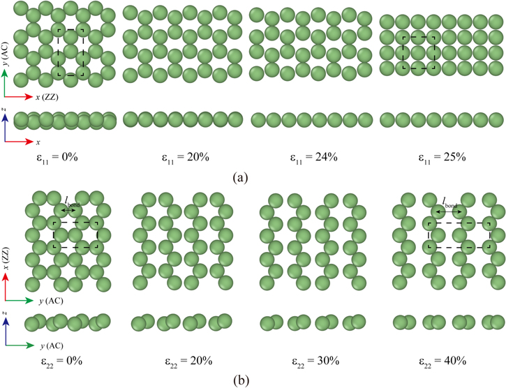
Figure 3. Structural change in DFT simulations of uniaxial tensile tests (a) In tensile tests along the ZZ direction, the lattice structure changes from buckled hexagonal (Hex.2b) to planar hexagonal (Hex.2p) at ε11 = 21% and later into a rectangular one (Tetra.1p) at ε11 = 25%. (b) In the tensile test along the AC direction, the structure becomes planar only after ε22 = 40%. Silicene sheet shows splitting into 1D zigzag Si chains.
Download figure:
Standard image High-resolution image3. Tersoff potential parameter optimization
In section 2.2, it is observed that silicene can have multiple metastable structures, which made the authors choose Tersoff [27] among existing Si potential models for parameter optimization because this model has the ability to predict various structures ranging from a 3D diamond cubic structure to FCC with relatively simple functions due to its bond-order nature. The authors intended for the optimized model to predict 2D polytypes of Si to reproduce structural changes of silicene predicted in DFT simulations of tensile tests.
3.1. Parameter optimization method
There are 13 adjustable parameters (A, B, λ1, λ2, λ3, α, β, n, c, d, h, R, and D) in the Tersoff model [27] but we keep α, R, and D and only consider the remaining 10 parameters during optimizations (the equations of the Tersoff model are in the supplementary S2). Following the philosophy of the original Tersoff model, the bond-order function bij in the attractive term is determined relative to aij in the repulsive term and hence α is fixed at 0 so that aij is always 1. We used the same cut-off function as in the original work and R and D were fixed to 3.0 and 0.2, respectively.
For potential parameter optimization, we consider four different metastable 2D Si structures: buckled (Hex.2b), planar (Hex.2p), hexagonal (Hex.1p), and rectangular (Tetra.1p). Figure 4 shows the per-atom energies of the four structures from the DFT-GGA calculation of the biaxial stretch test in terms of per-atom occupation area or (area)/(number of atoms in the unit cell), and the buckled structure is again the most stable of the four. Parameter optimization is performed by matching these energy curves so that the model can predict to the 2D bulk modulus (B2D) of buckled silicene (Hex.2b) and other elastic constants (Y2D and ν) to a reasonable extent, even though we do not explicitly include these elastic constants during the optimization process.
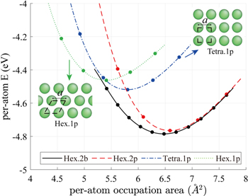
Figure 4. DFT-GGA calculation of the per-atom energy versus the per-atom occupation area (= area/number of atoms in the unit cell) in four different 2D Si structures: buckled (Hex.2b), planar (Hex.2p), rectangular (Tetra.1p), and hexagonal (Hex.1p). The Tetra.1p and Hex.1p structures are included in insets. For the Hex.2b and Hex.2p structures, readers are advised to refer to figure 1. The configurations in dots are sampled for potential parameter optimization.
Download figure:
Standard image High-resolution imageFor this purpose, the authors proposed the objective function fobj in equation (2), where X is an array of ten fitting parameters and thus a design variable in the optimization process.

The first term fA is a penalty term that was introduced to match the overall shape of the energy curves for all four structural types in MS as closely as possible to those obtained from DFT calculations.

where α ∈ {Hex.2b, Hex.2p, Tetra.1p, Hex.1p} and Nα is the number of sampled points (denoted as dots) from each curve in figure 4. We have sampled more points (Nα=Hex.2b = 11) from the Hex.2b curve (black solid line) than the other three because the Hex.2b structure is the most stable. In total, 26 configurations are sampled within a ±10% change of equilibrium lattice constant (a0) from four different types of structure for optimization. The energy difference ΔE in equation (4) is defined in equations (4) and (5).


where {x}α,m is the atomic configuration of the mth sampled point in the αth structural type and {x0} is the atomic configuration at the energy minimum point of the Hex.2b structure obtained from DFT. The second term fB is the correction term to shift the energy point evaluated at {x0} from MS to be as close as possible to the one in DFT (see equation (6)).

The optimal parameter set is searched by minimizing the objective function fobj with a constraint that the gradient of the interatomic potential energy would be zero at {x0} or  Since fobj has multiple local minima and is not a simple quadratic function of X, the search results are dependent on the parameters' initial value. Therefore, multiple initial sets X0 are produced by setting up a suitable grid in the design space. The preset range of each parameter is equally divided and combinations of initial parameters are made from each grid point. Minimizing fobj is done by the MATLAB command fmincon, which uses the interior-point algorithm for constrained nonlinear optimization [41, 42]. The number of maximum iterations is fixed at 106 and the criterion of the stopping residual is set to 10−6.
3.2. Parameter optimization results
Table 3 lists the optimized Tersoff parameters and their fitting range. With the optimized parameters, we evaluate buckled (Hex.2b) silicene to obtain the lattice constant of a = 3.7 Å, the buckling parameter Δ = 0.45 Å and the cohesive energy of 4.855 eV in table 1. It is unsurprising that our model outperforms the other potential models: EDIP [26], Tersoff [27], Murty and Atwater (MA95 [28], MA2013 [29]), Stillinger and Weber (SW92 [31], SW2014 [24]), MEAM [30], and ReaxFF [17] because the buckled structure at the energy-minimum point is included during optimization. Among the tested potentials, EDIP, Tersoff, and MA95 produce a planar (Hex.2p) structure as the most stable one in contrast to the DFT prediction and we exclude these three models from the subsequent benchmark test in section 4. Surprisingly, our parameter set predicts that not only Hex.2b but also Hex.2p, Tetra.1p and Hex.1p exist as metastable structures. This polytype feature is attributed to the bond-order nature of the Tersoff potential. Table 1 includes the lattice constants (a) and cohesive energies (Ec ) of Hex.2b, Tetra.1p, and Hex.1p as well.
Table 3. Optimized parameters and original Tersoff parameters listed for comparison.
| Parameters | Original [27] | This study | Fitting Range | |
|---|---|---|---|---|
| Min. | Max. | |||
| A | 1830.8 | 365438.7937887955 | 1e−6 | 1e+6 |
| B | 471.18 | 47.705032464589515 | 1e−6 | 1e+6 |
| λ1 | 2.4799 | 5.758230227112289 | 1e−6 | 1e+6 |
| λ2 | 1.7322 | 1.064947100817549 | 1e−6 | 1e+6 |
| λ3 | 1.7322 | 1.495435203249926 | 1e−6 | 3.0 |
| α | 0.0 | · | · | |
| β | 0.000001100 | 0.063800750093780 | 1e−6 | 1e+6 |
| n | 0.78734 | 1.000730918364174 | 1.0 | 3.0 |
| c | 100390 | 987179.8278956902 | 1e−6 | 1e+6 |
| d | 16.217 | 489.9549687344676 | 1e−6 | 1e+6 |
| h | −0.59825 | −0.441505852791745 | −0.5 | 0.0 |
| R | 3.0 | · | · | |
| D | 0.2 | · | · | |
| p0 | NA | 1.01750528410300 | −1e+6 | 1e+6 |
| p1 | NA | 1.12015635336776 | −1e+6 | 1e+6 |
| p2 | NA | 15.7996225229712 | −1e+6 | 1e+6 |
| p3 | NA | 19.2809433774420 | −1e+6 | 1e+6 |
| p4 | NA | −97.6602154288926 | −1e+6 | 1e+6 |
| h2 | NA | −0.473869564613929 | −0.5 | 0.0 |
The reference energy curves in figure 4 were reproduced with the optimized Tersoff model and plotted in figure 5. Figure 5(a) shows the energy curves of the buckled structure (Hex.2b) and planar structure (Hex.2p). The dashed curves are from the Tersoff model and they follow the trend of the DFT-GGA energy curves (solid lines) relatively well, although the entire curves are shifted downward by about 0.2 eV. A good factor of this parameter set is that the crossing between Hex.2b and Hex.2p energy curves is captured, which is crucial for predicting the structural change of silicene under extensional loading. Figure 5(b) compares the results of DFT-GGA and the optimized model for rectangular structure (Tetra.1p) and hexagonal structure (Hex.1p). Note that, contrary to the DFT-GGA results (solid lines), the hexagonal structure (Hex.1p) has lower energy than the rectangular structure (Tetra.1p) in the Tersoff model (dashed lines). While this opposite behavior initially looks disappointing, these two structures will not be observed in MD simulations in ambient conditions because both the Tetra.1p and Hex.1p structures have much higher energy than the buckled (Hex.2b) and planar (Hex.2p) structures. Therefore, we take the parameter set in table 3 as our best.
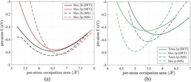
Figure 5. Per-atom energy curves of (a) buckled (Hex.2b) and planar (Hex.2p) structures and (b) rectangular (Tetra.1p) and hexagonal (Hex.1p) structures. Solid lines indicate the DFT calculation results and dashed lines indicate the Tersoff model with optimized parameters.
Download figure:
Standard image High-resolution image4. Benchmark
4.1. Elastic properties of silicene
As a benchmark test, we compared the elastic properties predicted from five different interatomic potential models (MA2013 [29], SW92 [31], SW2014 [24], MEAM [30], and ReaxFF [17]) together with ours. The crystal orientation of silicene used in MS was set to be the same as that used in DFT calculations (ZZ direction along the x axis and AC direction along the y axis). The initial structures were created using the conjugated-gradient (CG) method at 0 K. The tensile test along the ZZ direction used a silicene strip of 5120 atoms the area of which was about 32 nm × 11 nm. The test along the AC direction used a silicene strip of 4928 atoms the area of which was 30 nm × 11 nm. Periodic boundary conditions were applied in all directions and the simulation cell size in the silicene-plane normal direction was set to 8 nm, which was long enough to prevent image interaction. During the test, CG relaxation with the Parrinello–Rahman scheme was applied to release stress components except the tensile component and to find a minimum-energy structure at each strain increment. All MS simulations were performed using the Large-scale Atomic/Molecular Massively Parallel Simulator [43] and visualized with OVITO [44] and Atomeye [45]. Among the tested potentials, only ReaxFF and SW2014 were developed specifically for silicene. SW2014 was intended to better predict the phonon curve of silicene than the original SW (SW85 [46]). ReaxFF was developed to find the elastic constants and study the fracture pattern and edge reconstruction of silicene during uniaxial tensile tests.
In table 2, elastic constants (Y2D, ν, and B2D) from our model are compared with those from other models. All tested potentials predict the isotropic behavior of silicene. Y2D from our study is 59.8 (N m−1) in both the ZZ and AC directions and is closest to the reference DFT value (61.4 N m−1). The 2D bulk modulus B2D is 36 (N m−1), which is 80% of the reference value and still better than any other model. The Poisson ratio ν is 0.17, which is only 55% of the reference but reasonably fair, considering the others' performance. To better visualize the performance of our model at a glance, the authors present figure 6, which is a scatter plot of the elastic constants from the tested parameter sets in the (Y2D, B2D) plane. The point (in diamond red marker) from the optimized parameter set is closest to that of DFT-GGA marked with ×. This scatter plot shows that our model outperforms other potential models in that it better predicts silicene's elastic behavior overall.
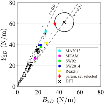
Figure 6. Scatter plot of elastic constants from trial parameter sets in the plane of (Y2D, B2D). The results from MS with different potential models and DFT are shown together for the purpose of comparison. Small black dots denote trial parameter sets and dashed grey lines are the border lines of the Poisson's ratio ν = 0 and ν = 0.31, which confine our search space. The chosen parameter set (the red diamond mark) is closest to the DFT result (marked with an ×) and outperforms the other existing potential models.
Download figure:
Standard image High-resolution image4.2. Tensile test in large deformation
The uniaxial tensile test was carried out quasi-statically with six potential models until ε ≤ 30%. Figures 7(a) and (b) show the stress and strain curves in the ZZ and AC directions, respectively. Our optimized model (red line) closely follows the DFT curve (black line) up to ε11 = 8.1% in the ZZ direction and about ε22 = 10% in the AC direction. All other potential models show much softer behavior across the entire strain range. In figure 7(a), our model starts to deviate at ε11 = 8.1% where the silicene structure changes from Hex.2b to Hex.2p, while DFT predicts that such a transformation occurs at ε11 = 21%. This early transformation is explained by the early crossing of the energy curves of Hex.2b and Hex.2p in our model in figure 5(a). Our model also shows a cusp in the stress curve at the transformation strain and abrupt stiffened behavior after the cusp, which was not observed from the DFT curve within our stress accuracy. As loading beyond the transformation strain (εT ) and unloading produce hysteresis in the stress curve, we can say that εT is the elastic limit. Interestingly, this stiffening after a structural change is universally observed from all tested interatomic potentials. The Hex.2b structure of SW92, MA2013, MEAM and ReaxFF transformed into Hex.2p at ε11 = 24.3%, 25.6%, 25.8% and 23.1%, respectively. Only the SW2014 model could predict a similar transformation strain of ε11 = 8.45% to our study. We speculate that the transformational stiffening is related to the higher elastic modulus of the planar silicene than that of the buckled, regardless of the tested potentials.
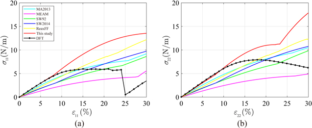
Figure 7. Stress–strain curves predicted from MS with different potential models and DFT in uniaxial tensile tests (a) along the ZZ direction and (b) along the AC direction.
Download figure:
Standard image High-resolution imageFigure 7(b) shows tensile tests along the AC direction that show how the Hex.2b structure is also altered into a Hex.2p structure for all potential models, while the DFT calculation predicts such transition at a much larger strain of ε22 = 40%. The dependency of structural transition strain (εT ) on the tensile loading direction implies the development of anisotropic behavior in silicene. Indeed, by comparing the stress curves between figures 7(a) and (b), it can be noted that the DFT results only show isotropic behavior in small strain regimes (<4%) but strong anisotropy for ε > 4% while no potential models can capture the appearance of anisotropy at this early stage of strain. The anisotropy is confirmed if σ11 and σ22 differ by more than 0.1 N m−1, which is approximately of the order of 0.1 GPa in 3D, a stress tolerance used in a DFT study of anisotropy in graphene [47]. Based on the same criteria, the anisotropy appears at ε = 6.4%, 12.4%, 7.1%, 6.8%, 11.5% and 7.1% for MA2013, MEAM, SW92, SW2014, ReaxFF, and our model, respectively. The authors expect that the puckered shape of the buckled structure causes the early development of anisotropy in silicene. This explanation is plausible if we compare silicene to graphene. Graphene, which is analogous to silicene but completely flat, maintains isotropic behavior until 15% strain according to DFT studies [47–49]. Although our optimized Tersoff model does not completely reproduce every feature reported in DFT calculations, it is the most reliable model so far, at least in the elastic regime.
5. Development of new angle penalty function
5.1. Modification of the angle penalty function
It is noticeable that a discontinuous slope increase appears in the stress–strain curve when the structure changes into Hex.2p in figure 7. This abrupt stiffening is associated with the geometric constraint that is inherent in the Hex.2p structure, where the sum of all three triplet angles between an atom and its three neighbor atoms must be 360°. That means that one angle (θ1) is dependent on the other (θ2)—as shown in inlet figure 8(a)—once the silicene becomes planar. To investigate the effect of angle function g(θ) on the potential energy, the per-atom energy depending on the triplet angle is calculated via DFT and the MS-Tersoff model with the optimized parameter set (see figure 8(a)). In this calculation, the interatomic distance is fixed at 2.278 Å, the bond length at the most stable configuration of Hex.2b. The difference between the results of DFT and MS becomes noticeable for θ > 130°. The energy increase is steeper in MS-Tersoff than DFT as θ increased, which can be attributed to the steep increase in the original angle penalty function g(θ) in the Tersoff model with the triplet angle (θ) in figure 8(b). We need a mildly increasing penalty function to better describe the angle effect.
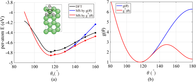
Figure 8. (a) Per-atom energy curves calculated with the original and new angle penalty functions g(θ) and g*(θ), compared with DFT. In the Hex.1b structure (θ1 < 120°), all three triplet angles change simultaneously (θ1 = θ2 = θ3). In the Hex.1p structure (θ1 ≥ 120°), all atoms are located on the same plane and the triplet angles are constrained with Σθi = 360° and θ2 = θ3. (b) Original and new angle penalty functions g(θ) and g*(θ).
Download figure:
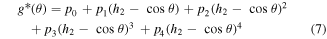
Standard image High-resolution imageA fourth-order polynomial function is selected as the new angle penalty function g*(θ) (equation (7)) that is padded to the original function after 120°. In other words, we use the original function g(θ) for θ ≤ 120° and the new function g*(θ) for θ > 120°. Thus, the elastic modulus of Hex.2b (θ = 116.2°) is unaffected by a new angle penalty function. Additional optimization of g*(θ) is conducted using the method described in section 3.1, with six parameters (p0, p1, p2, p3, p4, and h2). The reference configurations used in this second round of optimization are denoted as dots in figure 8(a), or α ∈ {Hex.2b, Hex.2p} in equations (4)–(6). Three nonlinear constraints in equations (8)–(10) are imposed during optimization to preserve C2 continuity at 120°, which is crucial for stress continuity.


5.2. Effects of the new angle penalty function
The lower part of table 3 summarizes the optimized parameters for g*(θ), which is plotted in figure 8(b) together with g(θ). With g*(θ), the per-atom energy curve clearly follows the trend of the DFT curve after 130° in figure 8(a). The constant shift between MS and DFT remains because we use the original function g(θ) for θ ≤ 120° and the per-atom energy curve must be continuous at θ = 120° even though it is not smooth. Uniaxial tensile tests were performed to calculate the elastic moduli and draw stress–strain curves to confirm the effect of g*(θ). The elastic moduli, including Y2D and ν, were maintained regardless of the direction, as intended. Figure 9 shows that the slope after transformation to the Hex.2p structure decreased in uniaxial tensile tests along both the ZZ and AC directions.

Figure 9. Stress–strain curves of the tensile tests with the original (g(θ)) and new angle penalty function (g*(θ)): (a) ZZ direction and (b) AC direction.
Download figure:
Standard image High-resolution image
6. Summary
In this study, mechanical tests of silicene were carried out using DFT and MS simulations. According to DFT, a uniaxial tensile test along the ZZ direction showed the structural change from buckled (Hex.2b) to planar (Hex.2p) and rectangular (Tetra.1p) structures, whereas in the AC direction structural change to planar occurred at a much larger strain of ε22 = 40%. Therefore, we expect that structural transformation under loading in the AC direction would be rarely observed at elevated temperatures or in the case of silicene with free boundary, both of which would promote structural failure at earlier strain. Silicene isotropically behaves in a small strain regime (ε < 4%) and becomes anisotropic. Based on the DFT results of biaxial stretch test for four metastable structures, including buckled (Hex.2b), planar (Hex.2p), rectangular (Tetra.1p), and hexagonal (Hex.1p), the Tersoff potential model was optimized using gradient-based minimization with a grid search in the hyperdimensional parameter space. As a result, the obtained optimized parameter set could predict better elastic behavior than other potential models tested in this study. The stress–strain curve predicted by the optimized Tersoff model was similar to that of DFT for εΤ ≤ 8.1% along the ZZ direction and εΤ ≤ 10% along the AC direction before structural change occurred. At the transformation strain (εΤ ), silicene changed its structure from buckled (Hex.2b) to planar (Hex.2p), where a cusp was observed in the stress–strain curve in our model. To suppress the steep slope after this cusp, the authors introduced a new angle penalty function that reduced the slope of the stress–strain curves to some degree. Interestingly, the cusp and steep slope after the cusp in the stress–strain curve were also observed in the MA2013, SW, MEAM, and ReaxFF potential models. Thus, similar problems exist in all potential models and this issue warrants further investigation. Although our optimized Tersoff model does not completely reproduce all features captured from DFT calculations, it has been the most reliable so far for describing the mechanical behavior of silicene over other models, at least until the transition strain.
Acknowledgments
This research was supported by the Basic Science Research Program through the National Research Foundation of Korea (NRF) funded by the Ministry of Education (2013R1A1A2063917, 2020R1A5A1019131), the Technology Innovation Program (Project No. 20012422, Development of lightweight materials superb mechanical properties based on AI) funded by the ministry of Trade, Industry and Energy, the Yonsei University Future-leading Research Initiative (2016-22-0106), and the Yonsei University Research Fund (Post Doc. Researcher Supporting Program) of 2020 (2020-12-0139).
Data availability statement
The data that support the findings of this study are available upon reasonable request from the authors.