
Abstract
Objective: Homeostasis is one of the key concepts of physiology and the basis to understand chronic-degenerative disease and human ageing, but is difficult to quantify in clinical practice. The variability of time series resulting from continuous and non-invasive physiological monitoring is conjectured to reflect the underlying homeostatic regulatory processes, but it is not clear why the variability of some variables such as heart rate gives a favourable health prognosis whereas the variability of other variables such as blood pressure implies an increased risk factor. The purpose of the present contribution is to quantify homeostasis using time-series analysis and to offer an explanation for the phenomenology of physiological time series. Approach: Within the context of network physiology, which focusses on the interactions between various variables at multiple scales of time and space, it may be understood that different physiological variables may play distinct roles in their respective regulatory mechanisms. In the present contribution, we distinguish between regulated variables, such as blood pressure or core temperature, and physiological responses, such as heart rate and skin temperature. Main results: We give evidence that in optimal conditions of youth and health the former are characterized by Gaussian statistics, low variability and represent the stability of the internal environment, whereas the latter are characterized by non-Gaussian distributions, large variability and reflect the adaptive capacity of the human body; in the adverse conditions of ageing and/or disease, adaptive capacity is lost and the variability of physiological responses is diminished, and as a consequence the stability of the internal environment is compromised and its variability increases. Significance: Time-series analysis allows one to quantify homeostasis in the optimal conditions of youth and health and the degradation of homeostasis or homeostenosis in the adverse conditions of ageing and/or disease, and may offer an alternative approach to diagnosis in clinical practice.
Export citation and abstract BibTeX RIS

Original content from this work may be used under the terms of the Creative Commons Attribution 3.0 licence. Any further distribution of this work must maintain attribution to the author(s) and the title of the work, journal citation and DOI.
1. Introduction
The term homeostasis attemps to convey two key ideas: (i) the internal stability of the human body, and (ii) coordinated adaptive responses in order to maintain this internal stability (Modell et al 2015). Physiology suggests that distinct types of variables are responsible for these two different aspects of homeostasis, where regulated variables such as blood pressure and core temperature are contained within a narrow range of values around a certain setpoint, whereas physiological responses such as heart rate and vasomotor action adapt to perturbations to ensure the stability of the former; see table 1. Homeostasis has become one of the key concepts to understand (patho)physiology, and the major regulatory mechanisms responsible for maintaining homeostasis have been identified: the sympathetic (SNS) and parasympathetic (PNS) branches of the autonomous nervous system (ANS), the endocrinological system and protective systems such as the the immune system and the integumentary system (Hall 2011). The simplest measures of homeostasis are point measurements of vital parameters, i.e. single measurements made at a specific moment in time, which can be compared with population-based normative ranges, and where deviations from these ranges may be an indication of disease (Hall 2011). These point-measurements and normative ranges, however, are the end-result of the homeostatic regulatory processes, which gives information on the stability of the internal environment, but do not provide insight into the dynamics or adaptive aspects of homeostasis. For this purpose, standardized clinical 'stress' tests have been developed where the patient is submitted to specific standardized challenges or stimuli to study the corresponding physiological responses. Non-adaptive responses, i.e. responses which are too strong, too weak, or which come too delayed in order to cope efficiently with the challenge, may be an indication for disease. Examples of such standardized clinical tests are cardiac exercise stress testing to investigate chronic heart disease (Pescatello et al 2014), Ewing's battery of autonomic reflex tests for neuropathy (Ewing et al 1985), and the glucose tolerance test for diagnosis of early-stage diabetes (Stumvoll et al 2000). However, these tests are time-consuming and intensive, both for the patients and for the treating clinician, and it may not be possible to perform these tests in vulnerable populations of weak patients or elderly adults, and these tests do not form part of a routine screening of the general population. On the other hand, recent technological advances allow one to monitor many different physiological variables in a non-invasive and continuous way, and the time evolution or time series of these variables is conjectured to reflect the dynamics of the underlying homeostatic regulatory mechanisms and to correlate with the health status of the organ, process or system under study (Seely and Macklem 2004). Most—if not all—of these variables spontaneously fluctuate in time, even when the monitored subject is in rest, possibly because the human body is always subjected to a wide variety of minor stimuli, which can come from the outside environment such as ambient temperature variations, and/or from the internal environment such as digestion, mental stress or internal reparation or restorative processes (Goldberger et al 1990). Intriguingly, for some variables a high variability is interpreted an indication of good health, as in the case of heart rate variability (HRV) (Malik et al 1996), whereas in other cases—on the contrary—it implies a risk factor, as in the case of blood pressure variability (BPV) (Parati et al 2013).
Table 1. Examples of homeostatic regulatory mechanisms where regulated variables are distinguishable because of their specific sensors and are maintained close to normative values by means of physiological responses which absorb or adapt to perturbations from the inner and outer environments. With permission on Modell et al (2015), Copyright 2015 by the American Physical Society.
| Examples of homeostatic regulatory mechanisms | |||
|---|---|---|---|
| Regulated variable | Physiological responses | ||
| Variable | Normative value | Sensor | No sensors nor normative values |
| Systolic blood pressure (BP) | 120 mmHg | Baroreceptor | Cardiac output (heart rate, stroke volume) |
| Vasomotor action (constriction, dilation) | |||
| Core temperature(Tc) | 37 °C | Thermoreceptor | Vasomotor action (constriction, dilation) |
| Skin temperature | |||
| Shivering, sudomotor | |||
| Blood oxygen saturation (SpO2) | 95% | Chemosensor | Respiration dynamics (rate, volume) |
| Blood glycemia | 10 mg dl−1 | Chemosensor | Insuline, glucagon |
The study of the variability of most physiological variables is at the level of basic research, and it is not at all clear how diverse physiological systems and organs coordinate their functions over broad ranges of space and time. The focus of the recently proposed field of network physiology is to better understand how homeostasis and its counterpart of homeostenosis emerge as different physiological states, optimal versus maladaptive, respectively, from the interaction between many different physiological variables, with as an objective to improve clinical diagnosis, prognosis and preventive medicine, and to better understand ageing and chronic-degenerative disease (Bashan et al 2012, Ivanov et al 2014, Bartsch et al 2015, Liu et al 2015, Ivanov et al 2016). In the present contribution, we will study time series of the simultaneous monitoring of various physiological variables, at different time scales, and subjected to either a dominant stimulus or a wide variety of stimuli. We will illustrate how in optimal conditions of youth and health the statistics of these time series reflects the different roles these variables play in the corresponding regulatory mechanisms, and how in adverse conditions of ageing or disease the alteration of these statistics indicates a degeneration of physiological regulation.
2. Physiological time series while subjected to a dominant stimulus
Figure 1 illustrates the effect of rest and physical exercise on cardiac and respiratory physiology in a healthy male young adult. Physical activity can be quantified at the level of individual movements using triaxial accelerometry, where the acceleration vector  is composed of contributions from the sagittal (X), lateral (Y) and vertical (Z) directions. The absence of physical activity during supine rest (
 g) is characterized by physiological time series with high moment-to-moment variability, both for heart rate (HR) and breathing rate (BR). For low-intensity activity (a < 0.2 g), such as leisure activities inside the house with repeated sitting down and standing up, heart rate variability (HRV) and breating rate variability (BRV) appear to be even higher than during supine rest. On the other hand, for high-intensity physical activity (a > 0.8 g), such as running in a treadmill, HR and BR increase proportional to the physical effort and HRV and BRV become minimal. After the exercise, average HR and BR gradually return to their basal levels and also their variability recuperates over time.
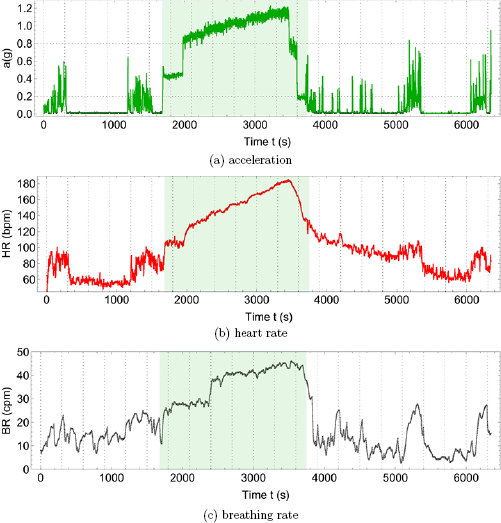
Figure 1. Effect of rest and physical exercise on cardiac and respiratory physiology in a healthy male young adult, (a) acceleration vector magnitude a in units of gravitational constant g = 9.81 m s−2, (b) heart rate (HR) in units of beats per minute (bpm), (c) breathing rate (BR) in unis of cycles per minute (cpm). Physical activity (shaded area) corresponds to warming up by walking on the treadmill for 5 min at 4 miles per hour (mph), running on a treadmill at increasing velocities of 5, 6, 7, 8 and 9 mph for 5 min each, and cooling down by walking at 4.5 and 2 mph for 2 min each. Resting or minimal-intensity physical activity intervals (non-shaded areas) before and after the exercise correspond to supine or seated rest ( g) or low-intensity activities inside the house (a < 0.2 g). All data were collected using a Zephyr Bioharness3® device and are shown for a sample rate of 1 Hz. Vertical gridlines at 5 min intervals. Horizontal gridlines at limiting values a = 0.2 g (walking) and a = 0.8 g (jogging) according to the Bioharness manual.
Download figure:
Standard image High-resolution imageFigure 2 shows the effect of the alternation of day and night on the physiology of the same male young adult of figure 1 during 7 days of continuous monitoring. Panel (a) shows an actigraphy (act) time series, which is an average measure based on accelerometry, such as in figure 1(a), but where the number of movements is counted per sample time interval or 'epoch', in the present case arbitrarily chosen as 1min. Simultaneous to the actigraphy time series, panel (b) shows the cardiovascular variables of heart rate (HR) and systolic blood pressure (BP), and panel (c) shows body temperature variables of skin temperature Ts and core temperature Tc. The dominant feature of these time series is the circadian rhythm, i.e. the degree by which these variables are modulated by the periodic 24 h day–night cycle. The standard way to study the circadian rhythm contained in a time series  with N data points, is so-called cosinor analysis (Fossion et al 2017) where a cosine function
  is fitted to the data in order to calculate the circadian parameters of the average or mesor M, amplitude A, period T and acrophase
  (time of day for which the circadian rhythm maximizes). As shown in table 2, all variables of figure 2 adapt to the day–night cycle with an oscillation
  min (24 h). The circadian cycle for act, HR, BP and Tc maximizes in the early afternoon, whereas the maximum for Ts is early during the night. The coefficient of determination R2 quantifies what fraction of the variance of the time series is explained by the model function
  . R2 is 50%–70% for BP and Tc, about 30% for HR and Ts and minimal for act, indicating that for the former variables the major part of the variance is due to the circadian rhythm, whereas for the latter variables there is additional variance that cannot be explained by the circadian rhythm.
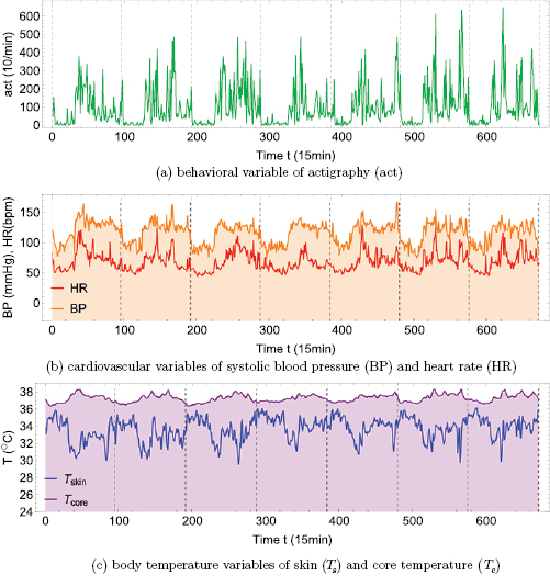
Figure 2. Seven day continuous and simultaneous monitoring of the healthy male young adult of figure 1 using (a) actigraphy in units of number of movements per minute (1/min), (b) cardiovascular variables of heart rate HR (bpm) and systolic blood pressure BP (mmHg), (c) body temperature variables of skin temperature Ts and core temperature Tc (°C). Curves of regulated variables (BP and Tc) have been shaded. Actigraphy was monitored with Actigraph wGT3X- , HR and BP with CONTEC ABPM50
 , and Ts and Tc with Maxim
  DS1922L iButtons ('thermochron8k'). All time series are shown for a sample rate of 1/15 min. Vertical gridlines at midnight.
Download figure:
Standard image High-resolution imageTable 2. Circadian parameters of average or mesor M (*), period T (min), amplitude A (*), acrophase  (in degrees ° or hours and minutes hh:mm after midnight) and coefficient of determination R2 for the 1 week time series of actigraphy (act), heart rate (HR), systolic blood pressure (BP), skin temperature (Ts) and core temperature (Tc) of figure 2. M and A are measured in the same units as the corresponding variable (*). See Fossion et al (2017) for technical details on the cosinor method used.
| Act (1/min) | HR (bpm) | BP (mmHg) | Ts (°C) | Tc (°C) | ||
|---|---|---|---|---|---|---|
| M | (*) | 964.68 | 67.96 | 115.78 | 33.57 | 37.12 |
| T | (min) | 1470 | 1470 | 1440 | 1425 | 1470 |
| A | (*) | 645.50 | 13.84 | 18.38 | 1.03 | 0.52 |
 |
 |
228.75 | 236.25 | 236.35 | 26.25 | 243.75 |
| (hh:mm) | 15:15 | 15:45 | 15:45 | 01:45 | 16:15 | |
| R2 | 0.160 | 0.387 | 0.518 | 0.295 | 0.693 |
3. Physiological time series while subjected to a wide variety of stimuli
3.1. Optimal conditions of youth and health
In order to compare the statistics of the fluctuations of each of the variables  of figure 2, dimensionless fluctuations
  can be defined around their respective average value
  and expressed as a percentage of this average value,

The behavior of these fluctuations can be illustrated using probability density functions (PDFs), which show the relative probability of a specific fluctuation  with respect to the range of fluctuations of the measured time series of that variable X, and where the area of each PDF has been normalized to 1 (unitary total probability). Figure 3 shows the PDFs of the fluctuations
  of the behavioral, cardiovascular and body temperature variables of figure 2, where positive values of
  indicate fluctuations above and where negative values of
  show fluctuations below the respective average
  . Variability of BP is small with respect to HR, variability of Tc is small with respect to Ts, and all physiological variables HR, BP, Ts and Tc are less variable than the behavioural variable act. The PDFs of BP and Tc correspond to the superposition of two Gaussians, with small fluctuations around two representative average values, which are the day and night setpoints. The PDFs of act, HR and Ts correspond to non-symmetric and skewed distributions with a broad maximum of small but frequent fluctuations at one extreme and a tail with large but less frequent fluctuations at the other extreme; comparison with the time series allows one to identify the broad maxima with night-time and the tail with day-time fluctuations.

Figure 3. Probability density functions (PDF) for dimensionless fluctuations  of variables of figure 2 according to equation (1) in linear scale for (a) actigraphy act, (b) cardiovascular variables of heart rate HR (red curve) and systolic blood pressure BP (orange curve), (c) body-temperature variables of skin temperature Ts (blue curve) and core temperature Tc (purple curve), and (d) comparison of PDFs of all variables in semilogarithmic scale. Curves of regulated variables (BP and Tc) have been shaded.
Download figure:
Standard image High-resolution image3.2. Adverse conditions of ageing and disease
We collected 5 min HR and BP time series in N = 30 control subjects, N = 30 asymptomatic subjects with recently diagnosed type-2 diabetes (DMA) and N = 15 long-standing patients with type-2 diabetes (DMB) in supine resting position, see Rivera et al (2016). Average age increases from the controls to the DMA and DMB groups because chronic-degenerative disease needs time to develop; see table 3. Exclusion criteria included smoking, cardiac arrhythmia, hypertension and having taken medication up to 48 h previous to the study. Examples of time series for individual subjects are shown in figure 4 (left-hand panels). Average heart rate  was similar for controls and the DMA group, but was significantly higher for the DMB group, whereas
  was comparable for the three groups. Figure 4 (right-hand panels) shows for each population the PDF for the fluctuations ΔHR and ΔBP, according to equation (1). For the control group, the distribution
  HR) is wider than
  BP), in particular, for ΔHR there is an asymmetric tail towards positive fluctuations up to 40% whereas ΔBP is constrained within the range
  to
to  . For the DMA group, the width of
  HR) is greatly reduced and in particular the positive ΔHR fluctuations have decreased below 30%, whereas now the probability distribution of ΔBP has become wider than that of ΔHR towards the negative side. For the DMB group, the situation is reversed with respect to the control group, where P(ΔBP) has become wider than
  HR), in particular, the positive ΔHR fluctuations are now limited to 20%, whereas the negative ΔBP fluctuations have increased up to 30%.
Table 3. Heart rate (HR) and systolic blood pressure (BP) for the control group, recently-diagnosed diabetic patient group (DMA) and the long-standing diabetic patient group (DMB) of figure 4. HR for DMB is significantly different from controls and DMA at the p = 0.05 level according to a Kruskal–Wallis test (*). Age and gender constitution of the three populations is also indicated.
| Control (N = 30) | DMA (N = 30) | DMB  |
|
|---|---|---|---|
| Gender | 17 females, 13 males | 16 females, 14 males | 10 females, 5 males |
| Age (years) |  |
 |
 |
| HR (bpm) |  |
 |
 (*) (*) |
| BP (mmHg) |  |
 |
 |

Figure 4. Time series for an individual subject of each group (left-hand panels) and average probability density functions (PDF) for populations (right-hand panels) of dimensionless fluctuations according to equation (1) for heart rate HR (red curves) and systolic blood pressure BP (orange curves) during 5 min of supine rest. Shown for (a) healthy control(s), (b) recently diagnosed diabetic patient(s) and (c) long-standing diabetic patient(s). HR is measured in beats per minute (bpm), BP in millimeters of mercury (mmHg), and time in units of beat number. Curves of regulated variable BP have been shaded. All data was collected using a  ®.Data from Rivera et al (2016). Figure based on Fossion et al (2018) © Springer International Publishing AG 2018. With permission of Springer.
Download figure:
Standard image High-resolution image4. Discussion
In section 2, the effect on physiology of a dominant stimulus is studied. High-intensity physical exercise on a treadmill, see figure 1, is an example of a continuous dominant stimulus, evoking a response of the sympathetic nervous system (SNS) which increases average heart rate  and breathing rate
  proportionally to the physical effort, in order to increase the oxygen supply to the muscles and the disposal of CO2 to the lungs (Hall 2011). Systolic blood pressure (BP) has also been reported to increase with exercise (Palatini 1988). The SNS decreases variability, as shown here for heart rate variability (HRV) and breathing rate variability (BRV), because the whole of physiology is focussed on the realization of one single task, and supply and disposal rates should be as constant and reliable as possible to maximize efficiency. The overall effect is not unlike a steam locomotive, the SNS being the train driver, where steam pressure and steam flow are increased in proportion to the desired speed. On the other hand, the parasympathetic nervous system (PNS) lowers HR, and temporal inhibition of the PNS induces episodes of HR accelerations, such that a modulation of the PNS is sufficient to take care of low-intensity leisure activities inside the house, and also internal processes such as digestion and restoration or reparation, and HRV is a reflection of the multitasking capabilities of the PNS. Measures of heart rate response to and heart rate recovery from a dominant stimulus are the basis for cardiac exercise stress testing (Pescatello et al 2014), and similar responses of various variables are used in other standardized clinical stress tests (Ewing et al 1985, Stumvoll et al 2000). On the other hand, circadian rhythms are an example of how physiological variables are modulated by the repetitive dominant stimulus of the 24 h day–night alternation, see figure 2, where the most obvious feature of the time series is a periodic behavior wich can be described approximately by a cosine function. The baseline value of physiological variables is reassigned according to a specific setpoint for day-time or night-time to allow a more efficient use of energy and resources, not unlike the different gears we use in bicycles or cars at different speeds. Loss of regularity of circadian rhythms may indicate underlying pathologies such as attention deficit hyperactivity disorder, age-associated frailty or insomnia (Fossion et al 2017). In hypertension, patients that display a nocturnal decrease in their BP profile ('dippers'), tend to have a more favourable clinical outcome than patients that do not exhibit circadian modulation ('non-dippers') or that have a nocturnal increase ('risers' or 'reverse dippers') (Mancia et al 2014). The conclusion of section 2 is that physiological variables tend to adapt to a dominant stimulus, and maladaptation to such a stimulus (responses that are too strong/weak or that arrive too early/late) may be an indication for adverse health conditions.
Section 3 discusses the effect on physiology of a wide variety of stimuli at ultradian time scales. Figure 3 suggests that some variables such as heart rate (HR) and skin temperature (Ts) tend to adapt to this wide variety of stimuli of various magnitude and time scales and therefore are characterized by a large variability, whereas other variables such as systolic blood pressure (BP) and core temperature (Tc) tend to remain approximately constant and close to a predetermined setpoint. The reason may be that for an organism it cannot be efficient to adapt as a whole to every single stimulus from its external environment, and a more optimal strategy would be to maintain some specific variables of the internal environment constant, so-called regulated variables, while absorbing as well as possible perturbations from the outer environment in the physiological responses of other so-called effector variables. Control theory and negative feedback loops indeed assign distinct roles to different variables, depending on their specific place in the control circuit, see figure 5, and also physiology and anatomy acknowledge that different variables may carry distinct responsabilities in homeostatic regulation; see table 1. The opposing statistics that we observed in figure 3, Gaussian distributions for regulated variables versus non-Gaussian, asymmetric and skewed distributions for physiological responses, reflects the complementary roles these variables play in the corresponding regulatory mechanisms in optimal conditions of youth and health. In the adverse conditions of ageing or chronic-degenerative disease, adaptive capacity of the physiological responses is increasingly lost which is reflected by a diminished variability of the associated time series, and as a consequence the stability of the internal environment is compromised and its variability increases. Figure 4 illustrates the adverse effects of type-2 diabetes mellitus on cardiovascular homeostasis, possibly aggravated as well by the aging process. Although by study design hypertensive patients were excluded such that no population differences could be observed for  , variability analysis reveals that adaptive capacity of HR decreases whereas the increase of temporary perturbations of BP indicates that homeostatic control is failing. In this way, we may understand intuitively the empirical observation in the literature that heart rate variability (HRV) is a protective factor for health Malik et al (1996), whereas blood pressure variability is a risk factor (Parati et al 2013).

Figure 5. Schematic homeostatic control loop with negative feedback. A regulated variable, e.g. systolic blood pressure (BP) or core temperature (Tc), is maintained within a narrow range around a pre-defined setpoint by the corrective action and physiological responses of associated effector variables, e.g. heart rate (HR) or skin temperature (Ts). Based on Modell et al (2015) Copyright 2018 by the American Physical Society.
Download figure:
Standard image High-resolution image
We argue that existing paradigms to explain the very rich phenomenology of the variability of time series have each focussed on either one of the two types of variables of table 1. On the one hand, the paradigm of early-warning signals of Scheffer (2009) and Carpenter et al (2011) discusses regulated variables of dynamic systems, which behave in a Gaussian way with low variability and little correlation or memory of past events while in a state of stability and equilibrium, whereas when the system approaches a critical threshold at the brink of collapse, statistical parameters such as variance, non-Gaussianity, correlations and memory tend to increase. The term 'early-warning' refers to the fact that countermeasures can be taken to avoid a catastrophe for dynamical systems such as the economy or the climate if these statistical fingerprints are detected early enough. On the other hand, the loss of complexity paradigm of Lipsitz and Goldberger (1992) discusses physiological responses, which are inherently 'complex' with a large variability that is increasingly lost with ageing and/or chronic-degenerative disease. West (2010) has suggested that these variables are characterized by heavy-tailed distributions such as power laws and that a new paradigm, fractal physiology, is needed to understand their behaviour. The fractal nature of physiological responses indicates that they are not white noise and that they behave according to specific correlations, although they do not obey any regulation that is hardwired into the feedback control loop as is the case of regulated variables. Therefore, one possibility is that they behave according to self-organized criticality, which operates in the vicinity of the critical point of a phase transition halfway between order and disorder (Bak 1996, Muñoz 2018), where physiological responses may strike an optimal balance between possibly opposite requirements from different corresponding regulated variables. For example, BP and Tc both depend on vasomotor action for their regulation, see table 1, such that vasomotor action might might self-organize in a critical point in the case of opposite requirements of BP and Tc. Table 4 makes an attempt to integrate the above paradigms of fractal physiology, early-warning signals and loss of complexity in a single scheme to explain the phenomenology of physiological time series. The present discussion is based on the pair-wise association of a regulated variable and a corresponding physiological response, e.g. blood pressure versus heart rate, or core temperature versus skin temperature, see table 1, where different homeostatic regulatory mechanisms are thought to be independent from each other. This approximation is of course not completely correct, because different regulation loops may be coupled by shared physiological responses (e.g. vasomotor action in the regulation of body temperature and blood pressure), and variables which are regulated at one time scale may play the role of physiological responses at another time scale (called nested homeostasis or hierarchy of homeostasis, see Carpenter (2004) and Modell et al (2015)), and a more general framework is needed to integrate these pair-wise relations into a more global network. The many new tools and methodologies offered by network physiology, including time delay stability (Bashan et al 2012, Ivanov et al 2014, Bartsch et al 2015, Liu et al 2015, Ivanov et al 2016), may explain how many different physiological variables from distinct homeostatic regulatory mechanisms interact together at many scales of time and space such that a physiological state of homeostasis emerges at the level of the organism.
Table 4. Scheme that incorporates various existing paradigms to interpret the phenomenology of physiological time series depending on their role in homeostatic regulation and depending on the type of stimulus they are subjected to.
| Dominant stimulus | Variety of stimuli | ||
|---|---|---|---|
| All variables | Regulated variables | Physiological responses | |
| Adaptability | Stability | Adaptability | |
| Optimal conditions (youth and health) | Normative response | Gaussian statistics | Fractal physiology (West 2010) |
| Self-organized criticality (Bak 1996, Muñoz 2018) | |||
| Adverse conditions (ageing or disease) | Non-normative response | Early-warning signals (Scheffer 2009, Carpenter et al 2011) | Loss of complexity (Lipsitz and Goldberger 1992) |
5. Conclusion
Technological advances allow one to monitor an ever increasing variety of physiological variables in a non-invasive and continuous way. It is not clear a priori how the time series of newly measured variables should behave statistically, or why a large variability of one variable represents a risk factor (e.g. blood pressure) whereas a large variability of another variable is an indication of health (e.g. heart rate). In the present contribution, we argue that the role a particular variable plays in the homeostatic control mechanism, a regulated variable versus an effector variable, determines the way the corresponding time series will behave statistically. With youth and health, a regulated variable such as blood pressure is maintained within a restricted homeostatic range with low variability, whereas effector variables and the corresponding physiological responses that adapt to perturbations from the inner and outer environment are characterized by a large variability. With ageing and/or chronic-degenerative disease, the capacity of these variables to play their respective roles is increasingly lost which is reflected by diminished statistical differences of the corresponding time series. We demonstrated these concepts for experimental data of heart rate and blood pressure for healthy controls and diabetic patients and we make the prediction that other pairs of regulated variables versus physiological responses, such as blood oxygen saturation versus respiration dynamics, or blood glycemia versus insulin and glucagon concentrations, should follow similar patterns. It will be up to the new field of network physiology to integrate these different pairwise relations of regulated variables versus physiological responses from distinct homeostatic regulatory mechanisms into a network in order to explain how homeostasis may emerge as a physiological state at the level of the organism.
Acknowledgments
Financial funding for this work was supplied by the Dirección General de Asuntos del Personal Académico (DGAPA) from the Universidad Nacional Autónoma de México (UNAM) with grants PAPIIT IV100116 and IA105017. We are also gratefully acknowledge grants 2015-02-1093, 2016-01-2277 and CB-2011-01-167441 from the Consejo Nacional de Ciencia y Tecnología (CONACyT). We are thankful for the Newton Advanced Fellowship awarded to RF by the Academy of Medical Sciences through the UK Government's Newton Fund program.