

Abstract
Objective: Interest in emotion recognition has increased in recent years as a useful tool for diagnosing psycho-neural illnesses. In this study, the auto-mutual and the cross-mutual information function, AMIF and CMIF respectively, are used for human emotion recognition. Approach: The AMIF technique was applied to heart rate variability (HRV) signals to study complex interdependencies, and the CMIF technique was considered to quantify the complex coupling between HRV and respiratory signals. Both algorithms were adapted to short-term RR time series. Traditional band pass filtering was applied to the RR series at low frequency (LF) and high frequency (HF) bands, and a respiration-based filter bandwidth was also investigated ( ). Both the AMIF and the CMIF algorithms were calculated with regard to different time scales as specific complexity measures. The ability of the parameters derived from the AMIF and the CMIF to discriminate emotions was evaluated on a database of video-induced emotion elicitation. Five elicited states i.e. relax (neutral), joy (positive valence), as well as fear, sadness and anger (negative valences) were considered. Main results: The results revealed that the AMIF applied to the RR time series filtered in the
  band was able to discriminate between the following: relax and joy and fear, joy and each negative valence conditions, and finally fear and sadness and anger, all with a statistical significance level p -value
  0.05, sensitivity, specificity and accuracy higher than 70% and area under the receiver operating characteristic curve index AUC
  0.70. Furthermore, the parameters derived from the AMIF and the CMIF allowed the low signal complexity presented during fear to be characterized in front of any of the studied elicited states. Significance: Based on these results, human emotion manifested in the HRV and respiratory signal responses could be characterized by means of the information-content complexity.
Export citation and abstract BibTeX RIS
1. Introduction
Interest in emotion recognition has burgeoned in recent years, aiming to provide a useful tool in the field of emotion regulation. In that sense, a subject's emotional response is mediated by individual influences depending on which emotions the subject has and how he/she experiences and expresses them (Gross 1998). Many clinical features of depression, stress, anxiety and mood disorders may be construed as maladaptive attempts to regulate unwanted emotions (Campbell-Sills and Barlow 2007). A system for emotion recognition could help people to manage their own emotions, providing a tool to record their feelings and consequently, focusing their attention on modulating their emotional responses.
A complex mixture of cognitive, affective, behavioral, and physiological factors contributes to individual differences in health and disease. All these factors produce wide variation in outcomes of heart rate variability (HRV), blood pressure and autonomic balance which have important implications for both physical and mental health (Thayer and Hansen 2009).
Human emotion recognition has been studied by means of HRV spectral analysis (Cohen et al 2000, Demaree and Everhart 2004, Bornasa et al 2005, Geisler et al 2010, Rantanen et al 2010, Quintana et al 2012, Mikuckas et al 2014, Valderas et al 2019). Generally, the power spectra of HRV is divided into two main components: low frequency (LF) component [0.04, 0.15] Hz, and high frequency (HF) component [0.15, 0.4] Hz (Task Force of ESC and NASPE 1996). This spectral HRV analysis can describe the regulatory mechanisms of the heart rate which are influenced by neural inputs from sympathetic and parasympathetic divisions of the autonomic nervous system (ANS), respiration, thermoregulation and hormonal systems, among others Task Force of ESC and NASPE (1996). The sympathetic modulation of cardiac activity is encompassed in LF band and the parasympathetic activity affects both LF and HF band power (Task Force of ESC and NASPE 1996). Furthermore, respiration has a dominant influence in the HF component of the HRV, since heart rate is increased during inspiration and reduced during expiration, phenomenon described as respiratory sinus arrhythmia (RSA) (Yasuma and Hayano 2004).
As before mentioned, HRV analysis based on linear methods (such spectral analysis) is a usual strategy for ANS analysis, although non-linear HRV analysis has also been demonstrated as a useful complementary tool (Hoyer et al 2002). Traditional time and frequency domain measures of HRV assess the amplitude of variations between subsequent intervals and the amplitude distributions in the power spectra, respectively. However, none of them provide information about the complex communication involved in the control of the cardiovascular system that generates the HRV (Palacios et al 2007). Non-linear techniques such as the dominant Lyapunov exponents, the detrended fluctuation analysis, the approximate entropy, the sample entropy, the fuzzy measure entropy, the cross sample entropy, the cross fuzzy measure entropy, the permutation entropy, permutation min-entropy, the pointwise correlation dimension, the lagged Poincaré plot or the quadratic coupling have been used to detect emotional stimuli and all of them have shown better results than linear techniques (Boettger et al 2008, Valenza et al 2012a, 2012b, 2012c, 2012d, 2014, Dimitriev et al 2016, Goshvarpour et al 2016, Xia et al 2018, Zhao et al 2019). Some of these techniques have also been used to study non-linear relationships between HRV and respiration signals (Valenza et al 2012b, 2012c, 2012d, Kontaxis et al 2019, Zhao et al 2019). Table 1 reports a summary of different non-linear techniques applied to RR series during diverse emotional states.
Table 1. Bibliographic summary of non-linear techniques applied to HRV series in different emotional states.
| Reference | Technique | Emotional state | Results |
|---|---|---|---|
| Valenza et al (2012a) | DLEs | Neutral and arousal elicitation | Mean ApEn decrease and DLEs became negative during arousal elicitation |
| ApEn | |||
| Boettger et al (2008) | AMIF | Depression | Increased total area under the AMIF curve are associated with major depression |
| Zhao et al (2019) | SEn | Depression | Increased CSEn and CFMEn are associated with depression severity |
| FMEn | |||
| CSEn | |||
| CFMEn | |||
| Xia et al (2018) | PE | Neutral, happiness, fear, sadness, anger, and disgust | Increased PE and PME during happiness, sadness, anger, and disgust |
| PME | PME is more sensitive than PE for discriminating non-neutral from neutral emotional states | ||
| Dimitriev et al (2016) | DLEs | Anxiety | Decreased DLEs, ApEn, SEn, PD2 and increased  during anxiety state during anxiety state |
| ApEn | |||
| SEn | |||
| PD2 | |||
| DFA | |||
| Goshvarpour et al (2016) | LPP | Peacefulness, happiness, fear, sadness | Maximum changes in LLP measures during happiness, and minimum changes during fear |
The nomenclature used are the following: Dominant Lyapunov exponents (DLEs), approximate entropy (ApEn). Sample entropy (SEn), Fuzzy measure entropy (FMEn). Cross sample entropy (CSEn), cross Fuzzy measure entropy (CFMEn). Permutation entropy (PE), permutation min-entropy (PME). Pointwise correlation dimension (PD2), detrended fluctuation analysis (DFA). Lagged Poincaré plot (LLP).
This complementary information can be assessed by non-linear methods such as the auto-mutual information function (AMIF) and the cross-mutual information function (CMIF), which have been demonstrated to be independent of signal amplitudes and able to describe the predictability and regularity of the signals (Hoyer et al 2002, 2006). Both functions, the AMIF and the CMIF, have been proposed as predictors of cardiac mortality (Hoyer et al 2002). The AMIF has been studied as an indicator of the increased cardiac mortality in depressed patients (Boettger et al 2008) and in multiple organ dysfunction syndrome patients (Hoyer et al 2006), and the CMIF has been applied to electroencephalographic signals for stress assessment (Alonso et al 2015).
In the present work, both the non-linear techniques, the AMIF and the CMIF are proposed for human emotion recognition. The AMIF technique is applied to HRV signals to study complex communication within the ANS, while the CMIF technique is considered to quantify the complex coupling between HRV and respiratory signals. Both algorithms are, in this work, adapted to short-term time series modifying the number of histogram bins involved in the methodology. Traditional RR band filtering is considered (i.e. LF and HF band), and also a redefined HF band ( ), centered at the respiratory frequency (FR) and whose width is determined based on the spectrum correlation HF (SCHF) method, are investigated (Valderas et al 2019). The aim of including the
  band is the analysis of RSA influences on HRV, mainly when FR is above 0.40 Hz or FR lies within the LF band (Bailón et al 2007, Valderas et al 2019). The ability of the parameters derived from the AMIF and the CMIF to discriminate elicited states is evaluated on a database of video-induced emotion elicitation, described in Valderas et al (2019).
In Valderas et al (2019), the discrimination between different emotional states was addressed using frequency domain HRV indices (linear features). However, it was not possible to discriminate between relax and all negative valences, as well as between fear and anger, and sadness and anger. Here, we aim to study the discrimination capability of the non-linear AMIF and CMIF techniques of emotions complementing the linear-feature information. We propose the use of these non-linear techniques for human emotion recognition hypothesizing that ANS response to different emotions will impinge differential regularity patterns in HRV and will change the complex interaction between respiration and heart rate variability.
2. Methods and materials
2.1. Data acquisition
A database of 25 healthy subjects was simultaneously recorded including electrocardiogram (ECG) and respiration signals during induced emotion experiments at University of Zaragoza Valderas et al (2019). The limb ECG leads (I, II and III) were sampled at 1 kHz and the respiration signal, r(t) at 125 Hz, with a MP100 BIOPAC Systems. The distribution of the subjects was: four men and five women for the age range 18–35 years, four men and four women for the age range 36–50 years and four men and four women over 50 years. All subjects were University students or employees with an estimated BMI of 22.9 kg m−2. Previous to the inclusion in the study, the adequacy of each user was evaluated with a general health questionnaire.
The experiment consisted on eliciting each subject by four emotions (joy, fear, anger and sadness) using videos (two videos per emotion). All the experiment extended over 2 consecutive days and two sessions were recorded each day. The experiment was split into two days, with the aim to have more than one sample per day for each emotion; therefore the recording is more representative of the emotion and not particularly biased for the specific mood of the day that was recorded. During sessions 1 and 4, the subject was stimulated with videos of joy (J) and fear (F), and during sessions 2 and 3 with videos of anger (A) and sadness (S). Therefore, each of the 25 subjects was elicited with two videos of the same emotion, resulting in a total of 50 recordings per emotion. All videos were presented in randomized order.
To ensure that the physiological parameters returned to the baseline condition, each video was preceded and followed by a relaxing video considered as baseline, which were excerpts from nature images with classical music. All sessions were recorded at the same time of the day and the order of the participant was maintained during all sessions to mitigate the circadian variations of HRV parameters. All videos were five minutes long, except a video corresponding to fear, which lasted three minutes. The video characteristics are presented in table 2.
Table 2. Specific video length and content.
| Video length (min) | Content | |
|---|---|---|
| Day 1: session 1 | ||
| Joy | 5 | Excerpts from laughing monologues |
| Fear | 3 | Excerpt from the scary movie 'Misery' |
| Day 1: session 2 | ||
| Sadness | 5 | Documentary film on war histories |
| Anger | 5 | Excerpt of the documentary film on Columbine High School massacre in 1999 |
| Day 2: session 3 | ||
| Sadness | 5 | Excerpt from the film 'the Passion of the Christ' |
| Anger | 5 | Documentary on domestic violence |
| Day 2: session 4 | ||
| Joy | 5 | Excerpts from laughing monologues |
| Fear | 5 | Excerpt from the scary movie 'Alien' |
All subjects in this experiment reported an agreement between the theoretical elicitation and the emotion felt. Additionally, the database was validated by 16 subjects, different from the ones participating in the experiment, using the positive and negative affect schedule—expanded form (PANAS-X) (Watson and Clark et al 1999). According to the analysis of the PANAS-X scale: joy emotion was identified as a positive valence of joviality, and fear, sadness and anger were verified as negative valences of fear, sadness and hostility, respectively.
Additional information of this database can be found in Valderas et al (2019). Institutional Ethical Review Boards approved all experimental procedures involving human beings, and subjects gave their written consent. The experiments were conducted following the protocol approved by the Aragón Research Agency under contract:  PM055, 2005.
2.2. Signal preprocessing
The RR interval was defined as the time between two consecutive R wave peaks, detected from the ECG lead with the best signal-to-noise ratio using a wavelet-based detector (Martínez et al 2004). The presence of ectopic beats and misdetections was detected and corrected (Mateo and Laguna et al 2003). Evenly sampled RR time series, RR(t), were obtained by linear interpolation at 4 Hz.
Then, the RR(t) was filtered in: (1) the LF band of [0.04, 0.15] Hz ( (t)), (2) the HF band of [0.15, 0.40] Hz (
 (t)) and (3) the
  band (Valderas et al 2019) based on the SCHF method, (
 (t)). In the SCHF method, the HF band was redefined to be centered at the FR and its limits were calculated by means of the cross-correlation function between the power spectrum of HRV and respiration, being subject-dependent. The maximum value of correlation determined the lower (
 ) and upper limit (
 ) of the
  band.
band.
The respiratory signal (r(t)) was filtered by a band pass filter from 0.04 Hz to 0.8 Hz, and downsampled at 4 Hz.
Then, a transformation of all time series was carried out by ranking data in order to have the best statistics in the entropy estimation and robustness against noise (Pompe 1998).
2.3. Auto-mutual information function
The AMIF is a non-linear equivalent of the auto-correlation function, based on the Shannon entropy. The Shannon entropy of a time series x(t) is calculated by the discrete probability distribution p (xi(t)) of x(t) leading Hx(t) as shown in equation (1) (Hoyer et al 2002):
where I is the number of bins needed for estimating the amplitude histogram of x(t), an approximation to the probability distribution function of the signal.
Then, the AMIF of x(t) is given by Hx(t), by  , obtained by shifting x(t) a time lag
  as x(
as x( ), and their bivariate probability distribution leading to
  as shown in equation (2) (Hoyer et al 2002):

Therefore, this function describes the amount of common information between the original time series x(t) and the time shifted time series x(t +  ). In the case of statistically independent time series, the
  is zero, otherwise positive. The AMIF is normalized to its maximum amplitude (in
  ) representing the entire information of a time series. The decay of this function over a time lag
  represents the loss of information with respect to this prediction time, and in the case of non-linear HRV analysis, it is assumed to quantify the complexity of autonomic communication (Hoyer et al 2006). In the case of a random and unpredictable time series, the AMIF decays to 0 for all prediction times
  apart from
  . On the contrary, in the case of a predictable time series the AMIF remains at 1 for all
  (Palacios et al 2007).
2.4. AMIF-based measures
In order to describe HRV complexity during emotion elicitation, the evolution of the information function over the time scale  should be taken into consideration. The AMIF (figure 1) applied to the RR(t) time series was characterized by the following parameters: BD is the beat decay that corresponds with the AMIF decay from
  s to
s to  s, which represents a standard mean beat period (Palacios et al 2007). Also,
  is the total area under the curve that has been proposed to characterize the morphology, predictability and regularity of the signal (Boettger et al 2008).
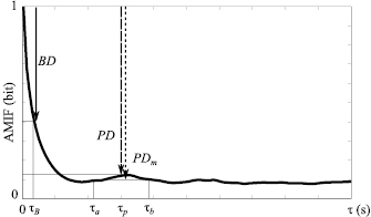
Figure 1. The normalized auto-mutual information function (AMIF) as function of the time scale  . The AMIF value at
  represents the entire information of a time series. Beat decay (BD) indicates the AMIF decay over a standard heart beat period (
 ). Mean peak decay (PDm) indicates the mean information decrease between
  and
and  . Peak decay (PD) indicates the information decay at the maximum peak (
 ) defined in the interval [
 ,
,  ].
].
Download figure:
Standard image High-resolution imageThe AMIF applied to the filtered time series  (t),
(t),  (t) and
  (t) was characterized by the following parameters:
  is the peak decay that shows the information decay at the maximum peak defined in the interval [
 ,
,  ];
];  is the mean peak decay within a time range [
 ,
,  ] that indicates the mean information decrease between two time lags
  and
and  ; and
; and  is the total area under the curve in the same time range [
 ,
,  ], where
  .
.
Since the information flow of oscillators has its peak starting at half the period  ), the lower and upper time scale boundaries [
 ,
,  ] within the AMIF were chosen at
  , where f is the frequency band boundaries used in the band pass filters (Hoyer et al 2006) as: (1) the traditional LF range of [0.04, 0.15] Hz corresponds to a LF prediction time range of
  = [
= [ ,
,  = 1/(2*0.04)] = [3.33, 12.5] s; (2) the traditional HF range corresponds to a HF prediction time range of [0.15, 0.40] Hz as
  = [
= [ = 1/(2*0.40),
  = 1/(2*0.15)] = [1.25, 3.33] s and (3) the SCHF band [
 ,
,  ] corresponds to a SCHF prediction time range of
  = [
= [ = 1/(2
 ),
),  = 1/(2
 )] s. In table 3, the values for lower- and upper-time scale boundaries corresponding to the SCHF prediction time range of
  in terms of median and interquartile ranges, as first and third quartile, (Median (Q1|Q3)) are specified.
Table 3. Median (Q1|Q3) values for lower- ( ) and upper-time (
 ) scale boundaries corresponding to the SCHF prediction time range for relax, joy, fear, sadness and anger.
| Elicitation |  |
 |
|---|---|---|
| Relax | 1.25 (1.19|1.43) | 2.38 (1.85|2.78) |
| Joy | 1.22 (0.98|1.28) | 2.00 (1.85|2.27) |
| Fear | 1.25 (1.14|1.39) | 2.08 (1.92|2.50) |
| Sadness | 1.25 (1.11|1.39) | 2.08 (1.85|2.50) |
| Anger | 1.25 (1.16|1.39) | 2.08 (1.85|2.38) |
2.5. Cross-mutual information function
The CMIF is a non-linear equivalent of the cross-correlation function, based on the Shannon entropy similarly to the AMIF, but quantifying the coupling between two signals x(t) and y (t). This function describes the amount of common information between a time series x(t) and a time shifted time series y ( ). Then, the CMIF of x(t) and y (t +
  ) is given by
  , by
, by  , and their bivariate probability distribution leading to
  as shown in equation (3) (Hoyer et al 2002):

In contrast to the AMIF, the CMIF is not normalized for its analysis and it does not present a symmetric distribution around zero. Therefore, left and right sides of the CMIF around zero were analysed. The non-linear analysis of the coupled signals using the CMIF was as described for the AMIF, i.e. the CMIF at  represents the common maximum information of both time series and the decay of this function over a prediction time describes the loss of information over this
  (Hoyer et al 2002).
2.6. CMIF-based measures
In order to quantify and extract the amount of mutual information between the synchronized registered time series of HRV and respiration during emotion elicitation, the coupling between RR(t) and r(t), and between  (t) and r(t) was investigated. Only the RR(t) and the
  (t) series have been taken into consideration because respiratory information is not consistently contained in the LF or HF bands for all subjects.
The following parameters were calculated from the CMIF of the synchronized cardiac and respiratory signals:  defined as the CMIF value at
  that represents the amount of common information between both time series without time lag;
  defined as the maximum CMIF value that shows the maximum coupling between the signals; and
  defined as the time lag between
  and
and  , that indicates the time lag between the amount of common information of the time series and the maximum coupling between the signals. For this analysis, the CMIF parameters were defined as follow:
  ,
,  and
and  in the coupling between each
  and r(t). In figure 2, it is presented a CMIF function.
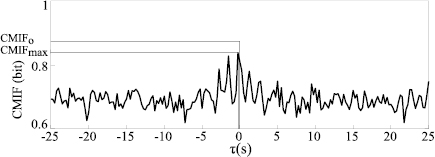
Figure 2. The CMIF of the coupling between RR(t) and r(t) as function of the time scale  . The CMIF value at
  = 0 (
= 0 ( ) represents the amount of common information of the time series without time lag and the maximum coupling between the signals is represented by
  .
.
Download figure:
Standard image High-resolution image2.7. Selection of the number of bins
The discrete probability distribution p(xi(t)) corresponds to a partitioning of the amplitude range of each signal in a histogram, and I = 2N represents the maximum possible information that can be obtained (I is the number of bins of the histogram and N is the number of bits).
In order to adapt the algorithms of the AMIF and the CMIF to short-term time series, 2N for N = {3, 4, 5, 6, 7, 8, 9} bits were considered in the calculation methodology. The number of parameters able to statistically discriminate between relax and emotions and between pairs of emotions were assessed to determine the adequate number of histogram bins I.
2.8. Statistical analysis
Normality distribution of all parameters was evaluated by Lillie test. Then, the T-test or the Wilcoxon test when necessary, depending on normality test results, was applied to evaluate differences for the followed paired conditions: relax and each emotion and also each emotion was compared with each other.
The significance statistical level was p -value  0.05, since this threshold provides a reliable value for statistical discrimination (Rice 1989). Additionally, the area under the receiver operating characteristic curve (AUC) was studied to analyse the capability of the parameters to discriminate the studied elicitations and AUC
  0.70 was used to determine statistically significant differences for each studied parameter. Furthermore, leave-one-out cross-validation method was used (Ney et al 1997) to assess sensitivity, specificity and accuracy values for each parameter in two-class emotion classification. These statistical parameters were required to be
  70% to determine statistically significant differences for each studied parameter. These thresholds have been selected as optimal cut-points values due to sensitivity and specificity being the closest to the value of the area under the ROC curve (Unal et al 2017).
The number of bins I was selected as the value which yielded the highest number of parameters with statistically significant differences (p -value  0.001) between relax and each emotion and between pairs of emotions.
3. Results
3.1. Selection of the number of bins
The following analyses have been performed to evaluate the adequate I for the AMIF and the CMIF calculation for emotion recognition using short-time HRV signals.
In figure 3, it is shown the percentage of the number of parameters that present statistically significant differences for each proposed I, when comparing relax with each emotions or between each pairs of emotions. The value I = 25 was selected, since it presents the highest number of parameters with statistically significant differences, p -value  0.001 and sensitivity, specificity and accuracy
  70% and AUC index
  0.70 for both non-linear techniques.
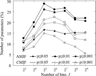
Figure 3. Percentage of number of parameters derived from the AMIF and the CMIF function of each proposed bin number I presenting statistically significant differences: (p -value  0.05, p -value
  0.01 and p -value
  0.001 when comparing relax and each emotion and between pairs of emotions. All these counted parameters also presented a sensitivity, specificity and accuracy
  70% and AUC index
  0.70).
Download figure:
Standard image High-resolution image3.2. AMIF-based measures
Those AMIF-based parameters that revealed statistically significant differences between relax and the different emotions or between pairs of emotions are presented in figure 4. In this figure, boxplots are shown in terms of median and interquartile ranges as first and third quartile:  (figure 4(a) for
  = {RR, LF, HF, SCHF}; BD (figure 4(b) analysed on RR(t); and
  (figure 4(c) for
  = {LF, HF, SCHF}.
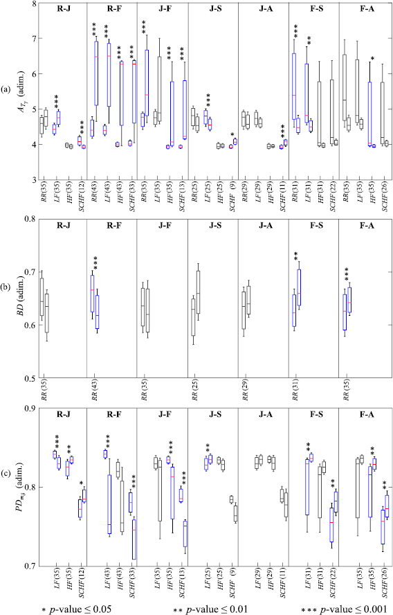
Figure 4. Boxplots of the parameters derived from the AMIF: (a)  for
for  = {RR, LF, HF, SCHF}; (b) BD analysed on RR(t); and (c)
  for
for  = {LF, HF, SCHF}. Only compared elicitations with some statistically significant differences are presented: relax and joy (R-J), relax and fear (R-F), joy and fear (J-F), joy and sadness (J-S), joy and anger (J-A), fear and sadness (F-S) and fear and anger (F-A). Statistical significance is denoted by * for p -value
  0.05, ** for p -value
  0.01 and *** for p -value
  0.001, all showed sensitivity, specificity and accuracy values
  70% and AUC index
  0.70. The number of the analysed subjects is indicated in parentheses.
Download figure:
Standard image High-resolution imageIn table 4, p -value, AUC and accuracy values are remarked in bold type for those AMIF-based parameters that revealed statistically significant differences between the emotional states studied. The presented emotion conditions were those which revealed statistically significant differences.
Table 4. Values of p -value, AUC and accuracy for the parameters derived from AMIF which statistically discriminate between some pair of elicitations: relax and joy (R-J), relax and fear (R-F), joy and fear (J-F), joy and sadness (J-S), joy and anger (J-A), fear and sadness (F-S) and fear and anger (F-A). The number of the analysed subjects for each parameter and pair of elicitations is indicated in parentheses.
| Parameters | R-J | R-F | J-F | J-S | J-A | F-S | F-A |
|---|---|---|---|---|---|---|---|
 |
(35) | (43) | (35) | (25) | (29) | (31) | (35) |
| p -value | n.s. |  0.001 0.001 |
 0.001 0.001 |
n.s. | n.s. |  0.001 0.001 |
 0.001 0.001 |
| AUC | 0.62 | 0.81 | 0.72 | 0.63 | 0.55 | 0.73 | 0.72 |
| Accuracy (%) | 61 | 77 | 71 | 64 | 60 | 73 | 73 |
 |
(35) | (43) | (35) | (25) | (29) | (31) | (35) |
| p -value |  0.001 0.001 |
 0.001 0.001 |
 0.05 0.05 |
 0.001 0.001 |
 0.05 0.05 |
 0.01 0.01 |
 0.05 0.05 |
| AUC | 0.76 | 0.82 | 0.64 | 0.71 | 0.62 | 0.73 | 0.67 |
| Accuracy (%) | 73 | 78 | 66 | 70 | 62 | 70 | 64 |
 |
(35) | (43) | (35) | (25) | (29) | (31) | (35) |
| p -value | n.s. |  0.001 0.001 |
 0.001 0.001 |
n.s. | n.s. |  0.001 0.001 |
 0.05 0.05 |
| AUC | 0.63 | 0.71 | 0.77 | 0.58 | 0.53 | 0.67 | 0.70 |
| Accuracy (%) | 64 | 70 | 71 | 62 | 57 | 65 | 70 |
 |
(12) | (33) | (13) | (9) | (11) | (22) | (26) |
| p -value |  0.001 0.001 |
 0.001 0.001 |
 0.001 0.001 |
 0.05 0.05 |
 0.001 0.001 |
 0.01 0.01 |
 0.05 0.05 |
| AUC | 0.83 | 0.75 | 0.95 | 0.88 | 0.85 | 0.66 | 0.68 |
| Accuracy (%) | 75 | 74 | 92 | 78 | 77 | 66 | 71 |
| BD | (35) | (43) | (35) | (25) | (29) | (31) | (35) |
| p -value |  0.01 0.01 |
 0.001 0.001 |
 0.01 0.01 |
 0.01 0.01 |
n.s. |  0.01 0.01 |
 0.001 0.001 |
| AUC | 0.65 | 0.78 | 0.68 | 0.67 | 0.62 | 0.72 | 0.71 |
| Accuracy (%) | 67 | 77 | 67 | 66 | 60 | 73 | 73 |
PD |
(35) | (43) | (35) | (25) | (29) | (31) | (35) |
| p -value |  0.001 0.001 |
 0.001 0.001 |
 0.01 0.01 |
 0.01 0.01 |
n.s. |  0.01 0.01 |
 0.05 0.05 |
| AUC | 0.76 | 0.81 | 0.63 | 0.71 | 0.61 | 0.70 | 0.67 |
| Accuracy (%) | 73 | 77 | 69 | 70 | 60 | 70 | 63 |
PD |
(35) | (43) | (35) | (25) | (29) | (31) | (35) |
| p -value |  0.01 0.01 |
 0.001 0.001 |
 0.001 0.001 |
n.s. | n.s. |  0.01 0.01 |
 0.01 0.01 |
| AUC | 0.70 | 0.71 | 0.81 | 0.64 | 0.59 | 0.68 | 0.72 |
| Accuracy (%) | 71 | 72 | 80 | 66 | 64 | 68 | 70 |
PD |
(12) | (33) | (13) | (9) | (11) | (22) | (26) |
| p -value |  0.05 0.05 |
 0.001 0.001 |
 0.001 0.001 |
n.s. | n.s. |  0.01 0.01 |
 0.01 0.01 |
| AUC | 0.72 | 0.81 | 0.99 | 0.79 | 0.64 | 0.74 | 0.70 |
| Accuracy (%) | 75 | 77 | 96 | 78 | 68 | 70 | 70 |
n.s. stands for non-significant.
aSensitivity or specificity  70%.
Note that parameters with p
70%.
Note that parameters with p  0.05, AUC index
  0.70, sensitivity, specificity, accuracy values
  70% are remarked in bold type.
3.3. CMIF-based measures
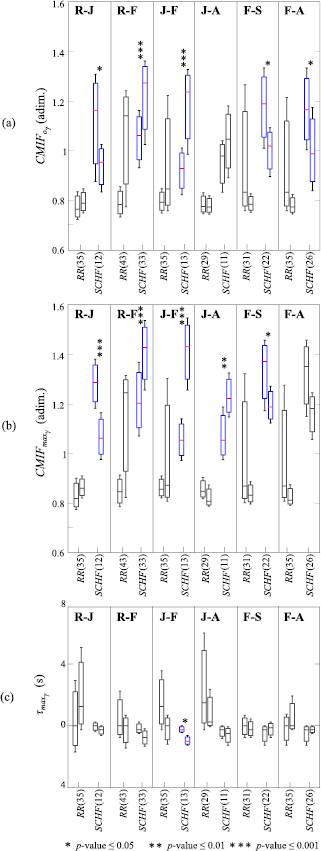
All parameters derived from the CMIF have been evaluated, however, only those that revealed statistically significant differences for their ability to discriminate between pair of emotions are shown in figure 5. In this figure, boxplots are shown in terms of median and interquartile ranges as first and third quartile:  (figure 5(a);
  (figure 5(b) and
  (figure 5(c) for the coupling between each signal
  = {RR, SCHF} and r(t).
Figure 5. Boxplots of the parameters derived from the CMIF: (a)  , (b)
, (b)  and (c)
  , for the coupling between each of the signals
  = {RR, SCHF} and r(t) and all emotion conditions studied with statistically significant differences: relax and joy (R-J), relax and fear (R-F), joy and fear (J-F), joy and anger (J-A), fear and sadness (F-S) and fear and anger (F-A). Statistical significance is denoted by: * for p -value
  0.05, ** for p -value
  0.01 and *** for p -value
  0.001, all with sensitivity, specificity and accuracy
  70% and AUC index
  0.70. In each x-axis the number of the analysed subjects is indicated in parentheses.
Download figure:
Standard image High-resolution image
In table 5, p -value, AUC and accuracy values are remarked in bold type for those CMIF-based parameters that revealed statistically significant differences between the emotional states studied. The presented elicited conditions were those which revealed statistically significant differences.
Table 5. Values of p -value, AUC and accuracy for the parameters derived from CMIF which statistically discriminate between some pair of elicitations: relax and joy (R-J), relax and fear (R-F), joy and fear (J-F), joy and anger (J-A), fear and sadness (F-S) and fear and anger (F-A). The number of the analysed subjects for each parameter and pair of elicitations is indicated in parentheses.
| Parameters | R-J | R-F | J-F | J-A | F-S | F-A |
|---|---|---|---|---|---|---|
 |
(35) | (43) | (35) | (29) | (31) | (35) |
| p -value | n.s. |  0.001 0.001 |
 0.01 0.01 |
n.s. |  0.01 0.01 |
 0.05 0.05 |
| AUC | 0.61 | 0.75 | 0.65 | 0.53 | 0.65 | 0.65 |
| Accuracy (%) | 61 | 78 | 70 | 53 | 66 | 64 |
 |
(12) | (33) | (13) | (11) | (22) | (26) |
| p -value |  0.05 0.05 |
 0.001 0.001 |
 0.001 0.001 |
n.s. |  0.05 0.05 |
 0.05 0.05 |
| AUC | 0.70 | 0.73 | 0.85 | 0.69 | 0.72 | 0.70 |
| Accuracy (%) | 71 | 73 | 85 | 64 | 70 | 70 |
 |
(35) | (43) | (35) | (29) | (31) | (35) |
| p -value | n.s. |  0.001 0.001 |
 0.05 0.05 |
n.s. |  0.01 0.01 |
n.s. |
| AUC | 0.62 | 0.72 | 0.60 | 0.64 | 0.63 | 0.66 |
| Accuracy (%) | 64 | 76 | 70 | 66 | 68 | 63 |
 |
(12) | (33) | (13) | (11) | (22) | (26) |
| p -value |  0.001 0.001 |
 0.001 0.001 |
 0.001 0.001 |
 0.01 0.01 |
 0.01 0.01 |
 0.01 0.01 |
| AUC | 0.88 | 0.74 | 0.95 | 0.79 | 0.77 | 0.68 |
| Accuracy (%) | 83 | 71 | 85 | 77 | 75 | 69 |
 |
(35) | (43) | (35) | (29) | (31) | (35) |
| p -value | n.s. | n.s. | n.s. | n.s. | n.s. | n.s. |
| AUC | 0.62 | 0.53 | 0.66 | 0.56 | 0.53 | 0.55 |
| Accuracy (%) | 66 | 55 | 67 | 57 | 56 | 57 |
 |
(12) | (33) | (13) | (11) | (22) | (26) |
| p -value | n.s. |  0.01 0.01 |
 0.05 0.05 |
n.s. |  0.05 0.05 |
n.s. |
| AUC | 0.62 | 0.68 | 0.75 | 0.66 | 0.62 | 0.51 |
| Accuracy (%) | 63 | 65 | 77 | 68 | 61 | 60 |
n.s. stands for non-significant.
aSensitivity or specificity  70%.
Note that parameters with p
70%.
Note that parameters with p  0.05, AUC index
  0.70, sensitivity, specificity, accuracy values
  70% are remarked in bold type.
4. Discussion
The AMIF and the CMIF techniques have been proposed to study the non-linear relationships between HRV and respiration for human emotion recognition. Both non-linear techniques may provide complementary information to that captured by linear techniques for emotion recognition.
The adequate number of bins I was estimated to adapt the AMIF and the CMIF algorithms to short-time signals for emotion recognition, since the values of I applied to long-term HRV may not be suitable for short-term. The value of I determines the histogram partitioning. The greater the I value is, the histogram represents more faithfully the probability density function. Nevertheless, each partitioning of the histogram needs to contain a minimum number of samples in order to capture the regularity and complexity signal contain more appropriately. Therefore, a compromise between the greatest number of partitioning of the histogram for faithfully describing the signal, and the adequate number of samples contained in each partitioning, should be taken into consideration.
In Hoyer et al (2002), the AMIF and the CMIF histogram were constructed by using 25 bins, when studying short-term RR signals according to Task Force guidelines (Task Force of ESC and NASPE 1996, Sassi et al 2015), in a group of patients after acute myocardial infarction and a control group. However, 23 bins were proposed in Hoyer et al (2006) for the AMIF histogram computation for short and long-term signals, to analyse the risk stratification of patients with multiple organ dysfunction syndrome, cardiac arrest patients and a control group. In this work, the highest percentage of number of parameters that presents statistically significant differences (p -value  0.001) between each pair of elicited states was obtained for I = 25 bins (see figure 3).
Table 6 displays the parameters which statistically discriminate between each pair of elicitations. The pair of elicited conditions which did not show statistically significant differences by means of any of the parameters considered in this work were: relax and sadness (R-S), relax and anger (R-A) and sadness and anger (S-A).
Table 6. Parameters derived from the AMIF and the CMIF which statistically discriminate between the studied elicitations.
| Compared elicited states | R-J | R-F | J-F | J-S | J-A | F-S | F-A |
|---|---|---|---|---|---|---|---|
| Parameters derived from the AMIF | |||||||
 |
— | Yes | Yes | — | — | Yes | — |
 |
Yes | Yes | — | Yes | — | Yes | — |
 |
— | Yes | Yes | — | — | — | Yes |
 |
Yes | Yes | Yes | Yes | Yes | — | — |
| BD | — | Yes | — | — | — | Yes | Yes |
PD |
Yes | Yes | — | Yes | — | Yes | — |
PD |
Yes | — | Yes | — | — | — | Yes |
PD |
Yes | Yes | Yes | — | — | Yes | Yes |
| Parameters derived from the CMIF | |||||||
 |
Yes | Yes | Yes | — | — | Yes | Yes |
 |
Yes | Yes | Yes | — | Yes | Yes | — |
 |
— | — | Yes | — | — | — | — |
The nomenclature used for the elicited states are the following: relax (R), joy (J), fear (F), sadness (S) and anger (A).
It should be noted that no statistically significant differences between relax and emotions or between pairs of emotions were found by any parameter derived from analysis of the coupling between the signals RR(t) and r(t). As it was found by analysing the AMIF technique, the pair of elicitation conditions which did not show statistically significant differences in the CMIF by means of any of the parameters considered was: relax and sadness (R-S), relax and anger (R-A), joy and sadness (J-S) and sadness and anger (S-A).
Regarding the ability of the AMIF parameters to discriminate emotions, the total areas (figure 4(a),  was the only parameter capable of statistically distinguishing joy and anger among all the studied parameters derived from the AMIF. This result shows the importance of redefining the boundary of the HF band for a correct evaluation of physiological changes of the ANS (Goren et al 2006, Valderas et al 2019). Fear revealed a greater median value than any other emotion. Note that an enlargement of the area under the AMIF curve indicates a better predictability of future heart beats, and therefore, a lower complexity (Boettger et al 2008).
Evaluating the beat decay BD (figure 4(b), fear presented smaller median values than any other compared elicitation. Furthermore, this parameter was able to statistically distinguish between fear and relax, sadness and anger. However, the remaining pair of compared elicited states did not show such a clear pattern as fear. Additionally,  (figure 4(c) presented a similar tendency as the BD for fear with a smaller median value than any other elicitation state. The BD and
  presented results with complementary information, and statistically significant values, and also adequate sensitivity, specificity, accuracy and AUC index.
The CMIF has been proposed to reveal non-linear cardiorespiratory interdependencies (Hoyer et al 2002), which might be altered during emotion elicitation. For example, a significant increase in the CMIF of electroencephalographic signals has been also observed in the presence of stress (Alonso et al 2015). In our study, the parameter  (figure 5(a) and the parameter
  (figure 5(b) provide similar information, although the slight differences in the calculation of both parameter revealed that
  is able to discriminate with an equal or better p -value, sensitivity, specificity, accuracy and AUC index than
  in all compared elicited states, except for fear and anger. Moreover, evaluating
  and
and  , it is possible to extract a similar pattern for fear presenting a greater median value than any other elicited state.
The time lag between  and
and  in the SCHF band was the only parameter able to distinguish between joy and fear, and it suggested less non-linear correlation between HRV and respiration during joy. A complexity reduction is observed during fear elicitation as reflected by a lower value of parameter
  .
.
Furthermore, joy or fear versus sadness can be discriminated by parameters obtained from  (t) signals and joy or fear versus anger from RRHF(t) signals. Predominant autonomic rhythms can be assessed by the complex information loss over their respective prediction time horizon (Hoyer et al 2002). In this sense, those parameters studied in the LF band reflect the complexity of vagal and sympathetic mechanisms, and those parameters studied in the HF band reflect the complexity of vagal and respiratory rhythms (Hoyer et al 2002).
Comparing the results obtained from the AMIF and the CMIF techniques, it is worth noting that filtering the HRV signals into a redefined HF band presents better discrimination power for parameters derived from the AMIF than from the CMIF ones. Furthermore, applying the CMIF into the RR time series filtered into the redefined HF band provided relevant complexity information to discriminate between HRV and respiratory mechanisms in the case of fear.
A complexity reduction is observed during fear elicitation as reflected by smaller BD, PD and
and  values together with a greater total area,
  and
and  .
.
In Bolea et al (2014), a physiological explanation of non-linear HRV parameters was reported. In this work, non-linear HRV indices during ANS pharmacological blockade and body position changes were studied in order to assess their relation with sympathetic and parasympathetic activities. Parasympathetic blockade caused a significant decrease in complexity values, while sympathetic blockade produced a significant increase in the non-linear parameters. We hypothesize that the decrease in complexity observed during fear elicitation reflects vagal activity, while more random RR series during joy might reflect sympathetic activity.
The results derived from this work have been compared with a previous work on the same emotion database, where a linear-based methodology was applied (Valderas et al 2019) (table 7). In both cases the HF band was analysed after redefining it considering the HRV-respiration interaction (Valderas et al 2019). All the elicited states able to be discriminated with linear techniques, remain discriminated with the non-linear features (table 7). In addition, during fear elicitation, heart rate presents a better predictability, implying lower complexity, as compared to other elicited states, resulting in extra discriminating power between fear and relax or anger (table 7) non accessible from linear features. These results may indicate that the non-linear indexes are suitable for discrimination between different emotions.
Table 7. Discriminating possibility in comparing between elicited states with linear and non-linear techniques.
| Compared elicited states | Linear techniques (Valderas et al 2019) | Non-linear techniques (this work) |
|---|---|---|
| R-J | Yes | Yes |
| R-F | No | Yes |
| R-S | No | No |
| R-A | No | No |
| J-F | Yes | Yes |
| J-S | Yes | Yes |
| J-A | Yes | Yes |
| F-S | Yes | Yes |
| F-A | No | Yes |
| S-A | No | No |
The nomenclature used for the elicited states are the following: relax (R), joy (J), fear (F), sadness (S) and anger (A).
Furthermore, other non-linear HRV parameters as the correlation dimension, the approximate entropy and the sample entropy have been investigated in the same emotional database. However, these parameters did not present the ability to separate the emotional states in this analysed database. In table 1, there are summarized the non-linear techniques used to detect emotional stimuli based on HRV analysis. In Valenza et al (2012a), the emotional states were conceptualized in two dimensions by the terms of valence and arousal. The dominant Lyapunov exponent and the approximate entropy techniques showed differences between the neutral and the arousal elicitation. These results are in concordance with the ones obtained in this study by means of the AMIF and the CMIF techniques, since statistically significant differences between the neutral state of relax and the two high arousal elicitations of joy and fear were found. Furthermore, it was found in Valenza et al (2012a) that the dominant Lyapunov exponent became negative, and the mean approximate entropy decreased during arousal elicitation. In accordance with the dominant Lyapunov exponent and the approximate Entropy, during fear elicitation the non-linear HRV parameters obtained in the present study revealed a reduced complexity level. In Boettger et al (2008), an increment of the total area under the AMIF curve was observed revealing an indication of decreased complexity of cardiac regulation in depressed patients. However, in Zhao et al (2019), a consistent increasing trend among most entropy measures for different depression levels was found. This suggested a reduced regularity and predictability of the depressed patients. The depression state is considered by means of the circumplex model of affect as having negative valence with low arousal, as can be sadness (Valenza et al 2012a). Considering the parameter  in the comparison between fear and sadness (emotional states with the same negative valence but different arousal), it could be observed that sadness presents a lower median value, being an indicator of decreased complexity as reported in Boettger et al (2008), and being in agreement with the results obtained by Zhao et al (2019). In Xia et al (2018), a significantly increase of the entropy measures was found during the emotional states of happiness, sadness, anger, and disgust. These results are in concordance with the ones obtained in this study for fear, which revealed increased regularity and a reduced unpredictability. In Dimitriev et al (2016), significant decreases in the entropy, the dominant Lyapunov exponent, and the pointwise correlation dimension, and an increase in the short-term fractal-like scaling exponent of the detrended fluctuation analysis were found during anxiety situations, compared with the rest period. These results suggest that an increase of anxiety was related to the decrease in the complexity. The anxiety state can be considered by means of the circumplex model of affect (Valenza et al 2012a) as having negative valence with high arousal, similar to fear. Both the state of anxiety studied in Dimitriev et al (2016) and the emotional state of fear, studied in this work, presented the same tendency in level of complexity. In Goshvarpour et al (2016), maximum changes in the lagged Poincaré Plot measures were found during the happiness stimuli, and minimum changes were obtained during the fear inducements. These results are in agreement with the ones obtained by means the CMIF technique applied in the present study, were differences between joy and fear could be found.
There are also some limitations to note regarding this study. First, the sample size database used is small. Nonetheless, the results obtained advocated in support of using the proposed approaches, although a bigger sample size database could probably yield better statistics. Second, likewise, long-time emotional monitoring could probably provide additional information that cannot be detected in short-time series analyses. Although, short-term emotional analyses are more suitable for outpatient patient monitoring and applications where the result is urgently needed. Third, there are emotions that could not be expressed by the subject all the time the videos last, but they have been treated as if the subject expresses that emotion all the time.
Despite these limitations, the parameters derived from the AMIF and the CMIF techniques which presented statistically significant differences for emotion discrimination seem to be good candidates to be implemented on a biomedical equipment, providing a tool for mental illness diagnoses. In addition, analysing the role of mutual information-based HRV measures to explore a multi-variable approach combining with other non-linear parameters could open a door to extract new suitable parameters for emotion recognition.
5. Conclusions
The results of this study suggested that the non-linear AMIF and the CMIF techniques characterized the negative valence of fear, by reflecting a lower complexity than the other emotions. Parameters derived from the AMIF allowed extending the description of the complexity of vagal and sympathetic autonomic rhythms. Parameters derived from the CMIF at the respiration-based bandwidth provided relevant information related to non-linear mechanisms between vagal and respiratory activity, especially for fear.
Furthermore, filtering the HRV signals into a redefined HF band provided a better discrimination for parameters derived from the AMIF between relax and joy, relax and fear, joy and all remaining emotion conditions as well as fear and all remaining emotion conditions.
The non-linear AMIF and CMIF techniques provided complementary information to other linear and non-linear methods.
Acknowledgment
Research supported by AEI and FEDER; under the projects RTI2018-097723-B-I00, DPI2016-75458-R and DPI2017-89827-R, by CIBER de Bioingeniería, Biomateriales y Nanomedicina through Instituto de Salud Carlos III, by LMP44-18 and BSICoS group (T39-17R) funded by Gobierno de Aragón. The computation was performed by the ICTS 'NANBIOSIS', more specifically by the High Performance Computing Unit of the CIBER in Bioengineering, Biomaterials & Nanomedicne (CIBERBBN).
Conflict of interest statement
The authors declare that the research was conducted in the absence of any commercial or financial relationships that could be construed as a potential conflict of interest.