
Abstract
The complex interaction of the magnetic field with matter is the key to some of the most puzzling observed phenomena at multiple scales across the Universe, from tokamak plasma confinement experiments in the laboratory to the filamentary structure of the interstellar medium. A major astrophysical puzzle is the phenomenon of coronal heating, upon which the most external layer of the solar atmosphere, the corona, is sustained at multi-million degree temperatures on average. However, the corona also conceals a cooling problem. Indeed, recent observations indicate that, even more mysteriously, like snowflakes in the oven, the corona hosts large amounts of cool material termed coronal rain, hundreds of times colder and denser, that constitute the seed of the famous prominences. Numerical simulations have shown that this cold material does not stem from the inefficiency of coronal heating mechanisms, but results from the specific spatio-temporal properties of these. As such, a large fraction of coronal loops, the basic constituents of the solar corona, are suspected to be in a state of thermal non-equilibrium (TNE), characterised by heating (evaporation) and cooling (condensation) cycles whose telltale observational signatures are long-period intensity pulsations in hot lines and thermal instability-driven coronal rain in cool lines, both now ubiquitously observed. In this paper, we review this yet largely unexplored strong connection between the observed properties of hot and cool material in TNE and instability and the underlying coronal heating mechanisms. Focus is set on the long-observed coronal rain, for which significant research already exists, contrary to the recently discovered long-period intensity pulsations. We further identify the outstanding open questions in what constitutes a new, rapidly growing field of solar physics.
Export citation and abstract BibTeX RIS

Original content from this work may be used under the terms of the Creative Commons Attribution 3.0 licence. Any further distribution of this work must maintain attribution to the author(s) and the title of the work, journal citation and DOI.
1. Introduction
The solar corona hosts several unsolved astrophysical mysteries. This outer layer of the solar atmosphere is characterised by being hot and tenuous, with average temperatures of a few million Kelvin, hundreds of times higher than the underlying photosphere (the solar surface), in what constitutes the famous coronal heating problem [1, 2]. The corona is highly structured and dynamic. It is mostly composed of magnetic loop bundles anchored in the photosphere, termed coronal loops. These structures become visible when filled with ionised plasma that is energised in unknown ways by the magnetic field, which itself is constantly stressed by magneto-convection below the photosphere.
However, not everything in the solar corona is hot. Perhaps even more mysteriously, like snowflakes in the oven, the corona hosts cool (≈104 K) and dense ( ) structures. Prominences, as their name suggest, are notoriously famous and a prime example of such cool material. These huge, filamentary and dense structures can remain for days or weeks suspended by the magnetic field in the high corona, in cycles of continuous evacuation and refilling [3–5], with mass circulation for a single prominence on the same order as for the entire corona. These massive structures often erupt, accompanied by a solar flare—among the most intense displays of energy release observed in stars—with a myriad of space weather effects at Earth. Another example of cool material in the solar corona, related to prominences but far more ubiquitous, is coronal rain (see figure 1).
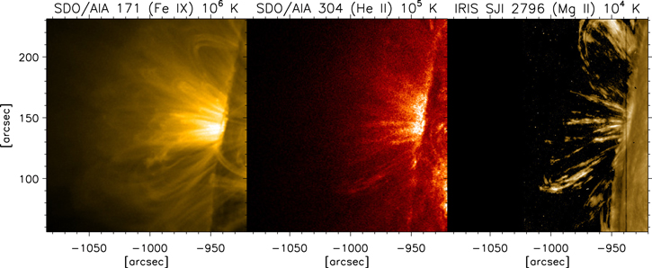
Figure 1. An active region at the East limb of the Sun on 2 June 2017, co-observed by SDO/AIA in the 171 (left panel) and 304 channels (middle panel), and IRIS SJI in the 2796 channel (right panel). The AIA 171 channel is dominated by Fe IX 171.073 Å emission, formed at  . The AIA 304 channel is dominated at cool temperatures by He II 303.78 Å formed at
  (at hot temperatures it has significant contribution from the Si XI 303.32 Å line, formed at
  ). The SJI 2796 channel is dominated by the Mg II k line, formed at
  . Coronal rain corresponds to the clumpy material seen in AIA 304 and SJI 2796 following the coronal loop structure as it falls down towards the solar surface.
Download figure:
Standard image High-resolution imageCoronal rain is probably the phenomenon most often used for public outreach purposes due to its spectacular characteristics. The most prominent example of coronal rain is that produced during a solar flare, where the solar atmospheric response to the large amount of heating from the flare comes in the form of a large and prolonged cooling in the form of coronal rain. However, this phenomenon is also one of the least understood in solar physics. Although observed for more than half a century (as shown by NCAAR archives), coronal rain has for a long time been considered as a rather sporadic phenomenon with minor importance in solar physics. The lack of a review article to date devoted to the subject is a clear reflection of this. It is only with the advent of high resolution multi-wavelength instrumentation in the last 10 years that the importance of coronal rain is now starting to transpire, being strongly linked to several of the big outstanding questions, not only in solar but also in stellar and interstellar physics. It is now fair to say that coronal rain constitutes a field of its own spawning a new, active research community in astrophysics.
The importance of coronal rain has further been highlighted recently by the discovery of a phenomenon that is as important and striking: long-period intensity pulsations in coronal loops. We are only starting to realise the far-reaching consequences of this phenomenon, particularly in the fields of coronal heating and stellar variability. Although coronal rain and long-period intensity pulsations are at opposite ends of the spectrum and correspond to very different temporal and spatial scales, they are intimately connected by coronal loop dynamics.
Due to the large spatial ( ) and temporal span (minutes–days), as well as the large temperature range (103–106 K) that both coronal rain and long-period intensity pulsations entail, the simultaneous observation of both phenomena constitutes a major challenge. To properly visualise the entire extent of these, coordinated observations are needed between both ground-based and space-based observatories. The current major players are the Atmospheric Imaging Assembly (AIA; [6]) on board of the Solar Dynamics Observatory (SDO; [7]) (T ≈ 105 K and T ≳ 5 × 10⁵ K), the Interface Region Imaging Spectrograph (IRIS; [8]) (104–105 K), the Solar Optical Telescope (SOT; [9]) on board of Hinode [10] (T ≈ 104 K), the Swedish 1 m Solar Telescope (SST; [11]) (103−104 K) and the 1.6 m New Solar Telescope (NST [12]) (103–105 K), where the specified temperature ranges correspond to those in which the phenomena can be observed with that specific instrument. For this reason, it is only recently that we have been able to properly observe both phenomena, establish the connection between them, and assess their true importance in the field.
In this review, we start with a brief description of the properties of coronal rain (section 2) and long-period intensity pulsations (section 3), followed by an explanation of the physical mechanisms that are, to date, the leading causes for both phenomena, that is thermal non-equilibrium (TNE) and thermal instability (section 4). We conclude in section 5 by presenting the outstanding questions that the discovery of these phenomena has triggered. We also place in evidence their large potential for advancing the scientific knowledge, not only in solar physics but also in stellar and interstellar physics.
2. Coronal rain
Coronal rain corresponds to cool and dense, partially ionised plasma in a coronal environment, seemingly appearing out of nowhere in a timescale of minutes in cool (chromospheric or transition region) lines and falling along coronal loops (see figure 1). Characteristic properties are its clumpy and multi-stranded morphology, and its broad velocity distribution around  with downward accelerations significantly lower than the effective gravity along loops (
 ). Coronal rain comes in basically two flavours: flare-driven rain, which corresponds to the cool material observed in flare loops during their cooling stage; and quiescent rain, which corresponds to a more ubiquitously observed rain in active region loops, unrelated to (visible) flares. Other coronal rain phenomena whose characteristics still need to be established, links this phenomenon to helmet streamers [13], and long loops with magnetic dips near the top, where continuous magnetic reconnection can take place [14, 15], geometries that may be associated with the so-called coronal clouds or spiders [16]. Although the coronal rain observed in these other structures appears fairly similar and may be due to the same mechanism, here we largely limit ourselves to the most common type, the quiescent coronal rain occurring in coronal loops, but also include references to the other kinds where appropriate. We briefly review in this section each of the observed properties of this spectacular phenomenon.
2.1. Observed properties
Due to its multiple spatial scales and its multi-thermal nature it is challenging to observe the entire spatial distribution of coronal rain. Being partially ionised and cool, coronal rain emission comes from line transitions in both neutral and few times ionised elements, but can also be detected in hot coronal lines due to EUV continuum absorption from hydrogen and helium [17]. Coronal rain is best observed off-limb, where it appears in emission in chromospheric and transition region lines with a high contrast against the dark background. The chromospheric emission is likely the result of scattering of incident radiation from the solar disk, as is the case for prominences [18]. Thanks to its fast dynamics it is also possible to observe it on-disk with a spectrometer, case in which it usually appears in absorption, through the scattering of photons from the bright background [19, 20].
2.1.1. Morphology
The observed rain morphology depends strongly on the formation temperature and optical thickness of the spectral line. In the visible spectrum, in which the highest resolution can be achieved, coronal rain usually appears clumpy in the direction of flow (assumed to be field-aligned, more on this in section 5.6). This is particularly the case in Hα, for which the temperatures of the rain are below 10 000 K on average, with lower limits of 5000 K or less [21, 22]. At higher, transition region temperatures (105 K), the lengths appear longer, and can be as long as tens of Mm1 . The overall length distribution is therefore very broad, ranging from a few hundred km (mostly the cold part) to 1–20 Mm long (the warm part), with peak number values around 700 km–1 Mm.
On the other hand, the widths (direction perpendicular to the flow) are more narrowly distributed close to the resolution limit of each instrument, with the bulk peaking at 150–300 km [21, 23]. This distribution is characteristic of a tip-of-the-iceberg effect (large part of the distribution is not observable) and therefore suggests a distribution at even lower values for higher resolution [24]. A strong co-spatial emission is observed in transition region and chromospheric lines for the boundary layer delimiting the cool chromospheric cores and the hot corona, which suggests a transition region thinner than the cool core, similar to what has been termed the PCTR for prominences (Prominence-Corona Transition Region) but for coronal rain. We label this the CCTR, for Condensation-Corona Transition Region. This morphology is sketched in figures 2(a) and (b).
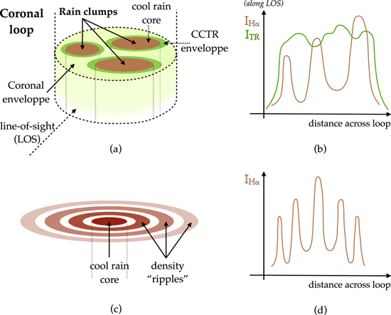
Figure 2. Sketch of the cross-section of coronal rain clumps. Coronal rain clumps are composed of cool and dense chromospheric cores of a few hundred km width, surrounded by a thinner but strongly emitting transition region (that we label CCTR for Condensation-Corona Transition Region) to the coronal enveloppe composing the loop (a). Assuming a LOS transverse to the loop, as depicted in panel (a), a rough estimate of the emerging intensities in a chromospheric line such as Hα and a transition region line are shown on (b). We assume that the small scale structure in the TR line (on the order of a few hundred km) is unobservable with current instrumentation, due to the lower resolution with respect to that achievable in Hα. In the case of rain clumps being thermal modes, perpendicular thermal conduction leads to a transverse density structure in the form of 'ripples' for the thermal mode (c), producing a highly multi-stranded Hα intensity in the transverse direction to the loop (d).
Download figure:
Standard image High-resolution imageWhen observed with a high resolution spectrometer such as the SST, at the smallest observable scales of a 100 km or so, the rain appears multi-stranded in the direction perpendicular to the flow [21]. This structure is observed when following a clump in its trajectory downwards. At every single time during its trajectory the clump appears to have an extended and rippled transverse spatial structure spanning a few Mm overall with individual ripples of a few hundred km widths and with a wider bright core (figure 2, panels (c) and (d)). This structure remains when integrating over a significant wavelength range, and therefore suggests a physical nature related to the mechanism of rain formation (more on this in section 4.2).
2.1.2. Temperature and densities
As noted above, coronal rain is a multi-thermal phenomenon in the sense that it emits in chromospheric and transition region temperature lines (a few 103 K to several 105 K). Besides the main current observatories mentioned in the introduction it is important to note that there is a long history of observations in transition region lines of phenomena associated with catastrophic cooling. Some examples of such work, with Skylab in the Ne VII 465 Å and O VI 1032 Å lines [25], with the Solar and Heliospheric Observatory/Coronal Diagnostic Spectrometer (SOHO/CDS) in the in O V 629 Å line [26] and in the He I 584 Å line [27], in the 1600 Å channel of TRACE [28], in the 304 Å channel of SOHO/Extreme-ultraviolet Imaging Telescope (EIT; [29, 30]), and more recently in the Mg VI 269 Å and Si VII 275 Å lines with Hinode/EIS [31], in the 304 Å channel of SDO/AIA [17] and in the Si IV 1394 and 1403 lines with IRIS (e.g. [32]).
Precise temperature measurements of the cold rain cores have been made through Gaussian fitting of spectral lines [22], particularly precise with simultaneous observations in more than 1 line from elements with different masses [19, 33]. Similarly, an estimation of temperature can be obtained through EUV absorption by neutral hydrogen, neutral and singly ionised helium [21, 34]. These works indicate coronal rain core temperatures of a few 103 K to a few 104 K, with a peak below 104 K. The EUV absorption method also allows to estimate the density of the neutral population. Density measurements can further be made through correlation of absolute intensity of Hα with the emission measure [33, 35]. Through these techniques, coronal rain core total densities have been found in the range of  . The overall emerging picture is that of coronal loops with small cool and dense cores, with thin and elongated boundary shells at transition region temperatures.
The density estimates allow to infer a coronal rain mass flux per loop on the order of 1–5 × 10⁹ g s−1. These values are similar to those obtained for prominences [4] and constitute a significant downward flux of roughly a third of the estimated upward mass flux from spicules. Similar values have been found through seismological analysis of the excitation of (vertically polarised) transverse loop oscillations in coronal loops due to coronal rain [36, 37]. These numbers suggest that material in the form of coronal rain constitutes an important part of the chromosphere-corona mass and energy cycle of the solar atmosphere.
2.1.3. Dynamics
Coronal rain downward total velocities show a very broad distribution, from a few  to a few
  , with a peak at
  [22]. It is important to note that although coronal rain is mostly observed to go downward towards the solar surface along one or both legs of a coronal loop, upward flow on one loop leg followed by downward flow on the other leg (a partial siphon flow with the rain appearing during the event) and also changes of direction (upward/downward along the same leg) have been reported [38].
A peculiar aspect of coronal rain concerning its dynamics is its smaller than free-fall downward acceleration (field-aligned flow). Indeed, several authors with multiple imaging and spectroscopic instruments (able to capture the full velocity vector, not only the plane-of-the-sky component), have reported downward accelerations around or less than 0.1 km s−2 [19, 22, 28, 29, 39, 40]. This is almost a third of the gravitational value, and roughly half the average effective gravity value assuming a circular loop (0.174 km s−2).
Several reasons for these low acceleration values have been suggested, but mainly a ponderomotive force due to transverse MHD waves [39–41] and a gas pressure gradient force [38, 42, 43], with the latter found to be the more effective mechanism. While the heating mechanism of a coronal loop is expected to produce continuous gas pressure variations within a loop, Oliver et al [43, 44] have shown that the very generation of a dense clump in a rarefied medium such as the corona generates a field-aligned travelling gas pressure front enhancing the gas pressure in its wake, rapidly cancelling the downward acceleration. The terminal velocity is found to be solely determined by the density contrast between the clump and the external medium in a remarkably clear relation that has not been analytically explained yet.
2.2. Global properties of loops with rain
To understand the physical mechanism of coronal rain it is essential to understand the global properties of the coronal loop in which it is formed. Coronal rain is mostly reported in active regions, the hottest regions in the solar corona. It should be noted, however, that other types of coronal rain have been reported that involve a loop arcade geometry with null point topology at the top, where either magnetic dips can form and the mass can accumulate and cool [14], or where the loops are long enough and their expansion is large, thereby favouring catastrophic cooling [13]. In the case of coronal rain in more simple loop (active region) geometries, prior to coronal rain appearance, the hosting coronal loop is observed to cool from several million Kelvin temperatures down to transition region and chromospheric temperatures mainly through radiation, a process that takes a time on the order of 1000–5000 s [21]. During this process, accelerated cooling in the transition region temperature range is observed [33, 39]. Progressive cooling of the chromospheric material is sometimes observed, showing more and colder material further down the loop [21], but sometimes also reheating and becoming progressively hotter closer to the footpoint [19].
A major observational finding is that neighbouring field lines of a coronal flux tube tend to show coronal rain synchronously (within a few minutes), across a characteristic transverse length of  [22]. Since these results have been obtained in the lower corona, close to the footpoints, this cross-field time lag may be even shorter at the location of coronal rain formation, close to the apex. Given that a loop is on average observed to have a width of
  , this result is at odds with the general concept of coronal loop evolution. Indeed, a coronal loop is thought to be composed of one-dimensional independently evolving strands (based on the fact that the field-aligned thermal conduction coefficient in the corona is several orders of magnitude larger than the perpendicular component) [45], while this finding suggests that neighbouring magnetic strands within a loop with rain undergo a similar thermodynamic evolution (and quasi-simultaneous catastrophic cooling). A simple explanation to this result is provided by footpoint heating-induced thermal instability, as we will see in section 4.
Observations of flare-driven coronal rain provide further clues to the mechanism behind coronal rain formation. Following the intense electron beam heating in the chromosphere from the magnetic reconnection process, the flaring loop is subject to intense chromospheric evaporation. During the initial stages of the flare the loop cools mostly through thermal conduction, but once chromospheric evaporation occurs and the loop becomes dense, radiation takes over as the main cooling mechanism. In a coordinated observation between the NST and IRIS, Jing et al [23] observe the flare ribbons (locations of electron beam impact in the chromosphere) followed (after a few  ) by the impact of the rain in the chromosphere. As expected, the paths of both the ribbons and the impacting rain coincide. More importantly, the ribbon brightenings, the impacting rain brightenings and the rain widths show the same widths, suggesting that the spatial scale of energy transport in a flare may be reflected by the width of the rain.
Combining the SST/CRISP, SDO/AIA and GOES, Scullion et al [46] observe that once the temperature has cooled below the million Kelvin regime (roughly 30–60 min after the impulsive phase) an accelerating cooling process takes place, in which the cooling rate passes from  to
to  and the rain is then observed in Hα. This accelerated cooling phase is expected since for transition region and upper chromospheric temperatures a significant number of atoms, and in particular hydrogen, calcium and magnesium atoms, start to recombine and become strong radiative sources [47]. These strong cooling sources have important consequences on the thermodynamic stability of the material at short temporal scales (section 4.2).
The observed densities ( ) and mass flux (
 ) for flare-driven rain are found to be one order of magnitude larger than for quiescent rain, clearly reflecting the observed pouring character of cooling flare loops and the expected large chromospheric evaporation that follows the initial electron beam heating. An important open question in flare physics is what exactly produces the coronal rain, and more precisely, whether the electron beam heating alone (leading to chromospheric evaporation and radiative cooling) can lead to catastrophic cooling and rain. Initial results by Reep et al [48] indicate that this is not the case and that a secondary and yet unknown heating source is needed, besides electron beam heating.
3. Long-period intensity pulsations
Using full disk SOHO/EIT data and later on SDO/AIA data, Auchère et al [49] and Froment et al [50], respectively, recently discovered a remarkable phenomenon in the solar atmosphere. Intensity pulsations in basically all of the instruments channels were discovered ubiquitously all over the Sun with varying periods of a few to tens of hours, lasting over several days. Roughly half of these events are located in active regions, where the pulsations concentrate over loop-like geometries.
The detection method is based on the Fourier power spectra, by carefully measuring the background noise spectrum and calculating the 99% confidence level threshold [51]. The regions with pulsations exhibit power on the order of 10s of σ, reflecting the clock-like behaviour of the pulses.
Through DEM analysis, Froment et al [50] show that these pulsations correspond to recurrent cycles of heating and cooling in which the coronal AIA channels capture the cooling trend from several million Kelvin down to temperatures below a million K. Importantly, they find that the temperature precedes the density increase in each pulsation (by the order of  or so), a fact also reflected in the evolution of the DEM slope. As we will see in section 4.1, this is a characteristic signature of the physical mechanism behind the pulsations. Using the timelag analysis technique [52], they further show that the regions exhibiting the pulsations within active regions cool across the million K temperature range covered by the AIA channels in the same way as any other region, showing that the cooling trend in the coronal temperature range is not different (and that therefore their densities should be similar to any other loop). Furthermore, they analyse in detail a pulsating loop and show through numerical simulations that it is likely that the plasma does not go much below
  , and that therefore no coronal rain may form in this loop. This was later checked by Auchère (private communication) using STEREO A & B data of the same loop simultaneously observed off-limb, with very little or none of the characteristic clumpy condensations in 304 that correspond to coronal rain.
A difference in the cooling trend between other pulsating loops and neighbouring non-pulsating regions was placed in evidence by Auchère et al [53] by investigating the entire AIA suite of channels and in particular the regime below the million K, provided by the AIA 304 channel (emitting at  ). The authors show the periodic appearance of coronal rain in the 304 channel during the cooling stage of the pulsations in a transatlantic loop (characterised by being very long). They further show that the emission in the 304 channel increases immediately after a maximum is observed in the 131 channel corresponding to
  , suggesting accelerated cooling.
Although the work does not include chromospheric lines, the observatory at Pic-du-Midi has co-observations of the same event in Hα, which show chromospheric coronal rain (complete condensations) within the same loop (Auchère, private communication). Hence, it is clear that the cooling in this loop is catastrophic, going all the way down to the chromospheric regime.
An interesting finding is that the timelag between the AIA 171 channel ( ) and the 131 channel (
 ) was found to be negligible in the pulsating loop without rain analysed by Froment et al [50] while it was found to be 4–15 min in the pulsating loop with rain in [53]. This small time delay (which could pass ignored) shows that there is accelerated cooling below the
  range, and that one needs to be cautious when using the timelag technique to infer the existence of cooling to transition region temperatures only with the coronal AIA channels (this is particularly true because the AIA 304 channel is often ignored due to its optical thickness).
Recently, Froment et al [33] analysed a unique dataset of a coronal loop bundle with long-period intensity pulsations observed at the limb during a cooling phase with the CRISP and CHROMIS instruments at the SST. For the first time, the intensity pulsations and the chromospheric coronal rain are detected and analysed together, thereby bridging the immense spatio-temporal and thermodynamic scale range. The coronal rain presents very similar morphological, dynamical and thermodynamical characteristics as previous coronal rain events. Even though the pulsations are only detected in a specific loop bundle, coronal rain is observed in a large section of the FOV, in many other loop systems.
As we will see in section 4 the fact that periodic coronal rain is observed together with the long-period intensity pulsations is a major evidence for the physical mechanisms behind both phenomena. The physical interpretation also allows us to understand why coronal rain may be much more prevalent than the long-period intensity pulsations.
4. Physical mechanisms: TNE and thermal instability
4.1. Global evolution: TNE
TNE corresponds to a state of a system that undergoes cycles of heating and cooling around an equilibrium position due to a feedback mechanism. This equilibrium position may or may not be attainable, and the feedback mechanism can involve the boundary conditions of energy and mass input/output, the intrinsic properties such as its ability to cool, or even the heating mechanism itself [54].
In the solar context, as shown by Kuin and Martens [55], such a system can be the combination of a coronal loop and the chromosphere where it is rooted and that acts as mass reservoir. Based on the timescale of thermal conduction, the pressure restoring timescale (sound wave travel time) and the thermal timescale (due to thermal perturbations) the authors show that this system can be seen as one entity reacting simultaneously to variations in temperature (assuming thermal insulation in the chromosphere). The strong coupling between the chromosphere and the corona occurs as follows, and is summarised in figure 3 (for a detailed explanation please refer to Klimchuk and Luna [56]). Thermal conduction is highly efficient at redistributing the excess energy throughout the corona. If a heating event (such as a Parker nanoflare) occurs in the corona, most of its energy is rapidly transported into the thin transition region and chromosphere, where it is radiated away. In the presence of a large downward conductive flux (as in the case of footpoint heating, see further below) the chromosphere can heat up locally, leading to an increase in pressure at the top of the chromosphere and producing an evaporative flux into the corona. If this process is maintained (producing constant chromospheric evaporation) the corona slowly increases in density and starts to radiate more efficiently (due to the density squared dependence). The heating being constant, the energy per unit mass in the corona goes down, bringing the temperature down slowly in time. Since plasmas radiate more efficiently at lower temperatures (in the transition region to coronal range, with a peak at  ) this cooling process can accelerate, a process that is only stopped by the evacuation of plasma into the chromosphere and decrease of density in the corona. The cycle then starts again (provided that the heating source is still active), with a very fast reheating of the loop given its rarefied conditions.
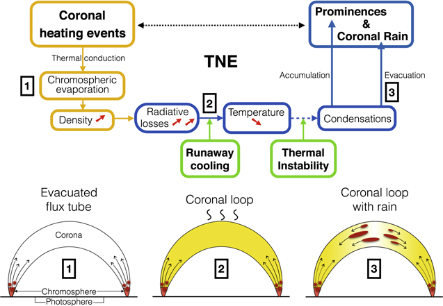
Figure 3. Sketch of a TNE cycle. The cycle contains three main steps, shown by numbers '1', '2', '3'. An evacuated magnetic flux tube is subject to quasi-steady heating events concentrated at the footpoints (red stars in the sketch, number 1 in the figure). Thermal conduction distributes the energy along the flux tube, rapidly heating it up. The energy is mostly transferred down to the transition region and upper chromosphere, where it is radiated away and also heats up the plasma. The local heating leads to an increase of pressure and chromospheric evaporation. Plasma fills the loop, which becomes over-dense and starts radiating strongly. The cooling part of the cycle begins, dominated by radiative losses (number 2). It is a runaway cooling process because of the temperature dependence of the optically thin loss function. Under specific conditions of local thermal equilibrium thermal instability can set in, which leads to the generation of condensations locally in the corona. The condensations can either stay and accumulate to form a prominence, or evacuate downwards under the action of gravity and gas pressure in the form of coronal rain (number 3). The loop is then mostly evacuated and the process repeats if the footpoint heating persists. The main heating and cooling parts of the cycle are illustrated by orange and blue boxes, respectively.
Download figure:
Standard image High-resolution imageUnder specific conditions of heating, the chromosphere-corona loop system can therefore exhibit cyclic variations in temperature-density phase space that can be stable or unstable. A stable solution is one in which the cycles have an attractor to which the cycles converge to in time (a static solution), while an unstable solution is one in which every solution diverges away from the static solution into a nonlinear oscillatory cycle called a 'limit cycle'. Under coronal conditions, Kuin and Martens [55] show that only unstable solutions should exist (exhibiting limit cycles).
Simulations over the last decade have shown that placing a constant, or quasi-constant (i.e. high frequency) source of heating highly localised in the low corona (with a small heating length scale compared to the loop length)—also known as 'footpoint heating'—led to the TNE conditions described by Kuin & Martens (e.g. [57–59]). Indeed, footpoint heating naturally produces a large downward conductive flux that leads to an increase of pressure and chromospheric evaporation (number1 in figure 3), while the apex of the loop is mostly maintained by an enthalpy flux, leading to a corona with increasing density that cannot be in global thermal equilibrium [60]. The loop starts an accelerated cooling process driven by radiation (number 2 in the figure), and under specific conditions discussed below (in which we argue that thermal instability can set in), leads to the generation of condensations locally in the corona. The condensations can then either stay and accumulate to form a prominence [61–63], or evacuate downwards under the action of gravity and gas pressure in the form of coronal rain (number 3 in the figure) [64–69]. The loop is then mostly evacuated and the process repeats if the footpoint heating persists.
It is worth mentioning that condensations can in theory continuously form in the corona due to footpoint heating and fall down leading to a prominence-like, apparent long-term static equilibrium (and prominences do show significant cyclic refilling and evacuation [3, 70, 71]) but it is also thought that magnetic dips play an important role in the formation of large prominences [5]. It is also possible that in the presence of highly symmetric heating and geometric conditions at both footpoints of a loop, the initial large accumulation of dense plasma at the apex of the loop generates magnetic dips that lead to prominence formation [72–74].
TNE cycles produced by footpoint heating are therefore also known as evaporation—condensation cycles, referring to the heating and cooling phases, respectively. Two conditions are thus essential to their existence: a heating function sufficiently concentrated at the footpoints (with a ratio of apex to footpoint heating of 10% or less [56, 60]) and frequent enough (with a timescale faster than the radiative cooling time [75]). Furthermore, Klimchuk and Luna [56] show that asymmetries between both footpoints (of heating and/or area expansion) cannot be too great.
Does a TNE cycle automatically lead to the condensations that characterize coronal rain? Not necessarily, as shown by Mikić et al [76]. If asymmetries between the area expansion at both footpoints are important and/or asymmetries in the heating at both footpoints are important then cool condensations may not form. Indeed, a new kind of solution arises in which strong and recurrent siphon flows sweep away the cooling regions in the corona in a timescale lower than their cooling time. For this reason, such regions are called incomplete condensations and seem to correspond to the loop observed by Froment et al [50]. In the vast parameter space investigation conducted by these authors [77], it is shown that TNE cycles with coronal rain (complete condensations) form in a relatively small part of the parameter space, and that therefore very specific heating and geometric conditions need to be fulfilled to obtain coronal rain. Interestingly, the investigation also shows that for larger heating input at the footpoints, TNE starts to populate increasingly more the parameter space with basically only complete condensations and therefore less sensitivity to the geometric asymmetries. By extrapolating this trend to higher heating input and the flaring regime we can speculate that coronal rain is unavoidable, as indeed flare observations suggest, and that asymmetries play a negligible role in the formation of flare-driven rain. However, for large heating input asymmetries, multi-dimensional effects become important. Indeed, large heating input can generate large shear flow velocities in loop arcades that trigger flow instabilities such as Kelvin–Helmholtz [78]. These instabilities lead to strong heating at the loop tops, thereby inhibiting (or delaying) catastrophic cooling.
On the other hand, simulations indicate that the generation of coronal rain (complete condensations) does seem to require strongly stratified (footpoint) heating over a time interval that is comparable to its cooling time [75]. Based on this, it was proposed that coronal rain could serve as a proxy for coronal heating mechanisms [38]. Indeed, loops without coronal rain would be heated by mechanisms characterised by having highly frequent dissipative events (nanoflares) and being uniformly distributed in the corona (or with large enough heating scale lengths), such as nonlinear Alfvén waves dissipating through shocks [79, 80]. On the other hand, loops with coronal rain would have mechanisms with a footpoint heating nature (a scenario that is more likely with ohmic heating through slow magnetic stress from convective motions, [81, 82]).
The main observational signatures of TNE cycles predicted by numerical simulations can therefore be listed as follows (see also figure 3):
- A fast (re-)heating phase of an evacuated loop to high temperatures (several MK), accompanied by fast upflows.
- A slow cooling phase in which the loop density gradually increases: we have an out-of-phase density increase with respect to the temperature.
- The cooler the EUV channel, the later its intensity will peak during the gradual cooling phase of a loop from a hot coronal temperature. The runaway cooling behaviour translates into shorter timelags between pairs of EUV channels sensitive to cooler temperatures. This scenario is, however, strongly dependent on the LOS superposition and the influence of the Condensation-Corona Transition Region (CCTR) interface.
- The loop evacuates: an increase of downflows is observed at the end of the cooling. These can be either at warm (coronal or transition region) temperatures, case in which the term 'incomplete condensations' is used, or cool (chromospheric temperatures), case in which we refer to 'complete condensations' (or catastrophic cooling) and coronal rain is observed.
We can now see how TNE cycles of heating and cooling, also known as evaporation and condensation cycles, naturally provide an explanation to the observed long-period intensity pulsations. Assuming a quasi-steady source of heating, the clock-like behaviour of limit cycles ensure very high Fourier power. Using 1D hydrodynamic simulations adapted to the observed geometry (recovered through magnetic field extrapolations) in [50], Froment et al [83] show that TNE cycles with specific heating parameters match particularly well the observed thermodynamic evolution of the loop.
A large amount of information on the coronal heating mechanisms may therefore be obtained based on the detailed analysis of observed TNE cycles, and we could thus say that this a new form of coronal seismology, not based on waves but on pulsations. However, the parameter space involved in the shaping of TNE cycles, and in particular deciding their existence, is vast. Both, geometrical factors (loop area expansion, loop length and asymmetries between both footpoints) and the characteristics of the heating mechanism(s) are involved (heating scale length at both footpoints, the occurrence frequency of the events, the presence of an additional background heating), as is clearly shown in [75, 77].
However, as stated in the list above and also in figure 3, TNE not always leads to catastrophic cooling and the formation of coronal rain. Actually, the highly localised character of the rain (its clumpiness) and its very fast occurrence timescale violate the very base of the limit cycle assumptions: the catastrophic cooling is only observed locally and on a timescale faster than the conductive timescale. Therefore the system stops evolving as a whole. It is therefore relevant to ask what determines the formation of coronal rain and whether there is an additional mechanism behind it.
4.2. Local evolution: thermal instability
The plasma in the solar corona is fully ionised and therefore its ability to absorb and reemit energy is strongly limited. At lower temperatures the elements start to recombine and electrons populate increasingly lower energy levels, meaning that its ability to radiate energy is increased. The optically thin loss function, which measures the ability of the plasma to radiate energy, has a roughly exponentially increasing trend with decreasing temperature down to  [84]. Parker [85] and later on Field [86], more rigorously in his seminal paper, realised that this characteristic of plasmas could lead to a catastrophic cooling effect (or thermal runaway) that made plasmas thermally unstable.
In a homogeneous plasma, 4 wave solutions exist: the slow, fast, Alfvén and thermal modes. In his analysis, Field obtained the dispersion relation resulting from a homogeneous and infinite plasma initially in thermal equilibrium and showed that the inclusion of non-adiabatic effects such as net radiative losses over a heating input, influences the slow, fast and thermal modes (while the Alfvén mode remains unaffected). While the slow and fast modes are essentially damped by non-adiabatic effects, the thermal mode can become unstable. The thermal mode corresponds to a non-propagative wave mode characterised by a local temperature decrease and a density enhancement that can occur either in isochoric conditions (constant volume) or isobaric conditions (constant pressure). In astrophysical conditions, and in particular solar corona conditions, it seems that the isochoric instability is more likely [73, 87]. As shown in [88] (see also [89]) the instability can occur for temperatures above ≈5 × 10⁴ K, and the perturbation wavelengths above which the plasma should become unstable are given by the Field's length:
where  and Λ denotes the radiative loss function and, besides temperature, also depends on the ionisation degree ξ for partially ionised plasma. This is because once the material starts to recombine, the energy released (which depends on the ionisation potential) can go into heating the plasma, thereby slowing down the cooling rate [90]. This has an important effect on the temporal and spatial scales of the instability [91].
The analysis of Field was later extended to non-uniform media, with the spatial and temporal characteristics of the thermal instability modes shown to depend strongly on the anisotropy of thermal conduction [92, 93], the alignment of the wave vector and the magnetic field [94], the details of the radiative loss function [95, 96], and the initial conditions.
The catastrophic cooling (exponential growth rates), the accompanying pressure loss in the corona (due to a recombination of electrons) and the resulting local accretion of material to form high density condensations in the solar corona (a medium originally assumed to be roughly in thermal equilibrium) predicted by thermal instability were proposed as explanations for the origin of solar prominences [85] and their lengths based on Field's length [97–99]. The inclusion of perpendicular thermal conduction, even if several orders of magnitude lower than the longitudinal term, was shown to introduce a dense set of thermal modes whose eigenfunctions are spatially multi-stranded (filamentary), perpendicular to the magnetic field, with a local maximum, thereby providing a possible explanation to the observed filamentary structure of prominences [92, 93] and also that of coronal rain [21] (see figure 2, panels (c) and (d)). Analogously to equation (1), a secondary Field's length, or rather, a 'Field's width', could be introduced, linked to the perpendicular conduction coefficient. Since this coefficient is particularly important in partially ionised plasmas, the Field's width would particularly depend on the degree of ionisation of the condensations.
It was however pointed out later by Antiochos et al [59] that the conditions of loops under TNE are never in thermal equilibrium, and, therefore, that the thermal collapse of the corona during a TNE cycle does not correspond to a thermal instability but just a loss of equilibrium, since the conditions for an instability (starting from an equilibrium) are not satisfied. Furthermore, Klimchuk and Luna [56] and Klimchuk [100] argue that the generation of condensations can be explained solely through the physics of TNE (in particular, the exponential cooling rate based on the optically thin loss function).
A proper numerical and analytic investigation that could properly resolve the question of whether thermal instability can take place during a TNE cycle is still missing. However, we here propose an alternative view that resolves this apparent contradiction. Indeed, both views are correct if we consider the timescales and length scales of both processes. While a TNE cycle assumes the loop (chromosphere-corona system) to be a single entity responding simultaneously to perturbations and has usually a period of several hours, the instability can occur over smaller length scales and can have a much faster growth time.
To illustrate this more rigorously we consider a numerical simulation of footpoint heating in a typical coronal loop. The conditions of the numerical experiment are similar to those of Antolin et al [38] ('nanoflare heating function' model in the paper; we refer the reader to this work for further details). In particular, the model consists of an expanding coronal loop of length 100 Mm, with a photosphere and a chromosphere, heated with a stochastic heating function composed of heating events that are randomly distributed in time and space, while being concentrated at the footpoints of the loop (within the length range [2, 20] from the photosphere at both footpoints). The heating events have a maximum duration of 40 s, a heating length scale of 1000 km, a maximum volumetric heating rate of 0.5 erg cm−3 s−1, and occur on average each 50 s. This heating function leads to TNE in the loop accompanied by coronal rain. We show roughly 3 cycles in figure 4. As shown in this figure, the occurrences of coronal rain are characterised by being extremely local in time and space: the catastrophic cooling leading to the chromospheric conditions of the rain occurs in a timescale of minutes, following a much slower cooling rate. The lengths of the rain are on the order of 1000 km, while the length of the corona is at all times close to 105 km.
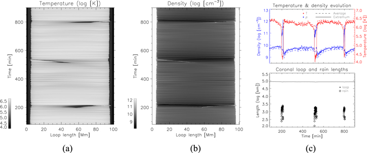
Figure 4. Simulation of a footpoint-heated loop undergoing TNE with coronal rain. The loop is composed of a photosphere, chromosphere and corona, and is heated by a stochastic heating function (see text for details). (a) Temperature evolution, (b) density evolution and (c) time-distance diagrams showing roughly 3 TNE cycles. The average temperature and density in the top panel of the time-distance diagrams are calculated over the coronal part of the loop (length range [7, 93] Mm, regardless of the rain locations), and the extrema denote the minimum temperature and maximum density over this coronal length. The coronal and rain lengths in the bottom panel of the time-distance diagrams are calculated by tracking the transition regions at both footpoints and the sharp density and temperature gradients of the coronal rain. The coronal length excludes the rain lengths.
Download figure:
Standard image High-resolution imageWe argue that towards the end of the cooling part of a TNE cycle, when the temperature in the corona is mostly constant (or dipped at the apex), a coronal parcel of plasma is in pressure balance and in a critical thermal equilibrium locally, with the radiative losses only slightly larger that the enthalpy flux (and the thermal conduction flux in the case of a temperature dip), such that the system is slowly cooling. In such a state, small thermal perturbations cannot be stabilised by conduction, paving the way for a thermal instability [91]. Taking common plasma values found during the cooling part of a TNE cycle, a total number density of  , a temperature of T ≈ 105.8 K with a corresponding loss function value of
  [84], we obtain critical perturbation wavelengths of
  from equation (1), which corresponds to the averaged observed lengths of coronal rain. The growth rates of the thermal mode can be on the order of 10 min or less [89]. Also, the perturbations leading to the instability can come through the interaction with slow modes or fast modes, which are abundant in coronal loops [88]. These order magnitude estimates suggest that the growth time and length scales of the thermal instability match the observed and simulated time and length scales on which coronal rain manifests.
Footpoint heating-driven thermal instability in loops can also naturally explain the observed near-simultaneous occurrence of coronal rain in neighbouring field lines [21]. Since the magnetic field expands in the solar corona, we expect neighbouring field lines to be subject roughly to the same footpoint heating conditions and have similar loop lengths. Hence, once thermal instability is triggered in a given field line, the fast mode perturbations that result can trigger the thermal instability in the neighbouring, critically stable field lines. This process therefore occurs in an Alfvén timescale (on the order of a minute or so) and is shown by Fang et al [101] in 2.5D MHD simulations of a coronal arcade subject to footpoint heating, in a process termed 'sympathetic cooling'. The growth of the condensations is therefore faster in the perpendicular direction than in the longitudinal direction. In this scenario, the width over which coronal rain occurs corresponds therefore to roughly the width of the loop, as is indeed observed, on average ( ). It is also possible that due to their extended transverse scale (the so-called 'density ripples'), the thermal mode itself triggers other thermal modes in the neighbouring field lines.
Hence, in this scenario, thermal instability occurs locally on a system that is globally in TNE. The TNE cycle brings the corona to critical stability but it is the local perturbations (through interaction with sound or fast modes) that drive the growth of the condensation via a thermal instability. If the conditions of the system (heating and geometry) are roughly constant through time and the plasma during the cooling stage is in the appropriate conditions, thermal instability will occur at the end of each cycle, thereby explaining periodic coronal rain accompanying the long-period intensity pulsations. If asymmetries are important in the system, siphon flows can reduce the falling time of the cooling plasma, thereby preventing it becoming thermally unstable and leading to incomplete condensations. In this scenario, the presence or absence of thermal instability dictates the character of the condensations, becoming complete or incomplete, respectively. We can also think of a thermally unstable loop without TNE cycles: consider for instance a loop whose heating conditions are quasi-steady and footpoint concentrated only during a brief period of time (on the order of the radiative cooling time). Then the loop will undergo catastrophic cooling and subsequently collapse if not reheated. The heating and cooling cycle of the loop is then solely dictated by the timescale of the heating in the loop and not by TNE [75]. This scenario may be the most common case for the solar corona, as is observed, for instance by Froment et al [33]. A flare loop also falls into this category, although the exact heating requirements are still unclear [48].
5. Outstanding open questions in the field
With the advent of high resolution and multi-wavelength instrumentation covering the chromosphere-corona temperature range, a new picture of the solar corona is starting to emerge. Besides the generally accepted hot corona, observations are showing a new, cool side of the corona, with ubiquitous coronal rain along with prominences. The occurrence of this phenomena is not due to a lack of heating (flare-driven rain being the prime example of this) but rather because of specific spatio-temporal characteristics of the heating mechanism(s). Therefore, we can talk about a 'cool alter-ego' of the hot solar corona, spanning a new active research community that is not only confined to the solar field. Here are some of the major open questions that are being addressed.
5.1. How much coronal volume at any given time is thermally unstable or belongs to a system in a state of TNE?
While quiescent coronal rain and flare-driven rain are active region phenomena and are observed in every active region, new kinds of coronal rain are being reported, linked to Quiet-Sun regions [13, 15, 102, 103], and are very long-lived [104]. It is now quite clear that coronal rain is a very extended phenomenon. However, a detailed quantification of this phenomenon in the solar corona still awaits. This is important primarily because of the strong link to coronal heating.
How much coronal rain permeates the solar corona and how much of the coronal volume is in a state of TNE are questions that can now be addressed through big-data analysis based on the SDO/AIA and IRIS datasets. It is a far from easy task since it involves the automatic detection of a very dynamic, multi-wavelength and multi-scale phenomenon. Advanced algorithms are however already at hand for this purpose [105, 106].
5.2. How can TNE cycles over several days exist in the solar corona?
The sole existence of a large number of regions in the Sun (both AR and QS) with TNE cycles over days is baffling and poses a major challenge: how can the heating be so steady in time and space, given the far from uniform solar atmosphere subject to multi-scale perturbations? This is further intriguing since magnetic field extrapolations from magnetograms and even large-scale 3D MHD numerical models (that include magneto-convection) show that magnetic connectivity changes happen constantly and that the very concept of a coronal loop seems ill-posed [81, 107, 108]. The very fact that long-period intensity pulsations exist with high Fourier power and with loop-like morphologies is therefore challenging since it suggests the existence of a well-defined coronal loop volume undergoing pulsations. Although 2.5D and 3D MHD models of coronal rain with TNE cycles are now present [68, 69, 82, 109, 110], the loops and coronal rain are not self-consistently formed due to magneto-convection and the heating functions follow specific parametrisation.
5.3. What are the details of the connection between the coronal heating mechanisms and the thermal stability of the plasma?
We know that quasi-steady footpoint heating leads to TNE and thermal instability, that asymmetries in the loop geometries and the heating between both footpoints can produce significant changes in the TNE cycles (leading to no thermal instability), and that more footpoint heating leads to more thermal instability and coronal rain [75, 77]. It is clear that there is a limit to a 1-to-1 relationship between the heating properties and the details of the cooling. For instance, if the heating is too concentrated in the chromosphere and is not large enough, a large part of it will be lost due to the large chromospheric heating capacity and little ability to radiate. Also, the coronal temperature scales with the heating H roughly as H2/7 [111], meaning that the long-period intensity pulsations will only be mildly affected, likely below the instrumental sensitivity. Furthermore, it is possible that other, yet unclear parameters are involved in the TNE and thermal instability occurrence in loops. Particularly, multi-dimensional effects are still largely unexplored. Only recently the first 3D MHD simulations of coronal rain have been achieved [69, 110] (albeit in weak coronal magnetic fields), which show that several dynamic instabilities may be at work (such as Rayleigh–Taylor and Kelvin–Helmholtz). If multi-dimensional effects are not so important for flare-driven rain, we can predict that the more heating at the footpoints, the more chromospheric evaporation there should be and therefore the more coronal rain we should observe. This simple relation should lead to a scaling law between the amount of heating input and the amount of coronal rain within a specific regime of heating conditions (such a relation may have a saturation point at large heating input due to the saturation of chromospheric evaporation [112]). The importance of this relation is clear: extrapolating the scaling law into the largely undetected nanoflare regime (responsible for coronal heating), for which we do observe the quiescent coronal rain would give the bulk, average volumetric heating behind coronal heating. Furthermore, extrapolating (with caution) to the higher energy range would give valuable information about the true flare energy content in stellar flares, for which the signatures of coronal rain may be more readily observed (given also that the gradual phase of the flare is far easier to catch than the impulsive phase).
5.4. What are the observational signatures of the cool side of the corona for the Sun as a Star?
TNE cycles are very dynamic and because they are spatially extended and involve a broad temperature range, from chromospheric to coronal temperatures, it is strongly linked to the intensity variability of the Sun as a Star. Coronal rain-like features such as high redshifts in visible and UV wavelengths have been reported in active stars, particularly the flaring kind [113, 114]. Also, the impact into the lower atmosphere from returning clumps from prominence eruptions and flare-driven rain can produce significant UV emission [23, 115, 116]. It is therefore natural to ask whether quiescent coronal rain from other, far more active stars could be observed as recurrent, highly redshifted signatures in visible and UV spectral lines. We may also ask ourselves about the observational signatures of TNE cycles in these stars. In such cases, the observational signatures would be periodic and may produce false positives in exoplanet detections [117].
5.5. What defines the morphology of coronal rain?
The clumpy and multi-stranded nature of coronal rain is still unclear. The thermal instability mechanism has provided possible explanations for the observed lengths and widths of rain clumps. Shear flows, driven by the loss of pressure in the corona that accompanies thermal instability, also play a large role in their morphology [101]. If the morphology is indeed largely defined by thermal instability then coronal rain constitutes a bridge to understand condensations at much larger scales in the Universe, for which thermal instability is also invoked, such as planetary nebulae [118], molecular clouds in the interstellar medium [119], spiral arms condensing out from the galactic halo [120] and other filamentary structure in the interstellar medium [121, 122]. Similar morphologies and dynamics are also observed in galactic loops [123, 124], structures that may form similarly to solar prominences [125]. Furthermore, the role of condensations formed via thermal instability has been highlighted in star formation processes [126].
It is also possible that at the CCTR interface, significant kinetic effects are in place. Even if the characteristic scales of the plasma (10−5–10−2 m) are much smaller than the typical rain clump sizes, substantial mixing and diffusion processes can occur in this region due to anomalous Bohm diffusion [127]. The faster electron speeds combined with the larger ion Larmor radius can also lead to a charge imbalance across the interface, which in turn generate an electric field across the CCTR toward the condensation. This can lead to the expansion of the condensation into the corona. Different velocity distribution of the chromospheric plasma with respect to the coronal plasma can also lead to two-stream instabilities [128], which can be important for heating.
Since the solar corona is the only space (and terrestrial) laboratory in which coronal rain can be resolved both temporally and spatially, it is in this field that major scientific advancement can be achieved. This is even more the case with the advent of next-generation instrumentation, such as DKIST and Solar Orbiter.
5.6. Is coronal rain a good tracer of the coronal magnetic field topology and its physical processes?
Unlike the previous questions, we do have a reply for this question, and it is definitely a YES. However, the consequences of this are still far from being properly exploited.
As discussed in the previous question, kinetic effects can lead to cross-field diffusion at the CCTR interface. Since these effects are expected only at the interface, we would expect a negligible effect on the overall dynamics of rain clumps. Setting kinetic effects aside, given that coronal rain is partially ionised with a yet unclear ionisation degree, it is fair to ask whether the rain observed in neutral lines such as Hα does follow the magnetic field. The cool emission from coronal rain is likely to originate primarily from scattering of incident radiation from the solar disk, upon which excitation of the neutral atoms is obtained [18]. The coupling between the neutrals and the ions is mainly achieved through collisions in rain conditions, which will depend on the degree of ionisation. For coronal rain we expect a low ionisation degree of 10−5–10−4, leading to a very strong coupling [22]. Even in the case of 50% ionisation, Oliver et al [44] show that a strong coupling would still be obtained, although such case would lead to a significant decrease in the speeds due to the added drag force.
This means that coronal rain can be used as a high resolution tool to elucidate the otherwise invisible coronal magnetic field. Coronal rain can therefore be used to estimate the global magnetic field topology and place constraints on magnetic field extrapolations (or quantify their validity). Spectro-polarimetry of coronal rain can also lead to direct measurements of the coronal magnetic field [129, 130], an aspect that is particularly relevant for DKIST [131, 132]. Furthermore, through observations of coronal rain and prominences we can directly observe coronal heating mechanisms in action. This has largely been demonstrated for transverse MHD waves [39–41, 133] but only recently for heating processes based on magnetic reconnection [134, 135].
The clock-like behaviour of TNE cycles observed over several days can also be used to predict observations of loops under TNE and coronal rain, something particularly useful for scheduling observations of these phenomena.
In summary, the discovery of coronal rain and long-period intensity pulsations has kick-started a fascinating new field in solar physics that is rapidly advancing. We can only speculate that it will become a major driver of solar science within the next few years.
Acknowledgments
PA acknowledges funding from his STFC Ernest Rutherford Fellowship (No. ST/R004285/1) and support from the International Space Science Institute, Bern, Switzerland to the International Teams on 'Implications for coronal heating and magnetic fields from coronal rain observations and modeling' (PI: P Antolin) and 'Observed Multi-Scale Variability of Coronal Loops as a Probe of Coronal Heating' (PIs: C Froment and P Antolin). PA would like to thank C Froment, J Klimchuk, F Auchère, R Oliver, N Claes, R Keppens, the members of the aforementioned ISSI Teams and the anonymous referees for very insightful discussions that greatly contributed to the development of the ideas exposed in this manuscript.
Footnotes
- 1
Note however that very thin and elongated rain clumps (up to
 ) have been observed in Hα [21].
