
Abstract
Plasma jets are sources of repetitive and stable ionization waves, meant for applications where they interact with surfaces of different characteristics. As such, plasma jets provide an ideal testbed for the study of transient reproducible streamer discharge dynamics, particularly in inhomogeneous gaseous mixtures, and of plasma–surface interactions. This topical review addresses the physics of plasma jets and their interactions with surfaces through a pedagogical approach. The state-of-the-art of numerical models and diagnostic techniques to describe helium jets is presented, along with the benchmarking of different experimental measurements in literature and recent efforts for direct comparisons between simulations and measurements. This exposure is focussed on the most fundamental physical quantities determining discharge dynamics, such as the electric field, the mean electron energy and the electron number density, as well as the charging of targets. The physics of plasma jets is described for jet systems of increasing complexity, showing the effect of the different components (tube, electrodes, gas mixing in the plume, target) of the jet system on discharge dynamics. Focussing on coaxial helium kHz plasma jets powered by rectangular pulses of applied voltage, physical phenomena imposed by different targets on the discharge, such as discharge acceleration, surface spreading, the return stroke and the charge relaxation event, are explained and reviewed. Finally, open questions and perspectives for the physics of plasma jets and interactions with surfaces are outlined.
Export citation and abstract BibTeX RIS

Original content from this work may be used under the terms of the Creative Commons Attribution 4.0 licence. Any further distribution of this work must maintain attribution to the author(s) and the title of the work, journal citation and DOI.
1. Introduction
In the last 20 years, many studies have been carried out on atmospheric pressure plasma jets both for the fundamental understanding of the plasma discharge and for their potential applications, as shown in several reviews [1–9] and special issues [10]. Typically, in a plasma jet, a discharge is ignited in a noble gas flowing in a tube (helium and argon being the most used) and the jet expands into air before impacting on a substrate. Many studies have shown that plasma jets can generate high fluxes of reactive species at low gas temperatures. Consequently, their use has been investigated for many different applications, such as polymer etching, food decontamination and treatment of water and biological tissues [6, 8].
In the literature, there is a large diversity of setups for plasma jets with different electrode geometries, various admixtures in the noble gas used, different tube geometries, different flow rates and distances between the plasma generation and the substrate. Furthermore, various excitation sources have been used, with frequencies ranging from Hz to GHz and diverse voltage shapes, including pulse-modulated radio frequencies and dual-frequency excitation. These parameters allow to study and control the discharge propagation and the jet output for applications. One of the most common setups for plasma jets is a coaxial dielectric barrier discharge operated in the kHz regime. However, it is interesting to mention that, a few years ago, different groups defined a common setup working with RF excitation, named the COST reference microplasma jet [11]. Another well defined setup is the kINPen [12]. Using 1 MHz, the kINPen's operation frequency lies between the kHz regime typically used for dielectric barrier plasma jets and radio frequencies.
In this topical review, we focus on kHz helium plasma jets and their interaction with surfaces. This choice of gas and excitation source has been widely studied and guarantees both reproducible and stable discharge generation and negligible gas heating that is essential for biomedical applications [13, 14]. Typically, in all kHz plasma jets, the plasma exits the tube where it is generated as a visible plume of up to a few centimetres long. Even if the plasma jet luminosity seen by the naked eye is continuous, it has first been shown by Teschke et al (2005) [15], Lu and Laroussi (2006) [16] and Sands et al (2008) [17] that it is originated by ionization waves travelling at high speeds of the order of 10–100 km s−1, crossing a few cm in hundreds of ns or in μs timescales. It is interesting to notice that time-resolved imaging of the kINPen jet reveals that even at 1 MHz operating frequency, the discharge also propagates as an ionization wave. As such, many features of discharge dynamics are common to different jet sources and frequencies. It is interesting to note that many early studies on kHz plasma jets have been done using AC applied voltages.However, as the amount of surface charges deposited on the inner surface of the dielectric tube may vary in space and time, it is very difficult to accurately know initial conditions of transient discharges when a sinusoidal voltage is used. use of pulsed kHz sources of positive or negative polarities in experiments has therefore been very helpful to develop comparisons of measurements with simulations. In early experimental [15–17] and numerical [18–22] works on plasma jets, it has been found that the ionization waves in jets are very similar to streamers, although guided by the buffer gas channel, and are typically referred to as guided streamers. These ionization waves are transient but much more reproducible than classical streamers in air, without the complexity of streamer branching. Therefore, the study of plasma jets is also from the fundamental point of view a very unique opportunity to better understand streamer physics from its ignition to its interaction with surfaces.
Early experimental studies were based on the measurements of the discharge current and emitted light intensity. Therefore, first comparisons between experiments and simulations were limited to macroscopic quantities such as the velocity of the ionization front. More recently, more sophisticated diagnostics have been used and allow to measure the electric field and electron density, providing the opportunity to carry out spatially and temporally resolved quantitative comparisons between simulations and experiments. These quantities allow a better understanding of the discharge dynamics and are also the key quantities that drive the production of active species of interest for plasma jet applications.
In this topical review, we focus on recent advances based on the complementarity between experiments and simulations on the knowledge of the distribution in space and in time of electric field, mean electron energy and electron density in plasma jets. We address the influence of different parameters on discharge dynamics, particularly of surfaces, both tube and targets, with different electrical character. The paper is organized as follows: in section 2, we present specificities of diagnostics and models used to determine the reduced electric field, the mean electron energy and the electron density in plasma jets. Then, section 3 is devoted to the general understanding of discharge dynamics in plasma jets. Its subsections address the details of the different temporal stages of discharge evolution, from ignition to interaction with different targets. In section 3, we use mostly simulations to show through a pedagogical approach, with a setup of increasing complexity, the role of the tube, the electrode geometry, the gas mixing and the target on discharge properties. Section 4 focuses on the quantification of the main discharge parameters through the different phases of discharge evolution and on comparisons between simulations and experiments. Comparing experimental and modelling results is necessary for validation, however examining the differences also often leads to understanding what exactly is being measured or modelled by different techniques, making comparisons an essential component of scientific advancement. Section 4 is mostly focussed on coaxial helium kHz jets with rectangular pulses of applied voltage, with rise-time of 10s of ns and width of 100s of ns or a few μs. We end with an outlook and an overview of open questions on the physics of plasma jets interacting with surfaces in section 5.
2. Diagnostics and models to study the dynamics of plasma jets
2.1. Diagnostics for electric fields and electron properties in helium plasma jets
This review is limited to the fundamental properties of non-thermal plasma jets that govern their behaviour and structure in time and space. The experimental diagnostics discussed in this section are therefore limited to electric field and electron properties, because they are affected by the properties of plasma jet source design (gas flow characteristics, capillary tube geometry, tube-target distance, target geometry and electrical characteristics), but are also the fundamental building blocks of the physics of plasma jets. Techniques such as laser induced fluorescence, cavity ring down Spectroscopy, mass spectrometry or infrared and UV absorption spectroscopy which can be used in plasma jets but aim to measure chemical species produced by the plasma will not be discussed here as the production of chemical species is primarily controlled by electron properties. These techniques can however be found in other review papers such as the ones gathered in the special issue 'best practices for atmospheric pressure plasma diagnostics' [23].
In the following subsections, some attention is given to comparisons of data from different sources. The comparison of experimental and modelling results will be discussed in sections 4 and 5.4. When comparing data, either between experiments or between experimental and modelling results, it is essential to take into account the spatial and temporal resolution of the different data sources and to compare it to the spatiotemporal evolution of the studied plasma characteristic.
2.1.1. Electric field
Electric field diagnostics for non-thermal plasma jets can roughly be divided into methods using active spectroscopy, optical emission spectroscopy (OES), methods based on electro-optic effects and a combination of emission spectroscopy and various versions of collisional radiative models.
A frequent example of the latter is combining OES on the spectrum of nitrogen (although using other systems is also often done) and calculating the electric field in the system from the line intensity ratios of selected lines [24]. The ratio depends on the population density of the upper states of the associated lines, which can be computed in a collisional radiative model. Emission lines from different systems can also be used when working in gas mixtures. Finally, the lines used in this method are typically those originating from levels that are populated by direct electron impact. As the associated reaction rates thus depend on the electron temperature, which is a function of the reduced electric field, this method is also suitable for the determination of electron temperature [25]. The positive side of this approach is that information can be obtained using setups that are cheaper, simpler and easier to set up and to use than those of other methods. Moreover, pre-calculated relationships between intensity ratios and the reduced electric field can be used [26]. In addition, vast improvements in the quality of the results are attainable by improving the detection arm of the setup; a good example of extreme temporal accuracy in an erratic system is the use of cross-correlation spectroscopy in the detection arm of the setup, resulting in data that is otherwise challenging to obtain [27]. Still, the associated collisional radiative models of nitrogen or mixtures with nitrogen are complex and the sensitivity of the results to the conditions under which the discharge is measured and modelled should be central when comparing results [28–30].
An emission spectroscopy technique specific to jets in helium is the OES on the Stark-shifted forbidden He lines. In general OES probes the region of the discharge emitting light, which in case of kHz-driven jets is the head of the discharge, very closely linked to the ionization wave. Generally speaking, transitions exist that are forbidden by selection rules under unperturbed conditions. When a strong electric field is present these lines start appearing and shifting in the spectrum as a function of the electric field strength. A method based on the theory by Foster [31] has been later developed by, among others, Kuraica and his team [32–35]. It has been used extensively on He jets that are freely expanding or interacting with substrates [36–49]. That research has revealed that the gas flow speed, being approximately five orders of magnitude slower than the speed of the ionization wave constituting the kHz discharge, still has a fundamental role in the determination of the properties of the discharge. It has been shown that the electric field grows with the distance from the capillary, but also that this phenomenon depends critically on the gas mixing in the effluent of the jet, which is determined by the gas flow speed [43]. In the interaction with substrates it has been shown that the presence of the substrate causes an increase of the electric field just above the surface of the target [46, 47], through two effects: the redistribution of the equipotential lines at the interface and the narrowing of the He channel near the surface. However, if the gas flow is high enough to form a wide footprint on the interface, then the presence of the target does not increase the local electric field with respect to the freely expanding jet [46]. More details about the role of gas flow and targets on electric field profile observed experimentally will be given in light of modelling results in sections 3.3 and 3.4.
Active spectroscopy techniques most used on jets are CARS (coherent anti-Stokes Raman spectroscopy) based four-wave mixing [50, 51] and electric field induced second harmonic generation (E-FISH) [52, 53]. Of the two, E-FISH is simpler to implement. However, both methods have shown impressive results in electric field measurements, especially considering temporal and spatial resolution of the measurements [54, 55]. While in OES-based techniques the resolution is determined by the detection-arm of the setup, in this case the properties of the used laser pulses allow for significant improvements and sub-ns temporal resolution. In addition, active techniques offer the opportunity to measure across the entire structure of the discharge, not only the light-emitting part. However, both methods depend on the susceptibility of the gas under investigation. Consequently, both are predominantly used on nitrogen discharges and are difficult to use on helium. In addition, the influence of the laser beam on the discharge is not always negligible and should be a point of attention [56].
While the electric field in the gas phase is determined by the free charges in volume that make up the discharge and the Laplacian potential distribution, the introduction of surfaces exposed to a plasma leads to the consideration of the effect of surface charges on the electric field. As such, most used techniques for the measurement of the electric field inside dielectric targets are based on the Pockels effect. A relatively simple technique is based on the Sénarmont setup and is capable of measuring only one component of the electric field vector. It was developed for the interaction between streamers and dielectric surfaces [57–65] but has since also been applied to plasma jets [66–69]. This version of the setup is relatively easy to implement and, assuming an ideal configuration, the calculation of the electric field component in question is straightforward and independent of the type of gas. However, imperfections in the setup cause errors in the calculated electric field when the polarization state of the probing light beam is not fully characterized. A more complicated method involves the use of Mueller polarimetry in combination with the Pockels effect, where a complete set of information on the polarization state of the probing light is obtained, revealing all the components where the electric field information is stored [70–74]. In addition, this method allows for the use of imperfect, depolarizing targets, making it possible to measure the electric field in targets closer to application [74]. Furthermore, commercial probes that measure the electric field on the basis of the Pockels effect are available for use on non-thermal plasmas. In this case the Pockels element is not in direct contact with the plasma and the electric field has to be inferred from the relative position of the probe with respect to the plasma [75–77].
Except for the case when commercial probes are used at a distance from the plasma jet to measure only the surrounding electric field, when the plasma is in direct contact with the electro-optical crystal (whether for Pockels or Mueller polarimetry methods) the electric field detected is the one induced by charge interacting with and deposited on the dielectric. The results are, therefore, somewhat different than those obtained by techniques described previously. Indeed, the techniques based on OES or active gas-phase spectroscopy will result in the electric field profile almost exactly reflecting the dynamics of the integral emitted light from the discharge, meaning that the high electric field front will follow the same trajectory as a function of time as the emitted light, within the limits of the resolution of the measurement setup. In contrast, Pockels-based techniques show the electric field footprint inside the dielectric. The charge and the electric field footprint appear with the same dynamics as the light emitted from the surface discharge, but unlike the emitted light, they typically remain until polarity change from the voltage source takes place.
In addition, it should be noted that the discharge growing in the gas phase has a different electric field profile than that interacting with a target. Modelling results show a fast redistribution of charge and equipotential lines as soon as the discharge reaches a dielectric target. Therefore, the comparison of gas-phase data and the data measured on the surface, even if the gas phase data is measured just above the surface, is not straightforward. Pockels-based diagnostics for the determination of electric field inside a target and surface charge require specific electro-optical materials like the BSO (Bi12SiO20) crystal. This material has a dielectric constant of 56. Simulations have shown that when the dielectric constant of the target is greater than four the experienced electric field inside the target is governed by surface charges, while if it is lower the free volume charges play a role as well [78].
In an attempt to give an overview of the experimentally determined electric field data, results obtained with different techniques in the plasma (but not inside the target with electro-optic crystals) have been gathered in figure 1. On the left-hand side the data of the freely expanding jet is gathered [24, 35, 39, 43, 44, 47, 52, 79, 80], while in the graph on the right-hand side the jets are impinging on targets [36, 38, 47, 49, 53]. The x-axis of the left graph is scaled with the gas flow speed. The reason for this is that within a few cm from the end of the capillary, for the flow speeds typically used in plasma jets, this scaling is likely to reflect the gas composition for a given gas type. To demonstrate this, the graph in the inset on the left shows the gas composition by means of air fraction as a function of the distance from the nozzle scaled to the gas flow speed. The data has been taken from the work by Sobota et al (2016) [43], from the results of a simulation of gas mixing of He freely expanding in air. The simulation has been done for particular jet dimensions and flow speeds, thus the validity of the approach can only be inferred to the electric field results from works using the same jet. However, the results do show that close to the end of the capillary, the distance from the nozzle scaled with the gas flow speed does reflect the gas composition.

Figure 1. Experimental values of electric field strength as function of the distance from the nozzle divided by the gas flow speed calculated at the exit of the nozzle considering the gas flow and the tube inner diameter. The left panel (a) shows data for the freely expanding jet, and the right panel (b) shows data for jets impinging on a target. On both figures (a) and (b) the symbol shape corresponds to different powering voltage types with sinusoidal  , rectangular pulses ■, ns-pulses ⋆. The symbols edge colours from blue to red on figure (a) correspond to the range of gas flow velocity from 0 to 8 m s−1 with the same jet taken from [35, 43, 47]. The face colour of other symbols corresponds to
  [39],
[39],  [78, 79],
  [44],
[44],  [24],
[24],  [52]. On figure (b) the colours are related to the type of targets:
  for
for  ,
,  for
for 
 ,
,  for
for  ,
,  for
for  meaning saline water. Solid symbols
  are for grounded targets and open symbols ○ designate floating potential targets. The
  squares with
  edges are ITO coated glass placed on top of grounded metallic plate.
Download figure:
Standard image High-resolution imageAs shown in a number of papers, the electric field strength grows with the distance from the nozzle. The left graph in figure 1 shows that the electric field strength is likely a function of gas composition, as almost all data gathers along a unique line, for both square pulse voltages and sinusoidal ones. This confirms the strong influence of air entrainment on the electric field value. For large gas velocities, the electric field value tends to be slightly higher, which can be explained by the fact that these data correspond to gas flow values at which turbulence starts appearing, leading to higher air admixture at a given position. The opposite trend is observed with the kHz argon jet for which the electric field has been measured by E-FISH [52], shown in green inverted triangles in figure 1(a). This can be caused by several effects, such as the Ar jet consisting of branching streamers, while the kHz He jets feature guided streamers. The random nature of streamers makes it difficult to collect all data from the same position in the ionization front. E-FISH as an active technique is able to collect data from all points in space, unlike the OES-based technique used for the most of the other data in this figure. The red square data in the top left corner of the figure are from [39]. An important addition to the setup in that work was a grounded (or biased) cylinder around the effluent of the jet, which influences the electric field profile, as was also shown in that article. The data denoted with violet circles and triangles are from [24]. Both have been obtained in the same jet. The triangles were measured with an electrical probe on which the jet is impacting at variable distances from the nozzle. The circles were obtained from N2 and  line ratios. The values in this case have been divided by 5 in order to be able to appear on this figure. There could be several reasons for this discrepancy, for example the complexity behind the population mechanism of excited N2 and
  levels, especially in interaction with He [29, 30].
The graph on the right-hand side shows the electric field data when a target is present. Overall, the electric field strength shows the same behaviour as in the freely expanding jet, with the exception in the areas just next to the targets, where a sharp increase of the electric field strength is observed. This is caused by the redistribution of the electric field lines at the interface and the narrowing of the He channel at the interface, as will be detailed in section 3.4. Again the majority of data falls on the same line, showing clearly the dependence of the electric field strength on gas mixing. The data obtained by the E-FISH method [53], shown here in blue triangles, was obtained in an atypical jet system comprised of two surface dielectric barrier discharges joined together to form a large rectangular nozzle. This peculiar configuration allows to increase the interaction length between the helium plasma and the laser beam to increase the weak E-FISH signal induced by helium susceptibility. The discharge is ignited in a helium flow above liquid target. As the gas flow configuration is completely different than for other jets in this graph, the gas velocity has been multiplied by 20 in order to be able to visualize the data.
2.1.2. Electron properties
Electron properties, such as electron density and temperature or energy distribution can be measured or inferred by more methods than the electric field. For example, electron density can be estimated from current measurements [81], but it can also be measured by microwave interferometry [82] or microwave cavity resonance spectroscopy [83] or electrical probes, taking care that they do not alter the discharge. Still, just as is the case for the electric field, directly measuring electron properties in jets is not simple due to their highly transient nature, small size, significant jitter and to low electron densities. That is why trusted methods are borrowed from diagnostics on plasmas that are significantly different from plasma jets, like low-pressure steady-state plasmas.
One OES technique for the measurement of electron density is Stark broadening [82, 84, 85]. It can be applied to atomic lines of different gases like oxygen, nitrogen or hydrogen. The idea is that just like in any general type of collisional line broadening, the interaction between the system under observation (our probed atoms) and the perturber results in a shift in the atomic energy levels. In the case of the interaction of a radiating system and a charged particle, the interaction is of the Coulomb type and the resulting broadening of emitted spectral lines is a function of the density and the temperature of the perturber. The method, thus, relies on the electrostatic interaction between particles, but it also assumes that this field originates only from the charge in the close vicinity of the emitting atoms, a 'microfield' [86] in an otherwise neutral medium. This is crucial, as plasma jets in the kHz region comprise of propagating ionization waves with high electric fields in the head of the discharge, complicating the analysis. Low electron densities complicate the analysis further, as has been discussed in several works [84, 87].
Thomson scattering is an active technique for the determination of electron properties in plasma jets [48, 88–99]. Scattering light on a plasma results in Thomson scattering, Raman scattering (in case of a molecular gas) and Rayleigh scattering, the latter largely dominating the signal intensity. Methods exist to filter out the component belonging to Rayleigh scattering. This is necessary since it is a multitude of orders bigger in magnitude and therefore completely overshadows the other two components. Thomson-scattered signal belongs to the free electrons in the system, if we limit ourselves to non-thermal plasma jets, but appears in the same spectral range as the Raman-scattered signal. If the signal from Thomson scattering is intense enough, a fitting procedure can separate its contribution from the signal from Raman scattering. The intensity of the signal depends on the particle density and its shape on the electron energy distribution function (EEDF). In atomic plasmas it is therefore also possible to determine the EEDF, while in molecular plasmas a Maxwellian distribution is typically assumed. As the intensity has to be high enough, the minimum detectable electron density is around 1019 m−3, but the actual limit depends on the Thomson scattering setup. The method is difficult and expensive to set up, however, electron properties can be measured directly, regardless of the presence of high electric field in the front or other discharge parameters. There are several operational difficulties. For example, the cross section for Thomson scattering is very small, meaning that the integration times in measurements can be very long. One solution is an increase of the intensity of the scattered light, however, this can disturb the discharge. Another issue is that the jitter associated with all non-thermal atmospheric pressure plasmas in combination with a very thin ionization front with high density gradients in plasma jets results in measurements that probe the electrons over the entire volume of the ionization front and somewhat after it. The resulting measured electron properties are thus still not resolved over the head of the discharge and often the electron densities are examined in the channel behind the front. This has big consequences on the electron temperature, that is more likely to reflect the lower-energy electrons just after the head of the discharge instead of the high-energy electrons at its tip [96].
Figure 2 shows an overview of the electron density data from the literature. Data is taken for jets with different excitation sources and buffer gases, since there is few data available for kHz He jets and it is useful to compare it with other jet sources. The data spans over six orders of magnitude. There is quite some data available that is not axially resolved along the plume; in those cases in figure 2 the data is represented by values at x = 0, with minima and maxima connected by a straight line. Furthermore, the articles showing the radial profile of electron density are here represented by the maximum value only. Other papers provide the time evolution of electron density at a given position along the plasma jet. In this case, data are represented with a shaded vertical column at the corresponding position, with the minima and maxima points connected by a straight line. A variety of methods is used for the determination of the electron density and most of them are not direct measurements. Nevertheless, the densities belonging to Ar jets are on average higher than those in He jets, which had been stated by Hofmann et al (2011) [100]. Furthermore, the measurements in He show that the electron density profile follows the electric field profile, discussed in the previous subsection. Both the calculations of electron density from the electric field profile in Sretenović et al (2017) [44] and Thomson scattering measurements [91, 94, 96] give a rising trend of the electron density as the distance from the exit of the capillary increases. The only exception is the decaying trend of electron density measured in [101] with the broadband emission of neutral bremsstrahlung, which could be influenced by the volume of plasma actually emitting this radiation.

Figure 2. Experimental values from literature of electron density as function of distance from the nozzle located at x = 0. Power sources: kHz sinusoidal  rectangular pulses ■, short ns-pulses ▴, + RF. The symbol colours are related to the type of targets:
  for
for 
 ,
,  for
for  ,
,  for
for  ,
,  for
for  meaning saline water. Open symbols
  are for grounded targets and solid symbols
  designate floating potential targets. The shaded blue area corresponds to jet running in helium while shaded yellow area are in argon. Coloured boxes around first author's names designate the measurement method used. Straight lines connect minima and maxima values in series of data. Data are taken from [44, 48, 89–91, 94–101, 104, 105, 107–115].
Download figure:
Standard image High-resolution imageFigure 2 shows a wide range of electron densities measured in He operated jets. To analyse the differences between the results, the maximum value of the electron density of a spatial or temporal series is compared between the various works. The lowest ne,max values are reported by Karakas et al (2012) [102] and Kieft et al (2004) [103] with respectively 3 × 1010 cm−3 and 7 × 1010 cm−3. These values have been estimated using the detected current signal and by estimating the average cross section and average drift velocity. Where Kieft et al (2004) [103] examined a radio frequency-powered plasma needle without an extended plasma plume commonly seen in a plasma jet, Karakas et al (2012) [102] did investigate the plume of a He jet powered by 2 μs high voltage pulses of 5 kHz. The value of 3 × 1010 cm−3 is based on a current peak of 10 mA, a cross-section of 0.39 cm2 and a drift velocity of 5.6 × 10⁴ m s−1. Slightly higher values of electron density are shown in Sretenović et al (2017) [44] up to 1 × 1011 cm−3, estimated through measured electric field values based on Stark shift of forbidden helium lines. This jet has an inner AC powered electrode with an outer grounded ring, rather than two external rings as in Karakas et al (2012) [102], as well as a slightly thinner inner tube diameter (2.5 mm compared to 3.0 mm) which affects the electron density, as will be shown in section 3.2.1.
Values of 5 × 1011 cm−3 have been measured through Rayleigh microwave scattering by Lin and Keidar (2016) [104] for a freely expanding He jet with inner electrode. Additionally, it can be seen from photographs that their plume is much longer than shown by Sretenović et al (2017) [44]. This can be a result of the higher He flow used (5 slm compared to 1.5 slm) and/or lower operating frequency (16 kHz compared to 30 kHz), which can influence the amount of leftover charges present for the next HV cycle. A different AC operated plasma jet has been examined by Yambe et al (2015) [105], which estimates ne,max = 1–5 × 1012 cm−3, based on a measured current of 10 mA, a drift velocity of approximately 10 km s−1 and a cross-section of 0.01 cm2. The large difference with e.g. [102] comes from the estimation of the cross-section, which is much smaller in [105], since the investigated ionization wave travels in a thin ring rather than a 'bullet'-package through the plume.
Higher values have been detected using Thomson scattering by Hofmans et al (2020) [96] and Hübner et al (2014) [91], of 1 × 10¹³ and 2 × 1013 cm−3, respectively. These works have investigated pulsed helium jets instead of AC powered ones and the rise in electron density can also be noticed through an increase in detected current (180 mA [106]) and through a drift velocity of 8 × 10⁴ m s−1 [48]. The same jet as in Hofmans et al (2020) [96] has been examined by Klarenaar et al (2018) [94] when impacting various surfaces like glass and metal. An increase of electron density towards 3 × 1013 cm−3 has been shown when interacting with glass (close to the surface) and towards 1 × 1014 cm−3 for a metal target at floating potential.
Recently, another laser based technique has been used by Lietz et al (2020) [107], called laser-collision-induced fluorescence (LCIF). A laser at 389 nm is used to excite He to the He(23 S) metastable state which is then excited in the plasma by electron impact to He(33 P), whose radiative relaxation is monitored to deduce the electron density. The data from [107] shown on figure 2 have been obtained with a pure He flow and a shroud gas of He containing 5% H2O expanding in a vacuum chamber pumped down to 600 Torr. Despite this peculiar configuration, the measurement shows an increasing profile of electron density with distance from the nozzle similarly to all Thomson scattering data obtained in He jet at atmospheric pressure.
Using Stark broadening, a ne,max = 5 × 1013 cm−3 has been observed by Hofmann et al (2011) [100] for a He RF powered jet with a grounded metal plate (with a hole at the axis of the plasma jet) in front of the jet. This particular electrode configuration is very unique and therefore difficult to compare with other plasma jet systems.
Two different He pulsed systems have been examined through Thomson scattering by Jiang et al (2019) [95] and Wu et al (2021) [98], both revealing high electron densities of 1 × 10¹⁴ and 1–4 × 1014 cm−3, respectively. Although these high values are remarkable for helium plasma jets, they are plausible when considering the power delivery to the plasma. Jiang et al (2019) [95] have operated their freely-expanding jet with a low 10 Hz frequency and pulses of less than 200 ns delivering up to 2 mJ per pulse, which is much higher than for instance the 10–40 μJ per pulse reported in [106] for the jet used in Hofmans et al (2020) [96]. Wu et al (2021) [98] have operated their jet at a comparable 8 kHz but their reported current of 500 mA is much higher than in the other works.
Lastly, high electron densities have been observed inside the capillary tube in two He AC powered jets: 9 × 1013 cm−3 in Tschang et al (2020) [116] and 1–8 × 1014 cm−3 in Jõgi et al (2014) [110] inside the capillary tube. The first case is unique since it is the only jet examined (through N2 line ratios) in the presence of a strong external magnetic field (2 Tesla) impacting on a small liquid target [116]. Jõgi et al (2014) [110] have reported the highest values but comparison with the other papers is difficult since the densities are examined inside the capillary tube of a micro-plasma jet with a small inner diameter of 80 μm. Section 3.2.1 will show that this has a significant effect on the electron densities.
For Ar operated jets, figure 2 shows a wide range of electron densities as well. Similarly as for the helium results, these densities are not only the maximum obtained in a measurement series but also the spatially and temporally resolved results. To compare the various results, the maximum reported electron density of each paper will now be discussed. The lowest ne,max for an Ar jet has been reported by Hübner et al (2013) [90] with 7 × 1013 cm−3. The streamer investigated in that work has been generated by an applied pulsed voltage (5 kHz, 500 ns) to a 1 mm needle housed in a glass tube with 1.8 mm inner diameter and 3 mm outer diameter. The distance from the tip of the needle to the end of the glass tube is not mentioned in the text, but from a photograph an estimation of 3 mm can be made. As a result of this short distance, there is little charging of the glass tube before the ionization wave propagates away in the argon–air mixing plume region.
Slightly higher ne,max values of 1 × 1014 cm−3 have been reported in [100, 109, 111]. These works include plasma jets of various designs but all are operated using voltages with a high frequency, i.e. radio-frequency or microwave. Another radio-frequency operated argon plasma jet has been reported by van Gessel et al (2013) [89] with values of electron density ranging between 1–3 × 1014 cm−3. This RF-jet is modulated at 20 kHz with a duty cycle of 20%, thus with a repetitive plasma on- and off-times of 10 and 40 μs. The aforementioned Ar papers all examined a free-expanding jet without the presence of a target.
Qian et al (2010) [108] have reported maximum electron density values of 2 × 1014 cm−3, for a 38 kHz AC powered jet interacting with a glass target which is electrically grounded on the backside. A different AC powered jet (23 kHz) has been examined by Slikboer and Walsh (2021) [97] interacting with a liquid target (tap water), which yields maximum electron densities in the centre of the plume of 6 × 1014 cm−3 when the liquid is at floating potential and 1 × 1015 cm−3 when grounded. The same jet has been examined for a pulsed applied voltage (16 kHz, 5 μs on-time) in [99], measuring ne,max values of 1 × 1015 cm−3 with a floating potential liquid and 3 × 1015 cm−3 when electrically grounded.
It is worth mentioning that Thomson scattering measurement performed in atmospheric pressure glow discharge in He [93] or in Ar [88] report respectively electron density of 2.5 × 1015 cm−3 and 8 × 1014 cm−3, corresponding to a similar range of electron densities as observed in RF or kHz plasma jets despite a very different type of discharge. In [82], electron densities of 5 × 1014 cm−3 are measured in an Ar microwave surfatron jet source with both microwave interferometry and Hβ line broadening showing a good agreement between values obtained by these two techniques.
Whereas all the aforementioned papers have either used Stark broadening or Thomson scattering to determine the electron densities, the measured current has been used by Sup Lim et al (2020) [113] to estimate an electron density of 2–10 × 1015 cm−3 for an AC operated jet (50 kHz) impacting a small liquid reservoir in a cuvette. Besides the different diagnostic technique used, this jet is different from the others since it has a long quartz tube with a significant gap of 60 mm between the powered inner electrode and the edge of the tube.
Even though a wide range of electron densities has been reported for Ar plasma jets of different design and operating parameters, patterns can be found. Freely expanding RF-jets generate lower electron densities than AC or pulsed jets interacting with a surface. Results from Slikboer and Walsh (2021) [97, 99] using the same plasma jet and liquid target suggest that using a grounded target yields higher densities than a target at floating potential. They also suggest that AC powered jets have lower electron density than pulsed jets, similarly to what is observed for helium plasma jets. However, the works reported by Hübner et al (2013) [90] and by Sup Lim et al (2020) [113] seem to contradict this, which could be related to the significantly shorter and longer distances between the inner powered electrode and the edge of the capillary tube, respectively. The influence of this distance has not been investigated further experimentally. In fact, the only results reported inside the capillary tube (in between the electrodes) instead of the plasma plume are those of Schäfer et al (2010) [112], reporting values of 2–4 × 1014 cm−3 for an RF-operated Ar jet.
2.2. The specificities of modelling helium pulsed plasma jets
After optical imaging of plasma jets revealed ionization waves travelling at high speeds of the order of 10–100 km s−1, the first models of plasma jets have been based on fluid models to simulate streamer discharges [18–22]. The concept of streamer discharges has been put forward by Meek, Raether and Loeb [117–121], as filamentary plasmas that propagate in a uniform gas driven by their own space-charge electric field. In the following sections, we focus on specificities of modelling plasma jets, starting with the setup geometries in section 2.2.1. Then, in section 2.2.2 we focus on the neutral gas flow modelling and helium–air gas mixing. In the last decade, many groups have developed fluid models for plasma jets, such as those in [18, 19, 21, 22, 122–131]. Due to the cylindrical symmetry of the studied systems, most simulations of single plasma jets are done using two-dimensional cylindrical axisymmetric fluid models. Simulations of jets in curved tubes and in tube arrays are performed in 2D Cartesian coordinates [132–135]. Simulations focussing on the chemical kinetics in plasma jets can employ zero-dimensional and 1D models [136–139]. In this review, we focus on the discharge dynamics in single plasma jets. There are two types of fluid models typically used for the discharge in plasma jets: the simplest one based on the local field approximation (LFA) and a more accurate one, based on the local mean energy approximation (LMEA). These will be described in section 2.2.3. Then, in sections 2.2.4–2.2.6 we provide more detailed descriptions of plasma chemistry in helium-based jets, initial conditions, photoionization and the modelling of plasma–surface interactions.
2.2.1. Setups and boundaries
There is a large variety of atmospheric pressure plasma jet designs as seen in section 2.1, including electrode configurations that have pin and ring electrodes either outside or inside of the dielectric tube forming the jet, or some combination of electrodes located inside and outside [6]. Glass tubes are usually used, with variable length and diameter. In each design variation, an ionization wave propagates through and out of the tube and into the ambient air. A rare gas is usually flowed through the tube, either pure or with a small (<1%–5%) admixture of a molecular gas such as oxygen, nitrogen or water vapour.
There is also a large variety of targets used in experiments. In this work, we focus on solid targets. In models, the description of solid targets is based only on its dimensions and electrical properties. For plasma jets impacting on liquids, the problem is much more complex with an induced chemistry in the liquid and interdependent flow dynamics [8, 140, 141].
We should notice that for discharge simulations it is very important to define accurately the boundary conditions. In particular, it is crucial to define carefully the location of grounded surfaces and report it in publications, as noticed by Lietz and Kushner (2018) [142]. Inclusively, for comparisons with experiments, these may be adapted to ensure that the boundary conditions of Poisson's equation are well defined and are similar in experiments and simulations, as in Xiong et al (2012) [133].
2.2.2. Neutral gas flow and helium/air mixing
A specific feature of simulations of plasma jets is the need to take into account the spatial variations of gas composition as the buffer gas exits the tube and mixes with air, as also noticed in the recent review by Babaeva and Naidis (2021) [143]. The simplest models can assume no helium–air mixing at the tube exit, as in [18, 19, 22, 144]. In this case, the discharge propagates only in a uniform He-based mixture, surrounded by air. To obtain a more accurate spatial distribution of gases in the plume region, flow calculations have to be coupled with the discharge model. Different approaches can be used to couple flow and plasma dynamics.
- Static flow models:

Figure 3. Side-view schematics of a numerical discharge setup with tube length L = 2.5 cm and tube-target distance d = 1.0 cm. The setup considers a tube of relative permittivity  r, rin = 2 mm and rout = 3 mm, as well as 2 slm of He flowing into a N2 atmosphere. Reproduced with permission from [145].
Download figure:
Standard image High-resolution image
Figure 4. Comparison of results with LFA and LMEA. On the left, the spatial distribution of electric field magnitude Et with LFA. On the right, with LMEA. Results at t = 120 ns. Reproduced with permission from [145].
Download figure:
Standard image High-resolution imageAs a first approximation, the effect of the plasma on the flow can be neglected. As the gas flow velocity is typically of the order of a few μm/μs (four orders of magnitude lower than the discharge velocity), a static gas hypothesis can be used. As such, during the μs timescale of discharge dynamics, the gas flow can be considered to be frozen with no diffusion of neutral species.
The spatial distribution of gases without plasma can be pre-calculated and provided to discharge models. This approach of coupling a static-solution gas flow with a transient plasma model has been used in most He jet modelling works, such as [123, 135, 146–148]. The flow calculations can be carried out as described in [149–151], by solving the stationary Navier–Stokes equations for laminar and turbulent flows of inhomogeneous gas mixtures self-consistently with the diffusion equation for the same mixing. A buoyant force term is added to the momentum Navier–Stokes equation. Usually, in plasma jets, the flow is laminar (Reynolds number is below 200) and thus the model can be solved for laminar flow conditions.
Furthermore, in kHz pulsed conditions with He buffer gas, the gas heating is usually negligible [13, 14] and is not expected to affect the discharge dynamics. Then, the gas is usually considered to stay at room-temperature (Tg = 300 K), and there is no need to solve the heat transfer equation. Finally, the spatial distribution of the gas composition in the plume region is determined by the input flow, the tube diameter and the tube-target distance.
In most He plasma jet experiments, the buffer He gas flows into ambient air. However, as the discharge usually propagates in a region with air molar fraction below 5%, models can consider that the He buffer gas flows into an atmosphere of only N2 or O2, as a first approximation to air. In particular, the discharge dynamics in the plasma plume has been shown to present similarities when using O2 or air as surrounding gas for a He jet, due to the important role of electronegativity. N2 and O2 can also be present in the buffer He gas as impurities or as admixtures to promote reactivity. Figure 3 shows an example of calculated N2 molar fraction distribution in a jet where He (with 10 ppm N2) flows into a N2 atmosphere.
- Full coupling:
The most complete approach considers the interdependence between plasma and flow by solving plasma and flow equations simultaneously using the same mesh and time-step. This approach can take into account possible effects of the plasma on the flow, through either gas heating or the electrohydrodynamic (EHD) force [152–157]. As an example, in Lietz et al (2017) [155] the plasma dynamics has been solved together with modified Navier–Stokes equations and it has been found that localized gas heating takes place in a He jet at the powered electrode during a voltage pulse of 100 ns and produces an acoustic wave that propagates at the gas flow velocity. However, usually the temporal and spatial scales to solve plasma and fluid equations are significantly different (ps and μm for plasma and ms and mm for fluid). In that case, it is more efficient to calculate these equations separately, using different meshes and time-steps. Furthermore, in kHz pulsed conditions with He buffer gas, the gas heating is usually negligible [13, 14] and is not expected to affect the discharge dynamics. We should notice that the use of long applied voltages or of gases other than helium, such as argon, is more likely to require the calculation of gas heating and the study of its impact on the discharge dynamics and structure than in the case of ns or μs pulses.
2.2.3. Fluid models for the discharge
- Drift–diffusion model based on the local electric field approximation (LFA) and its limits:The simplest fluid models solve the continuity and momentum conservation equations, considering the drift–diffusion approximation, and the LFA. For the sake of simplicity, we henceforth call these models LFA models. The He jet models developed in [18, 19, 21, 22] used this approximation. The following conservation equations are solved in LFA models for electrons, positive ions and negative ions, coupled with Poisson's equation, in cylindrical coordinates (z, r):
 where the subscript k refers to electrons and ions and nk, qk, jk, μk and Dk are the number density, charge, flux, mobility and diffusion coefficient of charged species k, respectively. Sk is the total rate of production and destruction of species k by kinetic processes and by photoionization. V is the electric potential, E the electric field, e the electron charge,0 the vacuum permittivity, r the relative permittivity and δs the Kronecker delta (equal to 1 on dielectric/gas interfaces). The numerical solution of Poisson's equation includes not only the geometrical Laplacian potential distribution, defined by boundary conditions, but also the contributions of volume net charge density ρ and surface charge density σ on dielectric surfaces (tube and target, if these have a dielectric character).Using the LFA, a local relation between the electron kinetics coefficients and the reduced electric field (E/N) is considered. The LFA assumes that the energy gain by electrons from the electric field is locally balanced by the losses due to collisions with neutrals, which in He at atmospheric pressure take place with a frequency of the order of 1012 s−1. The LFA has been shown to be well justified for the description of electrons in air streamers propagating in volume by comparisons with particle in cell/Monte Carlo (PIC/MCC) simulations in [158]. However, the LFA is not valid when the temporal variations of E/N are of the order of the electron–neutral collisional timescales. Although E/N in the discharge front is much lower in He plasma jets than in air streamers, so is the electron–neutral collision frequency, and the LFA may not be valid when the discharge interacts with surfaces. This is the case, in particular, when a positive ionization front in a He plasma jet impacts a target of very high dielectric permittivity, and when the discharge interacts with the inner surface of the dielectric tube at the location where a grounded ring is wrapped around the tube. In these situations, a positive sheath is formed due to the limitation on electron emission from the surface to the plasma [124]. It should be taken into account that, in that sheath, electrons transported through drift move in the sense of the E acceleration and are thus heated, while the electrons transported through diffusion in the opposite sense of acceleration are cooled. The LFA, with the approximation of mean electron energy (m) only dependent on the local E/N, does not take these physical aspects into account, and thus overestimates or underestimates electron-impact rate coefficients [159, 160]. In the case of the interaction between positive discharges and surfaces, the LFA overestimates these coefficients. As a result, in that sheath, as the electric field and the electron-impact ionization rate reinforce each other and the sheath becomes thinner, the collapse of the sheath and unphysical results can be obtained.
 - Drift–diffusion model based on the local mean electron energy approximation (LMEA):One possible solution to the problems raised by the LFA is to introduce corrections to the ionization rate proportional to the gradients of electron density or electric field [159, 161–163]. However, a more consistent approach to account for non-locality is to evaluate the mean electron energy (m) through the inclusion of the electron energy conservation equation in the model, and then use the LMEA instead of the LFA. The energy equation is implemented in several fluid models for atmospheric pressure plasma jets [122–131, 164] and is recommended with respect to the use of the LFA in several works [165–168]. Adopting the same approximations as in [169, 170], the electron energy conservation equation is written:The terms on the right side of equation (5) represent the source/loss terms due to acceleration/cooling by the electric field and the loss term Θe due to the power lost in collisions. Thus, equation (5) takes the same form of the continuity equation (1) with drift–diffusion approximation for the electron energy density that we redefine as n
= ne
m. The electron-impact rate coefficients, the electron and electron energy transport parameters and Θe can be obtained from the EEDF as f(m). A more complete description of the development of He LFA and LMEA models can be found for instance in [145, 171].
- Comparison of the discharge dynamics in a dielectric tube with the two fluid models:To illustrate the differences between the results of the two fluid models, we present a comparison on a simplified test-case in which both models can be used: discharge propagation in a 99% He–1% N2 mixture inside a dielectric tube (with inner radius rin = 1.25 mm, outer radius rout = 2 mm and relative permittivity r = 4), between an inner ring electrode (located between z = 1.3 cm and z = 1.8 cm and powered by an applied voltage of 50 ns rise-time and 4 kV plateau) and a grounded target located at z = 0. Figure 4 shows the electric field magnitude (Et) during discharge propagation inside a dielectric tube at the same simulation time. With both approaches, the discharge is annular during its propagation in the tube. It can be observed that the LMEA leads to a slightly slower and thinner discharge than the LFA, with lower peak Et, essentially due to the electron energy loss in the sheath between the plasma and the dielectric surface.
- Transport parameters and rate coefficients of electron impact reactions:For plasma jet simulations, it is crucial to take into account the dependence of electron swarm parameters and of rate coefficients of electron impact excitation and ionization reactions on both the particular gas mixture and the local reduced electric field E/N or mean electron energy m. These parameters are often obtained from electron Boltzmann equation (EBE) solvers, such as the two-term solver BOLSIG+ [169], using the databases of cross sections in the LXCat platform [172]. Due to the buffer flow and its mixing with ambient air, in the discharge simulation in the plume it is necessary to take into account that the gas mixture composition is different in each cell. Usually, the electron kinetics parameters are computed and stored in lookup tables for different mixtures as function of E/N or m. Although the discharge usually propagates in the plume in the region with air mixture below 5%, the parameters are sensitive to small changes in composition. The choice of mixtures for which the EBE is solved should take this into account and be resolved with precision below 1% air admixture in the relevant range of mixtures. Then, the electron kinetics parameters are found in each cell and at each timestep for the local values of composition and E/N or m through interpolation or fitting of the tabulated values [135, 148, 173].As a first approximation, drift and diffusion of positive and negative ions is not essential to describe transient discharges in the ns time scale, due to the two-to-three order of magnitude slower motion of ions when compared to electrons. However, they have a role in the μs discharge dynamics in He jets. Positive and negative ion mobilities in different gases are commonly retrieved from LXCat databases [172] as function of E/N for E/N ⩽ 100 Td and can be extended to higher electric fields, for instance using the formulas from [174]. Diffusion coefficients for ions are often evaluated using the Einstein relation, considering ions and neutrals to be at the same temperature.
- Numerical constraints:Finally, we point out the temporal and spatial resolution needed to numerically describe discharge dynamics in these plasmas. The layers of strong charge separation at the discharge front or in plasma–surface interactions have dimensions typically of some 10s of μm. This corresponds to a few times the Debye length, i.e., the scale above which we can consider that charged particles act collectively in a plasma and that a macroscopic fluid formulation is accurate to describe their dynamics. This quantity is proportional to the square root of electron temperature Te (Te = (2/3)m) and inversely proportional to , and in these discharges is of the order of 10 μm. We should notice that the mean free path for electrons in He at atmospheric pressure is of the order of 0.3 μm [175]. Since it is much smaller than the usual thickness of charge separation regions, the use of the continuum/fluid approximation is justified. In order to follow the fast discharge dynamics with the spatial resolution of the Debye length and ensure the stability and accuracy of the numerical solution, the temporal resolution of the numerical simulations is often limited by the Courant–Friedrichs–Lewy conditions [176], which for these plasmas usually determine a time-step of the order of units or 10s of ps.


2.2.4. Plasma chemistry in He-based discharges
In numerical and experimental studies on helium plasma jets, usually the helium gas flow expands in open air or in a controlled atmosphere [107, 177, 178] (usually of He with additions or pure N2 or O2, or of air with H2O addition) at the tube exit. In some studies, a low amount of gas admixtures (usually air-related species) is added to the helium gas flow to study the generation of reactive species and the optimization of plasma jet application, while preserving the easy breakdown conditions of He [179, 180].
Electron-impact ionization in helium and in helium–air mixtures is key to understanding the ignition and propagation of discharges in regions with low air fractions and the guiding of discharges in the plasma plume [22, 181]. Figure 5 shows a comparison of electron-impact ionization coefficients versus reduced electric field in helium–air mixtures with different molar fraction of air Xair [181]. These values take into account the dependence of the EEDF on the gas composition. It is interesting to notice that for E/N < 100 Td, the ionization rate coefficient is nearly independent of Xair for Xair < 10−2 and decreases with increasing air content at larger Xair. Indeed, atomic noble gases, and He in particular, present much more energetic EEDF than molecular gases. The excited and ionized states of He have very high energy thresholds (19.8 eV for the lowest-energy excitation and 24.6 eV for ionization), in contrast with the low-energy electronically and vibrationally excited states of N2 and O2, leading to a depletion of the EEDF tail when these gases are admixed in He. Moreover, the relative proximity in energy between the first metastable state and ionization favours stepwise ionization. Figure 5. Electron-impact ionization coefficient as function of E/N for several He–air mixtures. Reproduced from [181]. © IOP Publishing Ltd. All rights reserved. Download figure: is expected to be of the order of 10−10 cm3 s−1 [182], while those of
  and
and  are of the order of 10−7 cm3 s−1 [183]. These factors favour breakdown in He at much lower E/N than in air. As such, discharge ignition and propagation can take place with significantly lower applied voltages in He than in air or either one of its main components. These differences also determine a larger volume of ionization and thus a more diffuse discharge in He than in air. Moreover, the dependence of the ionization coefficient on gas composition determines the preferential discharge propagation in regions with low air fractions.

The description of plasma kinetics is gas-dependent and pressure-dependent. Different reaction schemes for He mixtures with air gases, at high pressures, have been proposed [78, 123, 126, 129, 134, 135, 139, 179, 181, 184–202]. It is interesting to note that in helium–air mixtures, Penning reactions leading to the ionization of air molecules through quenching of highly energetic metastable excited states He(23 S, 21 S) can take place. The simulations in [18, 20, 22, 123, 125, 181, 200] have shown that Penning ionization may be the dominant electron-production mechanism in the plasma channel, but not in the discharge front, where electron-impact ionization prevails, as underlined very recently in [143]. These conclusions are supported by the simulation results in figure 6, where the spatial distribution of the total ionization source term is represented for different conditions at an instant when the discharge is propagating in the plume between the tube and the target. The first condition is that of a He flow with 10 ppm of N2 not mixing with surrounding air gases at the tube exit, as in Naidis (2010) [18] and Boeuf et al (2013) [22]. In this case, the highest values of the ionization source term in the discharge front are off-axis and the discharge has a ring shape, which is a result of the ignition and propagation of the ionization front in the dielectric tube (figure 4). In the second condition, there are no air gases at the tube exit and therefore the gas composition (He with 10 ppm N2) is spatially uniform, as in Du et al (2020) [203]. In that case there is no radial confinement of the discharge in the plume region, as verified in Breden et al (2012) [123]. In the third condition, there is He–N2 gas mixing at the tube exit and the plasma and the flow are coupled using the static flow approximation. This is shown to be essential for discharge confinement in the plume, leading to its propagation within the region with N2 molar fraction below 5%. The radial confinement is attributed to the influence of species molar fractions directly in the chemistry source terms and also in the calculation of the EEDF and electron-impact rate coefficients, as shown in figure 5. Finally, the last condition in figure 6 shows that the discharge structure is not altered by the absence of Penning reactions in the model, as reported by Naidis (2011) [181].

Figure 6. Cross sectional views of the total ionization source term, for several mixing conditions, at t = 170 ns, with L = 3 cm, d = 5 mm, 0.5 slm of He flowing into N2 atmosphere and VP = +6 kV. The white curves represent the percentage of N2 in the He–N2 mixture. Reproduced with permission from [145].
Download figure:
Standard image High-resolution imageIn plasma jet discharges with long (of the order of a few microseconds) rise times of the applied voltage and long tubes (tens of cm), the discharge dynamics can be affected not only by fast electron-impact reactions, but also by long life-time species and active plasma chemistry in the plasma channel. In fact, experiments [204] and simulations [179] have reported significant effects of admixtures of N2 up to 1.5% in the He buffer gas on discharge velocity, structure and luminous intensity, attributed to the role of plasma chemistry: electron-impact ground-state and stepwise (through collisions with He metastables) ionization coefficient, photoionization, Penning ionization and ion transfers between the primary atomic ion He+, the molecular ion  and the air ions, that have significantly higher recombination rates than the He ions. These reactions can affect the conductivity of the plasma column, whose importance for discharge dynamics has been put forward in [22, 132, 179, 205].
2.2.5. Initial conditions (preionization in volume and charges on surfaces) and photoionization
Most fluid models are used to simulate only a single discharge even if experiments are carried out in repetitive conditions. In pulsed conditions, charged and excited species are created during the pulse and then tend to disappear in the time between pulses. Thus, the initial densities to take into account in models are dependent on the reaction scheme, gas-mixture and pulse repetition. They can be essential for the production of seed electrons that is required for discharge propagation. In regions with helium fractions above 99% and molecular gas fraction above 10 ppm,  or
or  are expected to be the dominant positive ions between pulses in plasma jets flowing in dry air. If charged particle losses between pulses are determined by electron–ion recombination with rate coefficient krec ∼ 10−7 cm3 s−1 [183, 184], the electron density ne between pulses can be estimated as function of time after the pulse as ne(t) ∼ 1/(krec
t). We should notice that this is not the case when there is a high density of electronegative gases (typically above 1%), in which case the electron density is decreased faster through attachment. With period between pulses of the order of 1 ms (1 kHz pulser frequency), background preionization of electrons and positive ions is thus expected to be of the order of 1010 cm−3 [181]. Moreover, it has been suggested from the experimental studies in [7, 206, 207] that a uniform initial preionization density of 109 cm−3 is necessary to allow the discharge to propagate in a repeatable mode. As such, high values of background preionization, above the natural values of 100–104 cm−3, are commonly used to model pulsed He discharges. The influence of the choice of preionization values on discharge dynamics in He jets has been reported in simulation works such as [22, 179].
are expected to be the dominant positive ions between pulses in plasma jets flowing in dry air. If charged particle losses between pulses are determined by electron–ion recombination with rate coefficient krec ∼ 10−7 cm3 s−1 [183, 184], the electron density ne between pulses can be estimated as function of time after the pulse as ne(t) ∼ 1/(krec
t). We should notice that this is not the case when there is a high density of electronegative gases (typically above 1%), in which case the electron density is decreased faster through attachment. With period between pulses of the order of 1 ms (1 kHz pulser frequency), background preionization of electrons and positive ions is thus expected to be of the order of 1010 cm−3 [181]. Moreover, it has been suggested from the experimental studies in [7, 206, 207] that a uniform initial preionization density of 109 cm−3 is necessary to allow the discharge to propagate in a repeatable mode. As such, high values of background preionization, above the natural values of 100–104 cm−3, are commonly used to model pulsed He discharges. The influence of the choice of preionization values on discharge dynamics in He jets has been reported in simulation works such as [22, 179].
We should notice that the preionization condition for repeatability sets the pulse repetition frequency in experiments in the kHz order of magnitude. Indeed, it has been observed experimentally in pulsed jets that a decrease of pulse frequency [206] and a decrease of applied voltage magnitude [208] can lead to stochasticity in discharge ignition and propagation. Conversely, an increase in frequency can lead to a repetitive accumulation of charges and excited species and thus to heating and arcing. Using sinusoidal applied voltages, as there is not such a clear relaxation period between discharges as in pulsed conditions, the background preionization is more difficult to estimate. However, the same evolution of stochasticity and heating with frequency and applied voltage is present [209]. Finally, we should notice that in most plasma jet systems it is unknown how much charge remains on surfaces in between pulses. Therefore, most models consider that charges on surfaces are neutralised before the ignition of each new discharge.
For a discharge ignited by an applied voltage with positive polarity, the propagation of the ionization front is highly sensitive to photoionization. In helium discharges, photons emitted from excited helium species have enough energy to ionize nitrogen, oxygen and water molecules, present as impurities in the helium flow or at the tube exit [18, 107, 126, 135, 142, 144, 179]. At atmospheric pressure, the ionizing radiation is emitted mainly by the helium excimer  formed by three-body conversion reactions (He* + He + M →
  + M) involving excited helium atoms He*. The excimer emission does not experience resonant reabsorption, and can therefore produce non-local ionization, whereas the resonance radiation of excited helium atoms is trapped due to reabsorption by abundant ground state He. However, the resonance radiation of excited He atoms may become the main contribution of the ionizing radiation in plasma jets at lower pressures, as shown by Lietz et al (2020) [107] at a nominal pressure of 200 Torr. Finally, in some works on atmospheric pressure plasma jets, the contribution of photoionization of O2 by emission from
  has also been included [20, 107, 123, 210]. In the work by Lietz et al (2019) [135] it has been shown that this photoionization process can be essential for the ionization front propagation in regions of high air concentration where
  is not generated or is rapidly quenched by reactions with N2 and O2. However, in classical plasma jet setups at atmospheric pressure, it has been verified by Lietz and Kushner (2018) [142] that the main photoionization process for the ionization front propagation in the tube and in the plume is due to the radiation emitted by the helium excimer. Currently, photoionization models of helium excimer radiation ionizing nitrogen, oxygen and water molecules used for plasma jets are rather simple and do not take all the complexity of the wavelength dependence of absorption and photoionization processes [18, 126, 179] (see discussion in section 5.5). A key quantity for current photoionization models is the photoionization cross section σph for excimer radiation, which is about 3 × 10⁻¹⁷ cm2 for nitrogen, oxygen and water molecules [18, 210]. In the work by Naidis (2010) [18], it has been assumed that the number of ionizing photons emitted per unit time in a given discharge volume is proportional to the number of excited atoms produced, per unit time, in this volume by electron impact. The proportionality factor ξ is varied between 0.1–1 in [18] and up to 10 in [179]. As photoionization is a non-local process, a classical way to calculate the photoionization source term is to use an integral formulation as in [18, 210], which is very costly computationally. In the work by Bourdon et al (2016) [179], it has been proposed to adapt the differential method SP3 [211] derived for the calculation of the photoionization source term in air to the calculation of the photoionization source term in a He–N2 mixture based on the photoionization model proposed by [18], taking into account only one absorption length.
With repetitive discharges, preionization from previous discharges occurs and may decrease the role of photoionization in helium jet discharge propagation [212]. To illustrate the role of preionization and photoionization in simulation results, figure 7 presents the spatial distribution of the ionization source terms by electron-impact (Se) and by photoionization (Sp) in the discharge front while propagating in a He–N2 plasma plume (no attachment present). These source terms are dependent on gas mixing and represent the production of seed electrons, therefore defining the path of propagation of the discharge in the plume. Two cases of preionization (ninit) of electrons and  are compared: 109 cm−3 and 106 cm−3. Figure 7 shows that Se is higher on the discharge front with ninit = 106 cm−3 due to a higher peak electric field. However, 1 mm ahead of the front, it is significantly lower than with ninit = 109 cm−3. In the case with ninit = 109 cm−3 it is visible that Se has higher values and extends further ahead of the discharge front than Sp. This shows that Se is a more important source of seed electrons and has a major role structuring the shape of the discharge in the plasma plume, in agreement with the simulation results by Breden et al (2011) [20], according to which photoionization is not required to allow for discharge propagation in He jets. The extension of Se is only possible due to the very low electric field threshold for ionization of He with small air admixtures (see section 2.2.4). However, with neinit = 106 cm−3, the values of Se and Sp ahead of the discharge front are comparable and both mechanisms help to define the path of discharge propagation. We can conclude that the identification of the main propagation mechanisms is dependent on gas-mixture, reaction scheme and the choice of preionization values in models.

Figure 7. Cross sectional views of the ionization source terms Se and Sp, during propagation in the plume, with L = 1.5 cm and d = 1.0 cm, 2 slm flow of He into N2 atmosphere and VP = +4 kV. Figure from . Reproduced with permission from [145].
Download figure:
Standard image High-resolution image2.2.6. Plasma–surface interactions
The implementation of a surface in a discharge model includes the description of its interaction with charged particles. It is often considered that positive ions impacting a surface through electric drift and thermal motion are recombined, thus removing an electron from the surface, while negative ions are detached, providing an electron to the surface. As such, the flux of each ion ji across the surface can be expressed as function of the normal vector pointing outwards from the surface (n) and the thermal velocity (vth, i) [189, 213] as:

The interaction of electrons with different materials usually considers perfect absorption when electrons impact the surface. However, the perfect absorber assumption is questioned [214–216] and quantum-mechanical methods have been proposed for calculating the sticking and backscattering probabilities of electrons hitting a solid wall [217, 218]. Electron emission can also take place at surfaces. In the case of metals, it is often considered that electrons are emitted by effect of the electric field when it is directed inwards the surface, and thus a Neumann boundary condition for the electron flux between the plasma and the surface is usually considered. Another approach frequently taken, both at the surface of metallic and dielectric materials, consists in considering that secondary emission of electrons takes place by ion bombardment (Auger neutralization and de-excitation [219, 220]) and by photoemission or photodesorption [126, 221]. The electron flux on the surface boundary, considering perfect absorption, can thus be expressed as function of the flux of each positive ion ( , inwards the surface or zero), the photon flux (
φ
, inwards the surface), the secondary emission coefficient (γse) and the photoemission coefficient (γpe) as:
, inwards the surface or zero), the photon flux (
φ
, inwards the surface), the secondary emission coefficient (γse) and the photoemission coefficient (γpe) as:
A correction to the usual expressions for ion and electron fluxes at the surfaces (equations (7) and (8)) has been proposed by Hagelaar et al (2000) [213], taking into account diffusive motion and reflectivity.
The coefficient for photoelectron emission γpe is estimated of the order of 0.01 [135, 222, 223]. Relatively high values of secondary emission coefficient, such as γse = 0.1, are often considered, as a way to roughly take into account other secondary emission processes such as field emission and secondary emission of electrons by impact of metastable species. In fact, the effective secondary electron emission coefficients for different dielectric materials have been reported to have values between 0.02 and 0.4 in the experimental study of Tschiersch et al (2017) [224]. Values of that order have been calculated theoretically through solid-state considerations for dielectric surfaces in Zhang et al (2021) [220] and through quantum-kinetic methods for γse for metallic surfaces in Pamperin et al (2018) [225] and for secondary emission through metastable impact in dielectric surfaces in Marbach et al (2012) [226]. An alternative approach for generation of secondary electrons by approaching ions is to treat energetic emitted electrons by kinetic Monte Carlo methods [107, 223, 227, 228]. Other methods consider thermionic electron emission [229] and field emission from metallic surfaces [229–231]. Monte Carlo techniques have also been used in plasma–surface interactions in plasma jet models to simulate ion trajectories [232].
As a result of the fluxes of all charged particles (each with subscript k), a net surface charge density σ is obtained on dielectric surfaces, calculated by time integrating charged particle fluxes through electric drift to the surface:

where σ0 is the initial local surface charge density. Usually, no initial surface charges are considered on the dielectric surfaces. This has been shown in Slikboer et al (2019) [164] to be a reasonable assumption for targets, due to the almost inexistent surface charge densities on a dielectric BSO target, measured and calculated after the fall of an applied voltage pulse. Moreover, it has been claimed from simulations in [233] that no surface charge density remains in a dielectric tube after the pulse. On dielectric surfaces, as the electric conductivity of charges is very low, charges are considered immobile on the surface.
Other surface reactions, such as de-excitation of excited species and association of atomic radicals can be included in models, as in [192, 195, 234]. Another feature of dielectric surfaces is the change of permittivity that affects the electric field distribution.As a corollary of Poisson's equation (equation (3)), it affects the electric fields at the interface (in the plasma En and in the dielectric E−n) between a plasma of permittivity 0 and a dielectric of permittivity 0
r through Gauss's law:

According to this law, the higher relative permittivity of the dielectric induces an increase of the magnitude of the electric field in the plasma.
3. Fundamentals of plasma jet physics
Plasma jets are characterised by ignition inside a dielectric tube with a given electrode configuration, discharge propagation along that tube and then in a plume with non-homogeneous gas mixture, before interaction with targets. Moreover, discharge propagation mechanisms and plasma–surface interactions are dependent on the discharge polarity. Characterisation of plasma jets therefore requires understanding of the physics regarding positive and negative discharge interaction with surfaces parallel to propagation and their dependence on setup configuration and on gas mixing in the plume. In this section, we mostly use simulations to show, with a setup of increasing complexity, the discharge characteristics, the role of the tube, the electrode geometry, the gas mixing and the target on discharge parameters. We start in section 3.1 by characterising a transient discharge in helium in a point-to-plane geometry without tube. Then, the tube is added in section 3.2.1 and the influence of other configuration parameters is discussed in section 3.2.2. In section 3.3, an overview is given on discharge propagation in the plume. Finally, section 3.4 provides a description of the main effects provoked by targets with different electrical characteristics on the discharge dynamics.
3.1. Transient discharge in helium in a point-to-plane geometry: differences with respect to air streamers
Transient helium discharges are first addressed in this review without a tube, air mixing or a target present. This allows to identify the characteristics of these discharges independently of their interaction with surfaces and of the gas mixing region in the plasma plume. These discharges are studied through simulations in a point-to-plane setup, using an LFA model. The gas mixture in the whole domain is 99% He–1% N2. The point electrode consists of a cylinder with 1 mm radius placed between z = 1.6 cm and z = 2 cm and a semi-sphere with 1 mm radius centred at z = 1.6 cm. This electrode is powered by a voltage that rises linearly between 0 and VP, and then is constant with a plateau value VP. The rise-time is 50 ns and positive and negative voltages are considered, with plateau values of VP = +4 kV and VP = −4 kV. The plane electrode at z = 0 is grounded. A background preionization of 109 cm−3 electrons and  ions is considered. Further details on these numerical simulations are given in [145]. Atmospheric pressure point-to-plane discharges in He with small amounts of N2 have been studied by Brok et al (2005) [188] and by Sakiyama and Graves (2006) [189] considering RF applied voltages but no transient discharge dynamics, and in simulations by Du et al (2020) [203] considering constant applied voltage and transient discharge dynamics.
Spatial distributions of the magnitude of electric field Et are represented in figure 8 for VP = +4 kV at four different times: shortly after the discharge ignition, during discharge propagation, shortly before the discharge front hits the grounded metallic target and once it hits the target. Figure 8. Cross sectional views of the magnitude of the electric field at t = 40, 100, 175 and 185 ns, in a point-to-plane discharge without tube, for VP = +4 kV. Reproduced with permission from [145]. Download figure:

For both polarities of applied voltage (VP = +4 and −4 kV), the velocity of propagation of the discharge front between the two electrodes is presented on the left side of figure 9. In this figure, the powered electrode is represented on the left and the grounded target on the right. The velocity in this case is obtained by identifying every 5 ns the position of the maximum of the axial component of electric field (|Ez
|MAX), that is located on the discharge front. In the current conditions, |Ez
|MAX is always located on the axis of symmetry at r = 0, and therefore its position evolves only axially. |Ez
|MAX is presented on the right side of the same figure. Figure 9. (a) Axial velocity of propagation and (b) magnitude of |Ez
|MAX between the powered electrode and the target, with 5 ns temporal resolution, for a 2 cm long domain without tube and with a grounded target, for both polarities. Reproduced with permission from [145]. Download figure:

The electron density ne (not shown here for the sake of brevity) reaches values between 1012 and 1013 cm−3 near the tip of the point electrode, where Et is highest, for both polarities. Then, as the electric field on the discharge front is lower during propagation, the electron density generated in the plasma channel behind the ionization front is of the order of 1011 cm−3 (shown in figure 12). Although there are not many studies of transient helium discharges in point-to-plane configuration, theoretical considerations [143], as well as several measurements [44, 91, 94, 96] and simulations [22, 147, 155, 181, 238] of ne in different pulsed He jets in regions of high He fraction far from surfaces have found low values below 1013 cm−3 (see figure 2). Due to these low values, together with short pulses, only a very small amount of heating can take place in these plasmas.
Based on the values of velocity, ne and |Ez |MAX and on the discharge dimensions, the He discharges in point-to-plane geometry shown in figures 8 and 9 can be characterised as being very diffusive, especially when compared to positive air streamers. Indeed, when ignited in point-to-plane geometries with gaps of around 1 cm and applied DC voltages close to 20 kV, positive streamers in air propagate with a typical radius of a few 100s μm [239–245]. In fact, the conic shape of the discharge observed in figure 8 resembles that of higher voltage diffuse air discharges recently studied experimentally and numerically [55, 163, 246–255]. These discharges are ignited in gaps of around 1 cm, and have a maximal radius of the order of 1 cm at the time the discharge connects to the cathode. However, it is important to note that in air, to obtain these diffuse discharges, peak applied voltages between 30 and 250 kV and sub-nanosecond and nanosecond rise times are used. Despite the similar dimensions of the He and air discharges, the He discharge is obtained with orders of magnitude lower applied voltage and peak electric fields, as well as without heating. That difference is fundamentally due to the higher electron-impact ionization coefficient in He, represented in figure 5, combined with the lower attachment and recombination in He than in air gases. Those factors justify that lower reduced electric fields in He allow to produce enough electrons to allow the discharge expansion and propagation. In turn, much higher (100–400 times) electric fields in air are correlated with an order of magnitude higher propagation velocity and approximately three orders of magnitude higher ne than in He. Therefore, while the timescale of study of those air discharges is of a few ns, He discharges are studied in the scale of 100s ns.
3.2. Discharge propagation in the dielectric tube
3.2.1. Role of the dielectric tube
In plasma jets, the discharge is generated inside a thin dielectric tube, which channels the gas flow. Inside the tube the gas-mixture is homogeneous and the discharge interacts radially with the dielectric surface while propagating along the direction of tube length. Two parameters are of key importance for the discharge interaction with the dielectric tube: the tube radius and its dielectric permittivity. The tube thickness is not considered one of the main parameters because it is similar in most works, of the order of 1 mm. Usually in plasma jets, typical tube radii are in the range of a few mm and the dielectric tube permittivity is of about 4. In the two following sections, we study the influence of these parameters on the discharge dynamics and structure, based on the following dedicated works in He [22, 41, 110, 123, 125, 256, 257] and in other gases [132, 222, 258–260]. One factor not discussed in this section is the influence of leftover surface charges on the tube walls as a source of electrons for repetitive discharge propagation. The leftover surface charge density in the tube is expected to be very small [233] and not a primary effect for discharge dynamics inside the tube.
3.2.1.1. Study of the discharge dynamics inside a tube with a relative permittivity of r = 1.
To assess how the tube constrains spatially the discharge, we firstly use simulations to study a discharge in a dielectric tube with the same relative permittivity as the surrounding gas (r = 1). In this section, we consider the same point-to-plane electrode geometry with a 1.5 cm gap, 99% He–1% N2 mixture and applied voltages (VP = +4 kV and VP = −4 kV) as in section 3.1, and we add a 2 cm long dielectric tube. The inner radius of the tube is of 2 mm, therefore lower than the radius of the discharges studied without tube ( mm). Figures 10 and 11 present the spatial distributions of the magnitude of electric field Et at different times for VP = +4 kV and VP = −4 kV, respectively. For each case, Et is represented at different instants with respect to propagation, as was the case in figure 8.

Figure 10. Cross sectional views of the magnitude of the electric field at t = 40, 100, 140 and 145 ns, for a 2 cm long tube with rin = 2 mm, rout = 3 mm and r = 1, closed by a grounded target, for VP = +4 kV. Reproduced with permission from [145].
Download figure:
Standard image High-resolution image
Figure 11. Cross sectional views of the magnitude of the electric field at t = 35, 100, 130 and 135 ns, for a 2 cm long tube with rin = 2 mm, rout = 3 mm and r = 1, closed by a grounded target, for VP = −4 kV. Reproduced with permission from [145].
Download figure:
Standard image High-resolution imageWe notice in figures 10 and 11 that the discharge propagation is significantly different than in the cases without tube. After the discharge ignition, the discharge front expands both radially and axially. For both polarities, as the discharge front encounters the tube surface at r = 2 mm, then it can only propagate axially, with maximum Et located close to the tube surface. The maximum of Et is significantly higher for positive than negative polarity at t = 100 ns and when the front hits the target. In general, the values are higher than the corresponding cases without a tube present. Unlike in the cases without tube, the structure of the discharge propagating in the tube is dependent on the polarity. For VP = +4 kV, Et has a clear maximum at the discharge front close to the tube, while for VP = −4 kV it is almost radially uniform at the discharge front, as in the simulations by Xiong and Kushner (2012) [132]. When analysing the quasi-neutral channel left behind the discharge propagation, where the electric field is very low, we can notice that it fills the whole tube radius for VP = −4 kV, while for VP = +4 kV its radius is lower than the tube inner radius. The difference induced by polarity in the structure of discharges propagating in tubes (i.e. more homogeneous for negative discharge and more filamentary for positive discharge) has been reported in experiments in He [76, 261] and in simulations in Ne–Xe [132]. Finally, it is shown in figures 10 and 11 that the arrival of the discharge front on the target takes place slightly earlier with the tube than without the tube, the difference being greater for positive polarity (40 ns) than for negative polarity (15 ns).
The significant change in discharge structure with polarity is closely related to the distribution of net charge density ρ. In fact, with positive polarity there is a positive radial sheath of about 500 μm width between the plasma bulk and the tube wall, as observed in the simulations by Liu et al (2014) [125]. The sheath is created by the streamer mechanisms pulling outer electrons towards the plasma. As only a few electrons can be emitted from the dielectric surface, they cannot fill and neutralise the sheath region [124, 125]. In [145], by artificially adding a Neumann boundary condition to the simulations for the electron flux between the plasma and the tube surface, it has been verified that the limitation of electron flux is the main reason for the differences in discharge structure due to the polarity. Indeed, for negative polarity, the electrons are pushed from the plasma to outer regions. The surface constitutes a barrier to this movement, but not a limitation to the plasma filling the tube. The positive sheath in the positive discharge induces a higher peak Et and higher ρ than for negative polarity. The absolute value of ρ at the discharge front reaches 100 nC cm−3 for VP = +4 kV but only 20 nC cm−3 for VP = −4 kV.
The different polarities also have an effect on net surface charge density σ deposited on the tube inner walls. In the positive polarity case, the tube is charged very slowly through positive ion recombination and secondary electron emission and σ remains at very low values during the propagation, below 0.040 nC cm−2. As such, σ does not play an important role in the discharge dynamics in this case. Conversely, in the negative polarity case, surface charge deposition through electric drift flux of electrons is faster, due to the different mechanism of propagation and the higher mobilities of electrons with respect to positive ions (μe ∼ 100 × μi). In the current negative case, |σ| rises up to  nC cm−2 in proximity to the front of the propagating discharge and behind it.
For both polarities, the charge separation (in volume and at the surface) induced by the radial confinement imposed by the tube helps to transfer the electric potential from the powered electrode and leads to higher values of electric field than in the discharges without tube. Indeed, ρ with tube and VP = +4 kV at the discharge front is about ten times higher than in the case without tube. As ρ is higher in the case with tube than without, so are |Ez | and Er, with maxima around 12 kV cm−1 each, rather than 7 and 4 kV cm−1, respectively. The same tendency has been observed in numerical studies of air discharges propagating in thin dielectric tubes [222, 258]. The high electric field in the sheath region explains the off-axis peak ionization observed in figure 10, as reported by Liu et al (2014) [125]. In the case with tube and VP = −4 kV, Ez has a maximum close to 9 kV cm−1, higher than in the case without tube (∼6 kV cm−1). This value is lower than for positive polarity, as in the simulations of Ne–Xe discharges in capillaries by Xiong and Kushner (2012) [132].
As a result of the higher fields, charged particle density is generally higher in the cases with tube than without tube. Figure 12 gives insight into the radial distribution of electron and positive ion densities (ne and ni) in the different cases of polarity and presence or absence of tube. The radial profiles are represented at a fixed axial position at 5 mm from the target (z = 0.5 cm), at a chosen instant when the discharge front has already crossed this axial position but has not yet hit the target at z = 0. The number density of the net charge can be inferred from the figure as: nρ = ni − ne.

Figure 12. Radial profiles of ne and ni, at z = 0.5 cm, with and without tube (rin = 2 mm and r = 1) and zwith a grounded target, for both polarities. (a) For VP = +4 kV. (b) For VP = −4 kV. Reproduced with permission from [145].
Download figure:
Standard image High-resolution imageAs can be noticed in figure 12, the radial profiles of charged species densities extend much more broadly radially without tube than in the cases with the tube inner wall at rin = 2 mm. The densities ne, ni and nρ are significantly higher in the cases with tube, up to a factor 3 at r = 0, and to one order of magnitude in the radial edges. The same tendency has been observed in a numerical study of positive air discharges in thin dielectric tubes [222, 258]. In fact, in the current results, |nρ | for both polarities without tube is always lower than 2 × 1010 cm−3, while with tube for VP = +4 kV it reaches 5 × 1011 cm−3 in the sheath between the plasma and the tube. The tube also induces a change of structure in the charged particle profiles. Instead of being centred as in the cases without tube, for VP = +4 kV, the densities of charged species increase radially until around r = 1.5 mm and then decrease radially in the sheath until the tube wall at r = 2 mm. A similar radial structure in the positive sheath of an air discharge in a capillary tube has been reported by Jánský and Bourdon (2011) [259]. For VP = −4 kV, the densities of charged species also increase radially but have their maxima closer to the tube at r = 2 mm. Moreover, these densities are generally lower than for VP = +4 kV, as in the simulations of Ne–Xe ionization wave propagation in capillaries by Xiong and Kushner (2012) [132]. The maxima ne shown in figure 12 agree with those measured through Thomson scattering in He jets for positive polarity at the exit of capillary tubes [91, 94], close to 1012 cm−3, while ne at r = 0 is in the range of values estimated from electric field measurements inside the tube [44], between 1011 and 1012 cm−3 (see figure 2).
In the cases under study, the higher peak electric fields induced by the tube lead to a higher velocity of discharge propagation when including the dielectric tube, as can be noticed through the chosen time instants in figure 12. The difference in velocity provoked by the tube confinement is significantly higher for positive polarity than for negative polarity (up to 5 cm μs−1 higher velocity for positive polarity and less than 3 cm μs−1 higher velocity in the negative case). In long (above 10 cm length) tubes, the propagation has been found to be faster for negative than for positive polarities in an experimental study of Ne discharges [260] and in a numerical study of Ne–Xe discharges [132]. Conversely, in the experiments in [262] it has been shown that the velocity of propagation of He discharges inside a long dielectric tube is higher for positive polarity. The dependence of velocity on polarity appears to be dependent on particular conditions of pulse shape, tube length and tube radius.
3.2.1.2. Influence of the tube permittivity and radius.
The influence of the tube permittivity on He discharge dynamics for both polarities is assessed based on the simulation results from [145] in tubes with r = 1 (as in section 3.2.1) and r = 4 (quartz tube). The first point to notice when changing r of the tube is that a higher r induces an increase of the magnitude of the electric field in the radial direction in the plasma at the interface between the tube and the plasma, at rin (in agreement with Gauss's law, equation (10)). Thus, with higher r the discharge ignites inside the tube with a higher |Er| and interacts with the tube earlier. Since |Er| is higher for higher r, also Et reaches a greater value, i.e. 19 kV cm−1 at t = 100 ns for r = 4 instead of 15 kV cm−1 for r = 1, for VP = +4 kV. The structure of discharge propagation stays similar with increasing r, with the maximum of Et at the discharge front and close to the inner wall. With higher Et in the plasma region during the propagation of the discharge front with r = 4, higher values of ne and ρ are created behind the front close to the tube wall.
The surface charge density at the inner tube reaches higher values for r = 4 due to the higher reached values of |Er|, i.e. 1.4 nC cm−2, compared to 0.04 nC cm−2 when r = 1. The significant increase of surface charge deposition with r for positive polarity is in agreement with that reported for an air discharge in thin dielectric tubes [259]. Likewise, for negative polarity with r = 4, σ along the tube wall is around −1.2 nC cm−2, which is higher in absolute value than −0.8 nC cm−2 when r = 1. Then, for both polarities, the ρ contribution to the electric field is less centred with r = 4 than with r = 1. Thus, |Ez
| at the discharge front tends to be lower with r = 4 than with r = 1 and the velocity of propagation tends to be slightly lower with higher r. Lower discharge velocity with increasing r has been attributed in the work by Lietz and Kushner (2018) [142] to the increasing capacitance of the tube with permittivity, determining that longer charging time is needed to shield the electric field in the plasma.
In the works by Jánský et al [222, 258], simulations and experiments have been performed to study the influence of the cylindrical constraint of a tube on the structure and dynamics of a positive air discharge, using relative permittivities r of the tube between 1 and 10 and tube inner radius (rin) between 37.5 μm and 600 μm. It has been reported that an increase of r and of rin both lead to a decrease in the discharge velocity of propagation. Both factors lead to a more tubular structure and a decrease of the electron density and the electric field on the axis of propagation. The same tendencies have been observed in simulations of Ne–Xe positive and negative discharge propagation inside capillaries of radius 600 μm [132], in He jet experiments with both polarities of applied voltage [41, 110, 257, 263] and in He jet positive polarity simulations [22, 123, 256]. Furthermore, the sustaining applied voltage of the discharge has been reported to increase with decreasing radius, which has been attributed to higher electron wall losses [110, 256]. However, experiments of He discharge propagation have found that the tube material has a negligible influence on the velocity of propagation [260, 264].
The discharge parameters depend on the values of rin and r. Nevertheless, this dependency is not as significant as the actual presence of the tube, as shown in figure 12. We can conclude that the main role of the tube consists in imposing a spatial constraint on the gas and on the plasma, thereby affecting discharge parameters. Moreover, the differences induced by polarity on discharge structure (more homogeneous for negative polarity and more filamentary for positive polarity) are mostly attributed to the direction of electron motion leading to a fundamentally different type of plasma interaction with dielectric surfaces.
3.2.2. Role of setup configuration
Discharge dynamics in the tube, preceding its propagation in the plume and its interaction with targets, is characterised not only by the tube, but also by the electrode geometry, the shape and polarity of the applied voltage and the choice of buffer gas. Different setup configurations and their potential applications have been reviewed [4, 6, 8, 9]. Moreover, the effect of different setup parameters on discharge dynamics has been described in the review by Lu et al (2014) [5]. The influence of electrodes on discharge propagation distance and on production of reactive species in the tube and in the plume has been highlighted in experimental works [265–268] and in the simulation work by Lietz and Kushner (2018) [142] for negative discharges.
In particular, negative discharge simulations in [142] have found that the following factors increase the discharge intensity and the production of reactive species: placing the powered electrode closer to the outlet of the tube; placing the powered electrode inside the tube rather than around it; adding a grounded ring around the tube; placing a coaxial grounded cylinder within 5 cm from the axis. The same modelling work has found that a more intense ionization wave can also be obtained by shortening the pulse rise-time and, in case the powered electrode is placed around the tube, for an optimal tube relative permittivity of r = 4. Other modelling studies [126, 137, 269] have evaluated the influence of setup parameters such as the pulse repetition frequency, gas flow rate, gas composition and power on plasma parameters.
In this section, we provide additional insights from simulations on some of the main changes in positive discharge dynamics induced by variations of setup parameters which are often varied in plasma jet studies: the electrode geometry and the shape of the applied voltage.
3.2.2.1. Influence of the electrode geometry.
In this section, we have chosen different typical electrode configurations (represented in figure 13) used in plasma jets to study the influence of the electrode geometry on the discharge propagation inside the dielectric tube. The tube geometry is the same as in figures 10 and 11, with 2 mm inner radius and r = 1. The pulse of positive applied voltage is also the same, with 50 ns rise-time and VP = +4 kV. In all the cases, there is a grounded metallic plane at z = 0 and a grounded cylinder at r = 10 cm. Simulation details are given in [145]. The six cases of different electrode geometries assessed are listed below:
- Case 1 (C1): powered point with 1 mm radius and spheric tip at z = 3.5 cm (not represented in figure 13). In this case the length of the domain and the inter-electrode distance are 2 cm higher than in the other 5 cases.
- Case 2 (C2): powered point with 1 mm radius and spheric tip at z = 1.5 cm, as in figures 10 and 11.
- Case 3 (C3): same as in case 2, with an additional cylindrical powered plane, serving as point holder, placed at z = 2.0 cm, with 3 mm radius.
- Case 4 (C4): powered ring inside the tube at z = 1.5 cm, with 0.4 mm inner radius and 2 mm outer radius, i.e. filling the tube.
- Case 5 (C5): powered ring around the tube at z = 1.5 cm, with 3 mm inner radius and 3.5 mm outer radius.
- Case 6 (C6): same powered ring inside the tube as in case 4, with an additional grounded ring around the tube, with 3 mm inner radius and 3.5 mm outer radius, between z = 0.7 cm and z = 1.0 cm.

Figure 13. Side view schematics of discharge setups with different electrode geometries. From left to right: cases 2 to 6 listed in the text.
Download figure:
Standard image High-resolution imageIn the first three cases, with point electrode, the Laplacian distribution of electric field at the tip of the powered electrode is very similar and so is the ignition time at about t = 40 ns, as shown for case 2 in figure 10. However, with the powered plane behind the point (case 3), the radial component of electric field has a lower magnitude in the region next to the point. With the powered ring inside the tube (case 4), the Laplacian distribution of electric field is significantly different than with the point electrode, even though the time of ignition is similar. The maximum of electric field is located on the edge of the ring, at r = 2 mm, and therefore the ignition is not centred. If the powered ring is outside the plasma (case 5), wrapped around the tube, the electric field in the plasma is much lower and the ignition is much slower. Only at around t = 150 ns we can consider that a discharge is starting to propagate. Finally, with powered ring inside the tube and grounded ring wrapped around it (case 6), which is the case in many experiments, the ignition is similar to case 4, but it takes place slightly ( ns) earlier and with higher electric fields due to the proximity to the ground.
Figure 14 shows the effect of the electrode configurations on the distribution of electron density, at an instant when the discharge is close to reaching the grounded plane, along with the corresponding time. For the first three cases, with point electrode, the tubular discharge structure is the same. Nevertheless, the longer interelectrode distance in case 1 induces a lower average velocity of discharge propagation (∼8 cm μs−1 in case 1 and ∼15 cm μs−1 in cases 2 and 3). The powered plane in case 3 only induces a change in the region next to the point, along with a slightly lower surface charge deposition than in case 2. Then, if we consider the propagation with powered inner ring (case 4), despite the different ignition with respect to cases 1 to 3, the tubular structure of ne ends up being similar during most of the propagation. However, with solely a powered ring wrapped around the tube (case 5), the electric fields in the plasma are always lower than in the cases with an inner powered electrode and thus charge production, discharge radius and velocity of propagation significantly decrease, in agreement with the simulations by Lietz and Kushner (2018) [142]. Finally, by adding the grounded ring around the tube (case 6), the discharge front is firstly directed towards the grounded ring. The tube is significantly charged and then the discharge propagation continues towards the grounded target. Overall, the introduction of the grounded ring around the tube leads to a faster discharge propagation, higher surface charge deposition close to the grounded ring and higher charge production, but the tubular structure of discharge propagation between the grounded ring and the target does not significantly change with respect to cases 1 to 4. We can conclude that for positive polarity, the discharge structure and dynamics at the end of the tube and then at the start of the propagation in the plume is very similar, as long as the powered electrode is placed inside the dielectric tube and the applied voltage is the same. However, if simulations want to quantitatively characterize a particular jet used in experiments, it is recommended to take into account the particular electrode geometry. In particular, we should take into account that, if both metallic electrodes (powered electrode and grounded target) are exposed to the plasma, a conductive channel may form after discharge propagation through continuous electron emission from the cathode.

Figure 14. Cross sectional views of the electron density ne at a time of discharge arrival on the grounded plane, with VP = +4 kV and with the different electrode configurations. On top, cases 1 to 3. On bottom, cases 4 to 6. The aspect ratio of the figure is disproportionately wide to highlight similarities and differences between the six cases.
Download figure:
Standard image High-resolution image3.2.2.2. Influence of the shape of the applied voltage.
In this section, we study the influence of the shape of the applied voltage on the discharge characteristics. The same geometry is used as in section 3.2.1 (2 cm domain, powered point electrode without point holder, rin = 2 mm and rout = 3 mm), but with r = 4. First we compare a DC applied voltage of +4 kV (shape 1) with shape 2: a 50 ns rise-time and then a constant applied voltage plateau at VP = +4 kV, which is the shape used in the previous sections. We show in figure 15 the temporal profiles of the discharge velocities of propagation inside the tube, obtained by following the maximum of |Ez
| every 5 ns, for both shapes. We see that the ignition takes place at around t = 5 ns for the DC voltage (shape 1). For shape 2 with a rise time of 50 ns, the ignition happens at around t = 35 ns, when the applied voltage is close to 2.5 kV. However, after the voltage shape 2 reaches the plateau, the discharge structure is approximately the same for both voltage shapes, as is the velocity of propagation in the tube, around 10 cm μs−1, until approximately 0.5 cm from the target. Then, the proximity of the discharge front to the ground leads to an increase of the velocity. It is thus shown that the velocity of propagation is proportional to the value of applied voltage at each instant in time and that, for short rise-times (of the order of a few tens of nanoseconds), the discharge dynamics is not significantly affected by the different ignition times. Then, we study two voltage pulses with a 2.2 μs rise-time, as in [75, 76, 179, 270]. We should notice that this rise-time is of the same order of magnitude as those of sinusoidal voltages with kHz–MHz frequencies, e.g. 25 μs rise-time for f = 10 kHz. Shapes 3 and 4 have maxima, respectively, of +4 kV and +10 kV.

Figure 15. Temporal profiles of the discharge velocity of propagation and of the pulses of applied voltage with different shapes. On the left-side axis, the velocities. On the right-side axis, the applied voltages. On the left-side figure (a), concerning shapes 1 and 2. On the right-side figure (b), concerning shapes 3 and 4. Reproduced with permission from [145].
Download figure:
Standard image High-resolution imageFigure 15 shows that for shapes 3 and 4 the discharge starts propagating when the applied voltage is around 1.5 kV and then the discharge velocity of propagation increases proportionally to the applied voltage until the discharge is close to the grounded target. Although not presented here, the discharge front radius is also proportional to the applied voltage. The dependence of discharge ignition on the applied voltage and the proportionality of discharge radius and velocity with the applied voltage have been reported in many works at atmospheric pressure, starting with air streamer simulations [239, 241], He jet experiments [271] and He jet plume simulations [147]. However, it should be noticed that both in air streamers and helium plasma jets, the values of electric field in the ionization front and the electron density in the plasma are approximately independent of the applied voltage, as these depend mostly on local charge separation in the discharge front [96, 239, 241].
3.3. Discharge propagation in the plasma plume
The next step in our pedagogical approach consists in considering a free space after the capillary tube. Once the discharge front exits the dielectric tube, it enters the plume, a region that is not mechanically confined in the radial direction and where the gas mixture is spatially inhomogeneous. As discussed in section 2.2, many works have shown a preferential path of He–air gas-mixture for the ionization wave propagation in the plume of He jets [123, 178, 181, 200, 272], mostly defined by air molar fractions between 0.1% and 3%. When the discharge front crosses the tube nozzle, it may be as broad as the tube inner radius, with maxima of electric field and electron density close the inner tube surface (see section 3.2.1). Then, as the discharge propagates in the plume, this ring shape evolves 'guided' by the helium/air mixture composition and the maxima of electric field, electron density and then light emission progressively approach the axis of symmetry and become centred.
Different factors may influence the path of discharge propagation in the jet plume. In the work by Naidis (2012) [147] it has been shown that the increase of flow velocity and applied voltage lead to the increase of the discharge radius in the plasma plume and of the distance of propagation required for the discharge ring shape to become centred. The position of an eventual target also affects the gas composition and the path of discharge propagation. Moreover, simulation results by Breden et al (2012) [123], Naidis (2015) [273] and Ning et al (2018) [272] have shown, in agreement with experiments by Wu et al (2011) [274] and Xian et al (2014) [275], that the addition of air (3% molar fraction) to the He buffer gas leads the discharge structure in the plume to transition from ring-shaped to centred, which highlights the role of the dependence on gas mixture of the electron impact ionization rate [273].
In section 3.2.1 it has been assessed how different mechanisms of positive and negative discharge propagation affect discharge dynamics and structure inside the dielectric tube. It is also interesting to notice the influence of polarity in discharge propagation in the jet plume. It has been observed in experiments [276, 277] and simulations [278] that the discharge front in the plasma plume has a more spherical form with positive polarity, while with negative polarity the shape of the discharge is like that of a sword, as shown in figure 16 from simulation results by Naidis (2011) [278]. Higher velocity of propagation with positive polarity has been also reported in the plasma plume of jets in [276–280]. With positive polarity, the electric field in the channel is low and radiation is insignificant, being produced mostly in the head region. With negative polarity, the values of electric field in the channel are much higher and radiation can be generated effectively in the whole channel. As such, it can be noticed that a glow remains in the channel of plasma jets driven by negative voltage pulses.

Figure 16. Image plots of normalized N2(C–B) radiation intensity for positive (on the left) and negative (on the right) voltage polarity, from simulations. Reprinted from [278], with the permission of AIP Publishing.
Download figure:
Standard image High-resolution image3.4. Plasma jet interaction with targets
Plasma jets are usually meant for the treatment of surfaces. Indeed, after propagating in the dielectric tube and in the plume region, the discharge front impacts on a target. The target can be affected by the reactivity and electrical characteristics of the plasma, but it also influences the discharge dynamics in many ways. These effects are part of the plasma–target interaction and are dependent on the electrical properties of the target [281–283]. The targets interacting with plasma jets can be characterized according to their electrical characteristics, in terms of electrical conductivity,dielectric permittivity and whether their electric potential is floating or biased (grounded being a particular case of biased potential). These characteristics are important in applications, where different kinds of targets are used. Another important parameter is the target thickness, but it has the same order of magnitude (mm) in most works. In this review, we address mostly interactions of single rectangular pulsed jets with perpendicular incidence on targets. Several works have investigated the discharge dynamics of jets interacting with targets which we have classified based on their electrical characteristics as:
- Dielectric at floating electric potential (green symbols in figures 1 and 2) [35, 47, 71, 78, 94, 129, 148, 164, 232, 233, 238, 272, 284–287];
- Dielectric attached to a grounded plate (green symbols in figures 1 and 2) [49, 78, 107, 130, 173, 200, 286, 288–292];
- Conductive at floating potential (red and magenta symbols in figures 1 and 2) [35, 48, 75, 94, 97, 99, 131, 238, 285, 286, 293, 294];
- Conductive grounded (red and magenta symbols in figures 1 and 2) [48, 75, 76, 97, 99, 130, 131, 238, 286–293, 295].
We should notice that the timescales under examination are of a few 100s ns. As such, here we characterize weakly conductive targets as non-conductive when their conductivities are below 10−4 Ω−1 cm−1 (or 10−2 S m−1), such as deionized water, similarly to the work by Babaeva and Naidis (2020) [232]. At these levels, the target conductivity has no visible effect on the discharge dynamics in the timescales under examination, although the target is still conductive in longer timescales. Conversely, we characterize targets with conductivities of the order of 10−3–10−2 Ω−1 cm−1, such as tap water and the targets in [238, 294], as conductive.
An example of different forms of target influence on plasma jets is given in figure 17, from experimental imaging results [94]. A rectangular positive pulse has been used in these results. The results include discharge propagation without target and with three different targets at floating potential: glass (low-permittivity dielectric), deionized water (high-permittivity dielectric) and copper (metallic, i.e. of high permittivity and approximately infinite conductivity). Figure 17 shows several main macroscopic effects that will be briefly described in this review.

Figure 17. Experimental imaging of plasma jet propagating without target and interacting with different targets at floating potential. A rectangular pulsed plasma jet is used, with 5 kHz frequency, 1 μs pulse duration and VP = 6 kV. The time in the figure is defined so that the discharge front crosses the laser axial position at 1.3 mm from the target at time = 0. Reproduced from [94]. © IOP Publishing Ltd. All rights reserved.
Download figure:
Standard image High-resolution image3.4.1. Discharge acceleration towards the target
Firstly, we should notice that the presence of a target influences the plasma conditions already during discharge propagation and before discharge impact. On the one hand, due to a constriction of the free gas flow, the gas mixing (between the buffer gas and the environment gases) in the plasma plume is altered by the target. In section 2.2.2 the importance of gas mixing for discharge dynamics has been explained. On the other hand, the presence of a target with a given dielectric permittivity and eventually leftover surface charges (in repetitive pulsed conditions) or a potential bias, affects the spatial distribution of electric potential. This has an influence on the electric field directing discharge dynamics, and thus on the speed and structure of the discharge. For these reasons, the position of the target with respect to the tube, its inclination and its permittivity affect the discharge. The spatial range where the target influences significantly the discharge dynamics depends on particular conditions.
The effect of two different targets on discharge propagation is observed in figure 18, from both experimental and numerical results from Viegas et al (2020). The axial position of the discharge front is represented as a function of time, for the cases of a free jet (no target), of a jet with metallic target at floating potential and with a grounded metallic target. We should notice that the floating metallic target is described in these simulations as a solid of extremely high dielectric permittivity (to guarantee an isopotential volume) and approximately infinite conductivity [48], similarly to the work by Babaeva et al (2019) [238]. Moreover, both targets are considered in simulations to emit as many electrons as required by the discharge, through field emission, according to a Neumann continuity condition.

Figure 18. Temporal evolution of the position of the discharge front during propagation and after impact, from simulations and experiments, with VP = 5 kV and for three different configurations. (a) Free jet (no target) and metallic target at floating potential. (b) Free jet and metallic grounded target. The return stroke from the simulations is represented with dashed lines. The simulation results are shifted 30 ns in time, to account for the difference in ignition time between simulations and experiments. Reproduced from [48]. © The Author(s). Published by IOP Publishing Ltd. CC BY 4.0
Download figure:
Standard image High-resolution imageIt is visible from both measurements and simulations in figure 18 that the influence of the target on the propagation depends on its electrical character. With a grounded metallic target, the spatial distribution of electric potential is severely affected and the discharge propagation is accelerated since the tube, resulting in a difference with the free jet case of around 100 ns at the target position. This faster propagation towards grounded targets has been shown in many experimental and numerical works [48, 78, 131, 238, 286, 292]. Conversely, when the metallic target is at a floating potential, its presence accelerates the discharge propagation only in the plasma plume and by only around 30 ns, with respect to the free jet case. This acceleration is due to the high target permittivity, the change in gas mixing resulting in an increased helium content in the plume and the increased electron emission from the target. This conclusion is reinforced by the simulation results in figure 19, where the discharge dynamics are represented for cases with dielectric targets at floating potential of different relative permittivity r: low r = 4, intermediate r = 20 and high r = 80. In that figure, discharge propagation is the same for every case until the discharge front approaches the target by only 3 mm. Then, when the discharge is very close to the target, its velocity is proportional to r, as shown in other studies [288].

Figure 19. Cross section of spatial distribution of electron density in the plasma plume, from simulations, for VP = 6 kV. From left to right: r = 4, 20 and 80. From top to bottom: discharge propagation in the plasma plume, discharge impact, radial spreading 100 ns after impact and immediately before end of pulse. Figure reprinted by permission from Springer Nature Customer Service Centre GmbH: Springer, Plasma Chemistry and Plasma Processing (2020) 40 661–683 Numerical study of jet–target interaction: influence of dielectric permittivity on the electric field experienced by the target. Reproduced from [78], with permission from Springer Nature.
Download figure:
Standard image High-resolution imageFigure 19 also shows that the electron density during discharge propagation is affected by r mostly close to the target. This is confirmed by electron density measurements in Klarenaar et al (2018) [94] close to the different targets listed in figure 17. In the works by Kovačević et al (2018) [46] and Sobota et al (2019) [47], by measuring the peak electric field in the discharge front and using different targets (free jet, distilled water, saline water, glass at floating potential, glass attached to a grounded plate and metallic grounded) at different positions, it has also been observed that the peak electric field is affected by the target only in the last 2 mm of propagation. These trends have been confirmed by different simulation works [78, 130, 200, 238, 286, 288]. In particular, the work by Viegas and Bourdon (2020) [78] has shown that the peak electric field of the discharge impacting the target, directed perpendicularly to the target, is proportional to r and increases when grounding the target.
3.4.2. Surface charging and discharge spreading on the target surface
Another feature observable in the experimental results in figure 17, for the case of a glass target, and in the simulation results in figure 19, is that the discharge spreads radially on top of dielectric target surfaces. The charging of the surface during this radial spreading has been confirmed by measurements of electric field inside dielectric targets, based on the Pockels effect [66–69, 71, 164]. The charging and spreading are present with both perpendicular and inclined targets, although the spreading is not symmetric in the latter case [68, 69, 71, 73, 296]. Moreover, in the work by Slikboer et al (2019) [164], with perpendicular jet incidence on a BSO target (r = 56) and positive polarity of applied voltage, it has been shown that in some conditions a star-shaped pattern can be formed by the discharge on top of the target, rather than a radially symmetric spreading.
The spreading on floating potential targets in figure 17 is less apparent with the high-permittivity water and copper targets than with the glass one. It is also visible in figure 19 that the spreading is inversely proportional to r. This distinction has been described firstly for plasma jets and dielectric targets attached to a grounded plate by the simulations by Norberg et al (2015) [288] and has been confirmed in other jet simulations [78, 129, 200, 289] and experiments [94, 290, 292]. Targets with lower values of r have lower capacitance and a shorter time (RC time constant in [288]) is required to locally charge the surface and locally raise its electric potential. As a consequence, for targets with lower values of r, this leads to a quicker decrease of the axial component of electric field Ez
(perpendicular to the target) in gas phase, determined by the balance between charge separation in volume and charge deposition on the surface [148], and the rise of the radial component Er (parallel to the target), that sustains the radial propagation of the discharge on top of the surface. Following Gauss's law (equation (10)), the electric field from the plasma penetrates more into targets of lower r. Conversely, the electric field Ez
mediating charge transport between the plasma and the surface increases with the target's r. This has been shown to lead to higher surface charging with higher r, both globally during the pulse and locally at the point of discharge impact [78, 200, 288]. Indeed, in the simulations by Viegas and Bourdon (2020) [78], raising r of floating potential targets from 1 to 80 has been shown to raise the values of surface charge density by more than two orders of magnitude and the values of total surface charge by about a factor 5. Grounding the dielectric target has also been shown to lead to a significant increase of Ez
and surface charging, which is supported by new experimental measurements using Mueller polarimetry [297]. However, it should be noticed that Er on top of the target surface is also higher for a grounded dielectric target than for a floating potential target of the same permittivity [78].
3.4.3. Return stroke
The experimental results in figure 17 show that, with floating potential high-permittivity water target, emission from the plasma plume persists during the pulse after the discharge impact. This is even more evident with the floating copper target in the same figure, in which case the visible discharge appears to propagate from the target towards the tube. This phenomenon is related to the return stroke, a second discharge front propagating in opposite direction to the first front, starting from the target. The axial propagation of the return stroke is visible from simulation results in figure 18 for the cases of both floating and grounded metallic surfaces. In fact, the return stroke has been identified in several recent experimental and numerical works as being an important feature of discharge dynamics in jets interacting with conductive targets [35, 48, 76, 94, 97, 99, 145, 238, 288–290, 294, 295, 298–300]. In particular, in the work by Darny et al (2017) [76], it has been measured for both polarities of applied voltage that metastable production in the plasma and Ez outside the tube have a second peak corresponding to the return stroke propagation, at the same time that Er outside the tube drops. These features have been qualitatively reproduced by simulations [295]. However, the return stroke is known from earlier works on air streamers and leaders [121, 301, 302].
Indeed, the return stroke takes place due to the slow or inexistent local charging of high r or high conductivity targets after the discharge impact. This is evidenced by the recent works on Ar by Slikboer and Walsh (2021) [97, 99], where a return stroke is only observed when a liquid target (tap water) under exposure of an argon jet is grounded via low resistance. When there is a high impedance path between the target and the ground, the target is charged before the discharge impact and a breakdown takes place without the visible presence of a return stroke. When the local charging of the target is slow or inexistent, a high voltage drop remains in the plasma channel after the first discharge impact, along with an axial component of electric field Ez
(as discussed for air streamers in [302] and studied in plasma jets in [145, 288]). The Ez
remaining between the target and the plasma can be sufficiently high to generate enough ionization to launch an opposite polarity ionization wave (as discussed for air streamers in [301, 302] and for plasma jets in [48, 295]). This ionization wave has a different character than the first one, as it propagates in an already ionized channel. Figure 18 shows that it propagates faster than the first discharge front, in agreement with experiments [76, 99]. The propagation of this second wave redistributes the electric potential in the system and partially neutralizes the surface charge in the tube and the remaining charge separation (net charge density) in the plasma channel, at the same time that it produces additional ionization in the channel (as discussed for air streamers in [121] and for plasma jets in [145]). As long as the ionized plasma channel persists, along with a gradient of electric potential within it (and particularly between the target and the powered electrode), successive but damped reflections can continue to propagate (as discussed for air streamers in [302] and studied in plasma jets in [76, 238, 294, 298]). A complementary explanation for the return stroke rests on the concept of impedance mismatching [76]. As the plasma channel connecting the powered electrode and the target forms a transmission line, the mismatch between the ionized channel impedance and the very low impedance of the conductive target leads to a reflection phenomenon when the high voltage applied on the powered electrode is being partially transferred through the plasma channel up to the target, with a reflection coefficient calculated from the impedance values as studied for air streamers in [303].
The quantification of discharge parameters associated to the return stroke or induced by the return stroke will be addressed in section 4.3.
3.4.4. Charge relaxation event at the fall of the applied voltage pulse
Finally, one last aspect of plasma–target interaction is the light emission observed after the end of the rectangular applied voltage pulse, as can be seen in an example shown in figure 20. This has been shown to be dependent on the target, being more intense for the case of a floating potential copper target than a grounded one [48]. Indeed, as the pulse of applied voltage falls and the electrode becomes grounded, an electric field is generated between the newly-grounded electrode and the charged plasma. It has opposite sign to the one of the first discharge propagation. This electric field distribution propagates as a rather diffuse charge relaxation event that neutralizes the plasma channel to a great extent. This event is sometimes called a second breakdown or a second discharge, due to the light emission and current it produces. While the return stroke propagates during the pulse between a low-potential target and a powered electrode, this event propagates after the pulse between a newly-grounded electrode and the plasma, potentially assisted by a highly charged target. The charge relaxation event has been reported in many works, not only on plasma jets without target and with different targets, but more generally on DBDs, e.g. in plane-plane or coplanar geometry [45, 48, 66, 68, 78, 94, 97, 99, 148, 164, 233, 288–290, 292, 298, 304–307]. Recently, it has been described in more detail for pulsed jets in [48]. Using AC voltages, this event takes place at the reversion of the applied voltage polarity [66, 68, 97, 305, 306], while in pulsed jets it takes place at the fall of the pulse.

Figure 20. Plasma–target interaction for a pulsed helium jet (VP = +4 kV, tf = 1 μs, f = 5 kHz) impacting a dielectric BSO target at 45 degrees inclination from the left-hand side at a distance of 1.2 mm, showing both the light emission from the discharge and the resulting induced electric field inside the target as a result of deposited surface charges. Time resolved measurements of 100 ns were performed. Reproduced with permission from [70].
Download figure:
Standard image High-resolution imageThe quantification of discharge parameters associated to the charge relaxation event or induced by this phenomenon will be addressed in sections 4.3 and 4.4, but an example is briefly discussed here based on the results in figure 20. The light emission and electric field induced inside a dielectric target are shown for a 1 μs helium-in-air pulsed plasma jet operated at an inclined impact angle of 45 degrees with a tube-target gap of 10 mm [70]. At a time delay of 0.4 μs relative to the rise of the pulse, the ionization wave coming from the plasma jet on the left-hand side is seen to impact the surface of the target (at a distance of 1.2 mm in figure 20). Charge deposition takes place and an induced electric field of 6 kV cm−1 is observed. Due the inclined angle and surface charge accumulation, there is a continuation of the ionization wave along the surface of the target in the direction of the helium flow (towards the right). This continues until the end of the high voltage pulse at td = 0.9–1.0 μs. While at that point the light emission is seen only at the head of the ionization wave, the induced electric field is observed over its entire path creating a surface structure of 7 mm length. The electric field induced by the discharge propagation on the surface is lower by approximately 2 kV cm−1 than the field at the impact point. When the applied high voltage pulse ends (after td = 1.0 μs), the second light emission event (charge relaxation event) is seen to affect the impact point. Then, in the next 500 ns, a very weak ionization wave travels the same path of the first discharge along the targeted surface. This results on the neutralization of surface charges and on the reduction of the induced electric field to zero.The charge relaxation event is particularly visible on the surface of a target at an inclined impact angle since the ionization wave is able to travel further.
4. Electric fields and electron densities in plasma jets: comparisons between experiments and simulations
Although there is a large amount of measurements and simulations of discharge parameters in jets, very few works have compared numerical and experimental results using the same jet setup. Some works have undergone qualitative comparisons of discharge structure [48, 96, 107, 129, 130, 135, 148, 272] and quantitative comparisons of macroscopic parameters, such as the ignition time and the discharge position and velocity of propagation [48, 96, 179, 286]. These macroscopic parameters are a result of several aspects of discharge physics combined and, by themselves, can only provide a limited understanding of discharge dynamics and of the fundamental quantities delivered to targets. In this review, we focus on the electric field and the electron density and temperature as being the main physical quantities driving discharge dynamics and representing the reactivity and electrical character of plasma jets. So far there are only a few quantitative, spatially and temporally resolved comparisons between experiments and simulations on these quantities. In this section we show what has been learnt in recent years from comparisons of these discharge parameters in jets and we point to important features to take into account in comparisons, as well as to the current points of divergence between experimental and numerical results.Since most comparisons have been performed using coaxial kHz He jets with rectangular pulses of applied voltage,this section approaches that system in particular and thus has a narrower scope than section 3.
4.1. Peak electric field in the discharge front during propagation
The peak electric field in the discharge front in He jets, mostly propagating in positive polarity, has been measured in several works in the tube and in the plume, mainly through Stark polarization spectroscopy (see section 2.1). It is shown in figure 1 that, for different jets and applied voltages, the peak electric field is approximately constant inside the tube, with values of the order of 10 kV cm−1. It then increases linearly in the plume up to  kV cm−1 without target influence, proportionally to the air molar fraction [38, 43, 45–49, 96], as also highlighted in the recent review by Babaeva and Naidis (2021) [143]. This increase has been confirmed by several He jet simulation works [48, 96, 147, 148, 238, 308], and by the measurement of Te using the emissivity of continuum radiation via Bremsstrahlung by Tran et al (2021) [101]. One comparison between measurements and simulations of peak electric field in the tube and in the plume in the same jet configuration is shown in figure 21, confirming this feature. Indeed, independently of the applied voltage, as the discharge front propagates in regions of increasing air fraction, higher electric field is necessary to produce enough free electrons ahead of the discharge front to allow for its propagation. As such, charge separation at the discharge front accumulates until such fields are attained and propagation proceeds. It has been suggested by Hofmans et al (2020) [96] that the fulfilment of that condition depends on the electric potential on the discharge front and on the local air fraction. When the air fraction is too high and the electric potential on the front is too low for the production of a sufficiently high electric field, the discharge propagation stagnates.

Figure 21. Maximum of the axial component of electric field Ez for r < 0.1 mm at the discharge front during propagation in the tube and the plume, in experiments and simulations. Reproduced from [96]. © IOP Publishing Ltd. All rights reserved.
Download figure:
Standard image High-resolution imageIt should be noticed in figure 21 that, as the peak electric field is measured in the centre of the discharge front, with a radial uncertainty of 100 μm, the peak field in simulations is also searched for in the centre and not in the whole radial domain [35]. Moreover, as explained by Hofmans and Sobota (2019) [35], the uncertainty of around ±1 kV cm−1 in the Stark polarization spectroscopy measurements corresponds to an uncertainty also in the axial position of the peak electric field. In the simulations in Hofmans et al (2020) [96], a range of ±1 kV cm−1 around the maximum Ez has been found to correspond to a distance of around z ± 0.1 mm around the position of this Ez . As such, the simulations in [48, 96] have taken the average Ez within a distance of ±0.1 mm around the position of the maximum. Figure 21 shows the comparison between the absolute value of simulated peak electric field (in blue) and the averaged one (in red). It can be observed that the averaged value is closer to the experimentally measured electric field, particularly in the plume. This result illustrates that the spatial and temporal resolution used to carry out measurements should be considered when comparing numerical results with measurements and it should serve as motivation for increasingly space- and time-resolved measurements to challenge simulation results.
Despite the excellent agreement in discharge propagation velocity in Hofmans et al (2020) [96] and in Viegas et al (2020) [48], figure 21 shows that some differences emerge between simulations and measurements of peak electric field in the region close to the electrodes (−2 ⩽ z ⩽ −1.5 cm) at the source, and in the region at the end of the tube (−0.2 ⩽ z ⩽ 1.0 cm). Indeed, it has been observed that the discharge structure in the region close to the electrodes appears to be more tubular in the simulations than in the experiments [48, 96]. Conversely, the discharge structure at the end of the tube is more tubular in experiments and more centred in the simulations. The discharge structure has an impact on the position and value of the peak electric field. Despite the effort to describe the same setup in experiments and simulations, subtle differences may exist in these two regions. The description of discharge dynamics in the region at the end of the tube is very sensitive, as in this region the gas mixing starts and there is a change of permittivity between the tube with r = 4 and the ambient air with r = 1, which affects the discharge propagation [258]. The fact that the tube edges are sharp in the model and rounded in the experiments may have an influence on the difference in discharge structure. Furthermore, diffusion of air into the tube, close to the nozzle and the inner walls, may be underestimated in the static flow model, and can be responsible for a more tubular structure in the experiments, due to easier ionization in He with a few thousand ppm of air than in pure He.
4.2. Discharge parameters in the plasma channel during propagation
Electric field measurements in the plasma channel of jets behind the discharge front are more scarce than those of the peak electric field in the front. To our knowledge, such measurements have been reported only by Orr et al (2020) [53], Mirzaee et al (2020) [49] and Huang et al (2021) [292]. Stark polarization spectroscopy measurements from [49] are represented in figure 22(a), for a pulsed He discharge propagating between a tube and an ITO glass target with a grounded plate behind it. It can be noticed that, while the discharge front is propagating in the jet plume, the axial component of electric field Ez behind the front is measured as falling by approximately a factor 2 in 2 mm or in 10 ns. This temporal decay is similar to the one reported by E-FISH measurements in an argon plasma jet in [292]. The E-FISH measurements in a helium plasma jet in [53] show a slower decrease of the electric field behind the front, of approximately a factor 2 in 50 ns. However, it should be noticed that E-FISH measurements are challenging in helium (see section 2.1) and that the plasma jet configuration in [53] is very specific, with a rectangular tube and very low tube-target distance. Conversely, in the simulation results from Hofmans et al (2020) [96], whose helium discharge parameters behind the discharge front propagating in a free jet are represented in figure 22(b), Ez falls behind the front much faster, by about a factor 10 in 1 mm or in 10 ns. In the simulation results in a free jet in the work by Naidis and Babaeva (2020) [308] and in jets with metallic targets in Viegas et al (2020) [48], a similar decrease is observed. Moreover, in the work by Babaeva et al (2019) [238], simulation results with dielectric target show a decrease of the field behind the front in the plasma plume of about a factor 2 in 1 mm or in 3 ns. Despite the dependence on the assessed positions and on particular conditions, we can notice that the fall of Ez behind the front when the discharge is propagating in the plume is always steeper in simulations than in measurements [49, 53, 292], as noticed by Mirzaee et al (2020) [49].

Figure 22. (a) Measured axial profiles of Ez when the discharge front is propagating between the tube nozzle and an ITO target. Figure reproduced from Phys. Plasmas 27 123505 (2020), Electric field dynamics in an atmospheric pressure helium plasma jet impinging on a substrate. Reprinted from [49], with the permission of AIP Publishing. (b) Simulated (from a LMEA model) axial profiles of Ez , Te and ne near the discharge front propagating in the plume, at approximately 2.9 cm from the tube nozzle. Results at r = 0 and t = 500 ns. Reproduced from [96]. © IOP Publishing Ltd. All rights reserved.
Download figure:
Standard image High-resolution imageElectron temperature (Te) and mean energy (m) are discharge parameters directly related to the reduced electric field that accelerates electrons. They have been assessed in several simulation works and measured in the plume of He jets [48, 91, 93–96, 98] and of Ar jets [88–90, 97, 99, 109], through Thomson scattering diagnostics. Figure 22(b) shows the simulation results from a LMEA model of axial profiles on the symmetry axis of Ez
, Te and ne near the discharge front propagating in the plume, at approximately 2.9 cm from the tube nozzle, for the conditions studied in [96]. The position of the ionization front can be defined by the maxima of Ez
and Te. Figure 22(b) shows that the values of ne ⩾ 1012 cm−3, measurable by Thomson scattering, are behind the discharge front, in the plasma channel. The same figure shows that the spatial gradient of Te can be very sharp in the region immediately behind the front, and thus the measured Te is also dependent on the exact position. As such, it can be said that a more accurate assessment of Te can be obtained further in the plasma channel, in the region where Te is more spatially uniform. Another feature of Thomson scattering measurements is the assumption of Maxwellian EEDF. In the work by Ridenti et al (2018) [309], it has been suggested that this assumption leads to a definition of Thomson Te as the temperature of the Maxwellian which best fits the nonequilibrium EEDF in the energy interval from 0 to 2 eV. Then, through simulation results, it has been shown that this assumption can lead to a Thomson Te up to a factor 4 higher than Te as 2/3 of m of the EEDF. In that work, there is an agreement between the Thomson Te and 2/3 of m in the centre of the plasma column, but not on the radial edges where the electron density drops. Finally, it should be noticed that Thomson scattering measurements are obtained through a laser pulse with a given time width and a given volume of incidence. As the discharge can propagate during this time interval, simulations should take this into consideration when choosing a position or a temporal and spatial averaging for comparisons with Thomson measurements, as has been done in [96].
All points considered, Te close to the discharge front during discharge propagation has been measured in He jet plumes with a concave radial profile and 6 eV maximum in the work by Jiang et al (2019) [95], with a flat radial profile around 5 eV in Wu et al (2021) [98] and with values in the centre between 0.5 and 4 eV in Klarenaar et al (2018) [94] and in Hofmans et al (2020) [96]. Similar values can be found close to the front in the plume in simulation works [96, 107, 126, 288, 310, 311]. These works show decreasing Te close to the discharge front as it propagates along the plume, coinciding with increasing peak electric field and produced electron density. As stated in Hofmans et al (2020) [96], this result is coherent with the electron energy equation (equation (5)), since the losses of electron energy through collisions (−Θe term in equation (5)) increase with the density of electrons and of molecular gases. Further behind the front, Te in the plume at r = 0 is shown in the free jet simulation results in figure 22(b) to have values between 1 and 2 eV, which is also the case in other free jet measurements [91, 95] and jet simulations [142, 232]. Other simulation works present higher Te in the plasma channel in the plume [126, 288, 310].
Electron density (ne) has been simulated during discharge propagation in He jets in several works and has been measured in He and Ar jets through different techniques (see section 2.1). Simulation results of ne in a free He jet from Hofmans et al (2020) [96] are shown as axial profile at fixed time in figure 22(b) and as the maxima values around the front during propagation in figure 23, where they are compared with Thomson scattering measurements. To our knowledge, this is the only direct comparison between experiments and simulations of ne in He jets. As noticed in the previous paragraphs, the temporal and spatial resolution of the measurements has been taken into account in the comparison in figure 23 when selecting the position of ne (1 mm around front) in the numerical results.

Figure 23. Electron density behind the discharge front during propagation in the tube and the plume, in experiments and simulations. Reproduced from [96]. © IOP Publishing Ltd. All rights reserved.
Download figure:
Standard image High-resolution imageThe electron density close to the discharge front in figure 23 is shown to increase along the plume, in agreement with the profile of peak electric field and in agreement with other simulation works [142, 147, 181, 238, 308] and experimental measurements [94]. Despite the increase in the plume, there is no quantitative agreement between measurements and simulations in figure 23. The measurements show an increase of ne from 0.4 × 1013 cm−3 near the tube nozzle up to 2 × 1013 cm−3 at a 1 cm distance, while in the simulations the electron density remains between 0.2 and 0.5 × 1013 cm−3 in that region. This divergence has been carefully analysed in [96] and has been attributed to uncertainty in memory effects and in the reaction scheme. Among other factors, the use of a stationary homogeneous two-term EBE solver to obtain the EEDF and the electron-impact rate coefficients in the discharge front region may be a limitation of models that affects the electron production [312].
The values of ne simulated in Hofmans et al (2020) [96] are in line with those of other simulations [22, 147, 155, 181, 238, 308]. As for the experimental values of ne, those in figure 23 are similar to those in Klarenaar et al (2018) [94] and are generally one order of magnitude lower than those measured by Jiang et al (2019) [95] and by Wu et al (2021) [98], but higher than those in Hübner et al (2014) [91] with maximum below 2 × 1013 cm−3 at 2 cm from the tube nozzle and those in a RF jet in Platier et al (2019) [114] with value 1.7 × 1012 cm−3 (see section 2.1 and figure 2). Finally, in the study by Lietz et al (2020) [107] of He jets in a He/H2O atmosphere interacting with an alumina target at pressures between 150 Torr and 600 Torr, simulations have consistently obtained higher ne than LCIF measurements. The highest ne measured through LCIF in that work is 8 × 1012 cm−3, while the simulations obtain values up to 5 × 1013 cm−3.
4.3. Discharge parameters during plasma–target interaction
The influence of targets on discharge dynamics has been addressed in section 3.4. The effect that these have on particular discharge parameters has been measured and simulated in several works. The return stroke associated to conductive targets has been shown to induce an increase in electron density near the target. This has been measured by Klarenaar et al (2018) [94] for positive polarity of applied voltage with high-permittivity dielectric (deionized water) and copper targets at floating potential and simulated with grounded metallic targets and both polarities [289, 295]. An increase of ne with grounded conductive target with respect to free jet has also been measured by Tran et al (2021) [101]. Additionally, an increase in He metastable density has been observed both in measurements [76] and simulations [295], with a grounded metallic target and both polarities. The increase in ne with conductive targets with respect to free jet is depicted from positive polarity simulation results from Viegas et al (2020) [48] in figure 24(a). Despite showing this significant increase, the simulated electron density is one order of magnitude lower than the measured one, for the case of a conductive target at floating potential and VP = 6 kV. This divergence is in agreement with the results in figure 23 and the discussion in section 4.2. The comparison of experimental and numerical Te with floating potential target, from the same work, represented in figure 24(b), reveals the same kind of disagreement. However, the simulation results in figure 24(b) show that, without target, Te drops significantly during the pulse after discharge propagation, while its values remain high with conductive target, in agreement with the experimental result.

Figure 24. Temporal evolution of (a) electron density and (b) electron temperature, at r = 0 and z = 8.7 mm (at 8.7 mm from the tube nozzle, in a 1 cm tube-target gap configuration). From experiments, with metallic target at floating potential and VP = 6 kV. From simulations, with VP = 5 kV and three different configurations and with VP = 6 kV and metallic target at floating potential. Reproduced from [48]. © The Author(s). Published by IOP Publishing Ltd. CC BY 4.0
Download figure:
Standard image High-resolution imageThe temporal evolutions of Ez
associated to the observed discharge parameters are shown in figure 25. These show that the increase of ne induced by the return stroke with con-ductive targets is associated to low electric field peak values ( kV cm−1), acting on an already ionized channel, as also shown in [295]. Inclusively, the simulations by Babaeva and Naidis (2020) [294] have shown that the electron density is enhanced by almost an order of magnitude behind the passage of each of many reflected discharge fronts, resulting in increased production of reactive species. The electric field associated to the return stroke is shown in figure 25 to have the same signal as the one of the first discharge front. This is expected, as the return stroke propagates as an ionization wave of opposite polarity but propagating in the opposite direction (from the target towards the powered electrode) of the first front. Besides the importance of electron impact ionization, the simulations for a positive polarity case in [48] have concluded that the number of free electrons added to the plasma by field emission from the metallic target after the discharge impact may also be relevant. Electron emission from metallic surfaces, particularly the target for the positive polarity case but also the inner electrode for the negative polarity case, together with electron transport, may therefore be an important ingredient to sustain the return stroke, that deserves to be further investigated. Finally, we should notice that a higher electric field (visible in figure 25) and associated reactivity remain in the plasma channel during the pulse with grounded targets than with floating potential targets. This leads to higher electron density and temperature (present in figure 24) [48, 238], which constitutes an important difference between grounding or not the targets. The increase of ne during the pulse with grounded target highlights the importance of pulse width as a control parameter to limit discharge current. Measurements of higher ne and Te with grounded liquid target than with floating liquid target have also been reported for sinusoidal and pulsed Ar jets [97, 99].

Figure 25. Temporal evolution of the electric field at r = 0 and z = 5 mm (at 5 mm from the tube nozzle, in a 1 cm tube-target gap configuration). From simulations, with VP = 5 kV and three different configurations and with VP = 6 kV and metallic target at floating potential. The horizontal dashed line signals Ez = 0. Reproduced from [48]. © The Author(s). Published by IOP Publishing Ltd. CC BY 4.0
Download figure:
Standard image High-resolution imageThe influence on discharge parameters of the charge relaxation event associated to the fall of the pulse is also visible in figures 24 and 25. In the work by Viegas et al (2020) [48], the electric field associated with the charge relaxation event has been simulated to have peak values below 2 kV cm−1 for the cases of both free jet and jet with floating potential metallic target. This field has opposite sign to the one of the first discharge front, as this event propagates in the same direction (from the powered electrode towards the target) but with opposite polarity with respect to the first front [289]. The existence and sign of this electric field has been confirmed for free jet by recent E-FISH measurements [292]. The electric field values simulated in [48] are in agreement with earlier measurements [45], that had estimated the magnitude of this field to be below 6 kV cm−1. We should notice that the work in sinusoidal helium coplanar barrier discharge [306] had measured an electric field of around 1 kV cm−1 during the development of the charge relaxation event, based on the fitting procedure of a Bremsstrahlung continuum. Despite these low values, the electric field associated to the charge relaxation event has been shown through Thomson scattering measurements and simulations in [48] to lead to an increase of Te and ne (figure 24) near the floating potential metallic target. The simulations show that Te also increases for free jet during this event. Conversely, no increase of Te and ne takes place at the end of the pulse when the target is grounded via a low impedance path, as no electric field remains in the plasma, between the formerly-powered electrode and the target, in agreement with the measurements by Slikboer and Walsh (2021) [97, 99]. This constitutes another important difference between the use of grounded and floating potential targets. Similarly to the return stroke, the work in [48] has shown that electron emission from the metallic surfaces and charge transport may take part in the observed increase in ne with the charge relaxation event. In fact, in the fully-kinetic numerical study of the charge relaxation event and associated electric field reversal for a pulsed argon discharge between planar electrodes by Kim et al (2018) [307], it has been claimed that the simulated electron density increase is induced by charge transport in the bulk plasma region.
Finally, concerning dielectric targets, we should notice that targets of higher permittivity and higher capacitance require more time to be locally charged (to higher values) by the plasma. As a result, higher electric field remains in the plasma column during the pulse and thus ne, Te and reactivity in the plasma during the pulse are proportional to r [78, 129, 200, 288, 289]. Conversely, the target surface impacted by the plasma is inversely proportional to r, due to higher Er and radial spreading with lower r. It is also relevant to notice that the axial and radial components of electric field have been measured by Mirzaee et al (2020) [49] by Stark polarization spectroscopy while the discharge is spreading on top of a dielectric ITO glass (r ≈ 3) surface attached to a grounded plate. Those measurements have confirmed that the discharge propagates radially as an ionization wave, with a peak electric field as high as 27 kV cm−1, approximately 10 kV cm−1 higher than the peak electric field of the ionization wave propagating in the jet plume. These values are in the same range as those in simulation works with dielectric targets [78, 129, 148, 232, 238], although to our knowledge there is no direct comparison under the same conditions.
4.4. Charging of targets
The charging of dielectric targets has been directly assessed experimentally by measuring the electric field inside BSO materials being impacted by plasma jets [66–69, 71–74, 148, 164]. The works by Slikboer et al have addressed pulsed and sinusoidal jets, impacting the target at 45 degrees and 90 degrees inclination, with floating and DC biased target potential, and have measured spatial profiles of the induced electric field (axial and radial components) and the temperature inside the target. A proof of concept has been published showing the possibility of measuring the electric field inside a BSO material while an organic sample is treated by the plasma jet [74].
The electric field is particularly important due to its influence inside biological targets, but also because it represents the charge exchanges between plasma and surface. Indeed, it has been shown through simulations that the electric field inside a dielectric target can have two important origins [148]: charge separation in the discharge front and in the plasma volume near the surface; deposited charges on the target surface, i.e. an excess of electrons or of holes on the surface. However, following Gauss's law (equation (10)), if the dielectric permittivity of the material (r) is high, the electric field from the plasma is severely reduced inside the target. In that case, most electric field inside the target is created by the surface charge (with density σ). As the BSO material has r = 56, the electric field within these targets is mostly originated by the surface charge, as shown through the simulations by Viegas and Bourdon (2020) [78]. Moreover, by comparing jets impacting perpendicularly on floating potential dielectric targets of different permittivity, that simulation work has concluded that the electric field values measured in floating BSO targets are of the same order of those in dielectric targets with r ⩾ 4, and thus representative of the field in many targets in applications. However, the study in [78] has also shown that the surface charging and electric field values in a grounded target are very different from those in a target at floating potential. This has been confirmed by electric field and surface charge measurements using Mueller polarimetry [297].
In the work by Slikboer et al (2019) [164], the spatio-temporal evolutions of the radial and axial electric field components inside the BSO target have been measured and compared with simulations for different magnitudes and widths of positive rectangular pulses of applied voltage. Despite the complexity of the assessed system and the measurements, these comparisons have provided an excellent agreement between measurements and simulations, as shown in figures 26 and 27. It is relevant to notice that the electric field is measured inside the 0.5 mm-thick target and thus the simulations take the axial average within that thickness for the comparison. This effort for comparison has significantly increased the confidence in the electric field values inside the target and on the description of charge exchange in plasma–dielectric interaction. Figure 26 also shows the simulated radial profile of surface charge density, that follows a similar profile as Ez (under a proportionality of approximately 10 nC cm−2 per 1 kV cm−1) and is also visibly correlated with Er.

Figure 26. Spatial profiles of electric field (axial Ez and radial Er = Ex components) induced inside the target, from experiments and simulations, and of surface charge density on the target, from simulations. The rectangular pulse has VP = 6 kV and 230 ns width in experiments. There is a temporal shift in simulations, where the pulse has 320 ns width. The instants in experiments relative to the rise of the pulse for (A–H) are, respectively: 141, 166, 191, 216, 241, 266, 291 and 316 ns. Reproduced from [164]. © IOP Publishing Ltd. All rights reserved.
Download figure:
Standard image High-resolution image
Figure 27. Temporal evolutions of Ezavσ at r = 0 from the experiments and from the simulations. Results for VP = 6 kV and different pulse widths. Reproduced from [164]. © IOP Publishing Ltd. All rights reserved.
Download figure:
Standard image High-resolution imageBased on the mentioned measurements, the work in [164] has concluded on the importance of the charging time of the target, i.e. the time between the discharge impact on the target and the fall of the pulse. This parameter can be controlled, for example, by changing the applied voltage magnitude and the pulse width, in the case of rectangular pulses. The importance of charging time has been confirmed for biased and grounded dielectric targets under plasma jet exposure, in which case the surface charge density has been shown to be directly proportional to the pulse width [297]. Figure 27 shows the influence of pulse width on the temporal evolution of Ez inside a target at floating potential, in its centre [164]. While for short pulses, as in figure 26, the electric field presents a positive peak and then quickly returns to zero, for longer pulses, the field decreases during the pulse and then switches sign as the applied voltage falls. The simulation results in the same work suggest that, as the positive discharge impacts the target, ion neutralization and secondary electron emission induce a positive charging of the target. Then, as the discharge spreads, as the target centre is at a higher potential than the plasma channel above it, electron absorption slowly takes place during the pulse. When the pulse falls, the charge relaxation event takes place (see section 3.4). The longer the charging time, the higher the positive charging of the target as a whole [78]. Then, during the charge relaxation event, electron absorption takes place at the surface, firstly in the centre of the target. The intensity of this process is proportional to the charging of the target.
After the charge relaxation event, charge exchanges tend to neutralize the target. However, figure 27 shows that, for longer charging times, negative electric field (and negative surface charge) may remain on the target surface at floating potential after a positive discharge, although with low values (electric field in the target of the order of 1 kV cm−1). Recently, in the work by Viegas et al (2022) [233], the same kind of measurements and simulations have shown that the dielectric charging dynamics is also dependent on the polarity of the rectangular pulse. In particular, high positive surface charge density remains on the target surface after the negative pulse, generating an electric field in the target as high as 4 kV cm−1. It is present for 100s of μs, constituting not only a long-timescale effect on the target, but also an important memory effect that affects the dynamics of successive repetitive discharges. In fact, a charged cloud is created on top of the target surface as the discharge approaches. Based on simulation results, the remainder of surface charges has been attributed in [233] to the lower plasma volume and lower availability of free charges in the plume after the negative pulse. The importance of long-timescale surface charging has been highlighted by van Doremaele et al (2018) [14]. In that work, the channelling of a He flow by positive and negative pulsed plasma jets has been attributed to surface charges remaining on a glass target surface after the fall of the pulses and to the associated EHD forces. It has been assumed that the surface remains charged after the pulse by charges of the same sign as the polarity of the applied voltage. Based on the results from [164, 233], we conclude that the surface charging picture may be more complex than that assumption. Nevertheless, temporally-resolved electric field measurements in a jet plume by Huang et al (2021) [292] indicate that positive charge remains in a dielectric Kapton target, grounded in the back, in between positive pulses of applied voltage. That result is in agreement with previous works reporting that the relaxation event at the fall of the pulse is weaker for grounded targets [48, 97, 99, 290] and that, in the case of grounded dielectric targets, positive surface charge of the same polarity of the applied voltage remains at the surface [78], unlike the case of floating potential dielectric targets. Likewise, the electric field measurements by Orr et al (2020) [53] suggest the presence of negative charge in between negative pulses, on a deionized water target, where charge deposition in long timescales is less localized than in a dielectric. For the same conditions and positive polarity, the measurements in [53] indicate that the target surface is neutralized in between pulses. We can conclude that the determination of surface charging memory effects is not trivial and is highly dependent on the applied voltage and type of target.
The charging of a metallic target at a floating potential by jet impact has also been assessed through experiments and simulations [48]. Indeed, in such a case, the temporal evolution of the target potential can be directly measured. The result, for positive rectangular pulses of different applied voltage magnitude and width (tf) is represented in figure 28. The experimental results in Viegas et al (2020) [48] show that the target potential starts increasing at the impact of the discharge and slowly rises until saturation is reached, which takes place after some μs. It is important to notice that the saturation is reached at a potential only slightly below VP and that the time of saturation is inversely proportional to VP. As for dielectric targets, the pulse width and magnitude are parameters that allow to control the charging of metals at floating potential. When the pulse is shorter than the saturation time (short pulses of tf = 1 μs), the charging of the target is interrupted. However, the target potential still reaches relevant values at the end of the pulse. As the applied voltage is dropped, the target changes from cathode to anode, the charge relaxation event takes place and the electric potential of the target slowly decreases due to electron absorption. Moreover, it is visible in figure 28 that both rates of charging and uncharging increase with VP. This picture is confirmed by the simulation results. In [48] it has been reported that the total charge in the target, calculated from simulations, follows approximately the same temporal profile as the simulated electric potential, reaching 4 nC at the end of the pulse for VP = 6 kV. This value of total simulated charge in the target is comparable to those obtained in dielectric targets at floating potential (2 nC) and in grounded dielectric targets (10 nC) [78]. It also agrees with the current-integration measurement by Ito et al (2010) [313] for a jet impacting on a copper target with an imposed capacitance of a few pF, yielding ≈4 nC. However, as the charge is distributed in the large metallic target in [48], 4 nC of total charge corresponds to only 0.06 nC cm−2 of surface charge density, a much lower value than those in dielectric targets charging locally up to 70 nC cm−2.

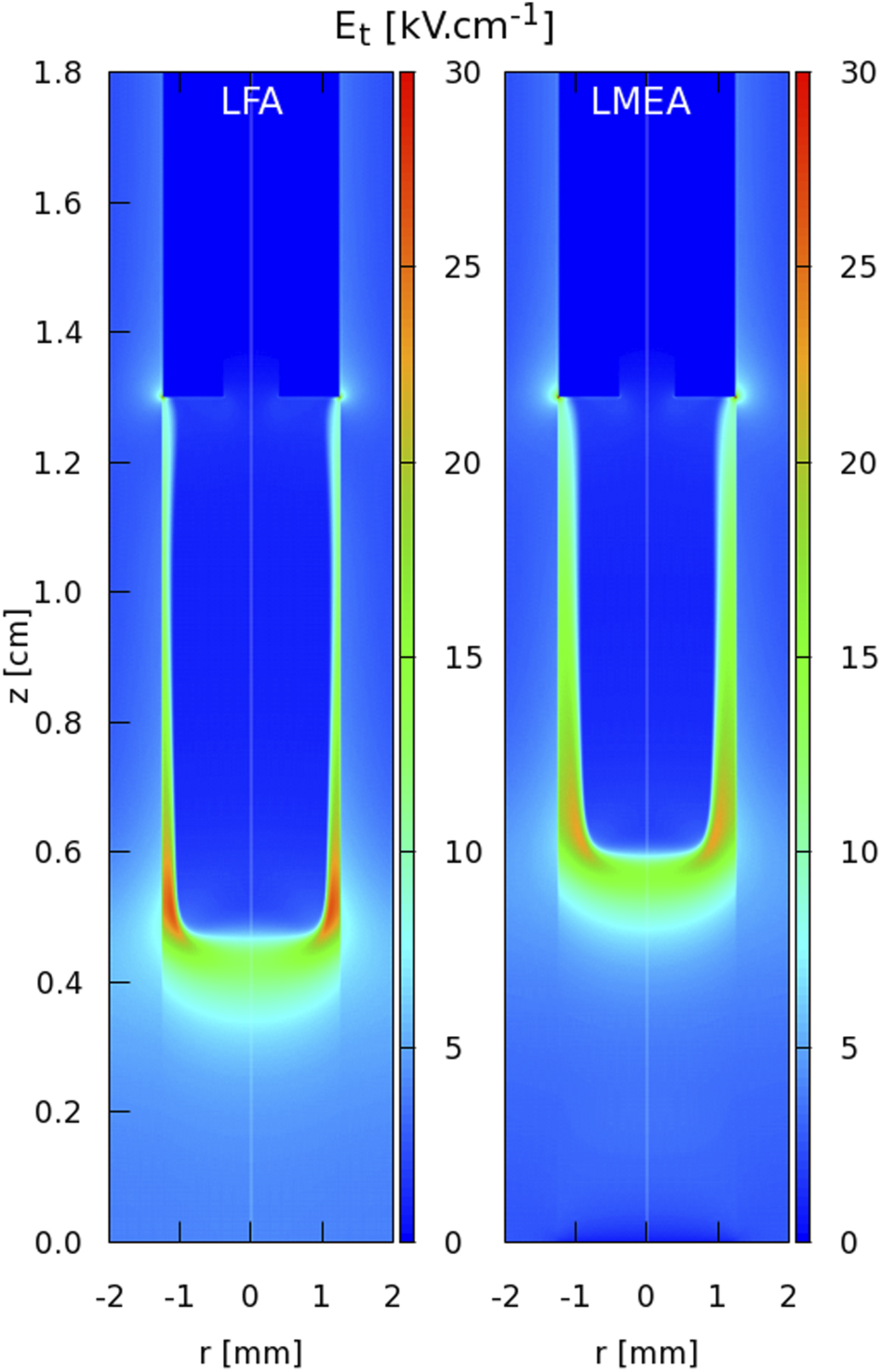
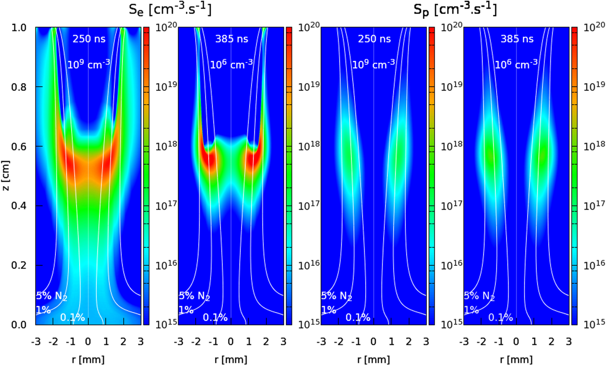
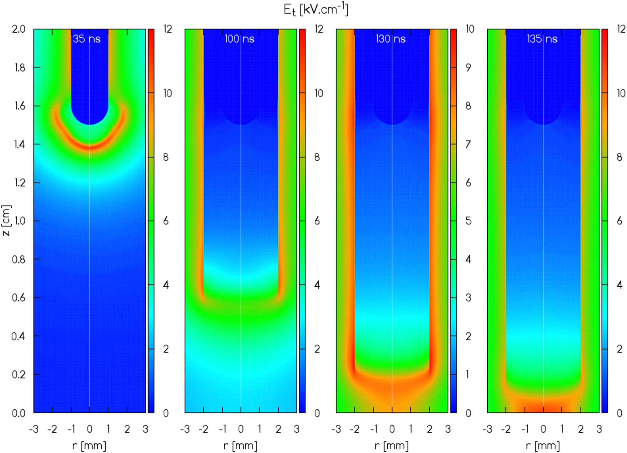
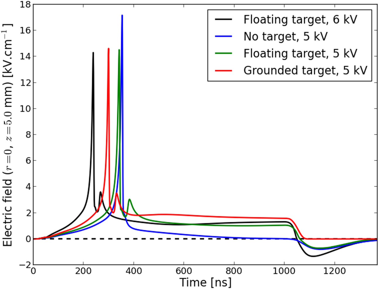
Figure 28. Temporal evolution of the electric potential in the metallic target at floating potential, from simulations and experiments, for rectangular pulses with VP = 4, 5 and 6 kV and pulse width tf = 1 and 10 μs. Reproduced from [48]. © The Author(s). Published by IOP Publishing Ltd. CC BY 4.0
Download figure:
Standard image High-resolution image
Despite the differences, both experimental and numerical results in figure 28 show a fundamental aspect of floating conductive targets: they have an electric potential close to zero at the time of discharge impact, but are highly charged at the end of the pulse, after a charging time of 100s ns or a few μs. This justifies why, in the instants after the impact on a floating conductive target, the discharge behaves approximately as with a grounded target, as visible in figures 24 and 25. The similarities include the return stroke dynamics. However, the charging dynamics also unravels important differences between floating potential and grounded targets, when considering timescales of hundreds of ns during the pulse [48, 238]. Indeed, as the target charges significantly in the mentioned timescales, the plasma–target system tends to become isopotential with floating target, while the potential gradient remains during the pulse in the grounded case. In the latter case, an electric field and the subsequent reactivity remain in the plasma channel during the pulse, leading to higher electron density and temperature (see figures 24 and 25) [48, 238]. This allows to obtain higher reactivity with grounded targets, but also opens the possibility of a potentially destructive arc transition when the current is not limited. Moreover, this feature helps to justify the higher reactive species production and higher cell inactivation when using a grounded substrate under the target in experiments [286, 290, 293]. The charging dynamics also justifies the presence of the charge relaxation event with floating potential conductive targets. As the pulse falls and an electric field is generated between the newly-grounded electrode and the highly-charged target, the charge relaxation event tends to neutralize the target (visible in figure 28) [48]. Contrarily to floating metallic targets, the electric potential of grounded metallic targets is not raised during the pulse. Hence, when the applied voltage falls to zero, the gradient of potential between the newly-grounded electrode and the plasma (and target) is higher with floating target than with grounded target. Indeed, the intensity of the charge relaxation event is proportional to the plasma potential and thus the charging of the target, which leads to a major difference between grounded and floating potential targets. Overall, these considerations confirm the importance for applications of grounding or not the target.
Finally, we should notice that, unlike the case for dielectric targets (figures 26 and 27), there is no good agreement between simulations and experiments on surface charging of metallic targets in figure 28. Indeed, the simulated electric potential rises and falls faster than in experiments, and saturates at lower values. The possible reasons for the observed disagreement have been discussed in [48]. We should notice that the simulations used to obtain the results in figure 28 have assumed field emission of electrons from the target, following a Neumann boundary condition. However, the work in [48] reports that replacing that condition by secondary electron emission through ion impact (as for the dielectric target) has little influence on the simulated temporal evolution of the electric potential. This shortcoming allows us to conclude that charge exchanges between plasmas and surfaces are not fully well known yet and deserve further investigation, as do plasma–surface sheaths. That implies that most models are not equipped to accurately describe plasma–surface interactions [216, 221].
5. Summary and outlook on future of physics of plasma jets
In most studies, plasma jets are observed to be sources of repetitive and stable ionization waves, meant for interacting with surfaces of different characteristics. As such, plasma jets provide an ideal testbed for the study of transient reproducible streamer discharge dynamics, particularly in inhomogeneous gaseous mixtures, and of plasma–surface interactions, a subject where many unknowns persist.
This topical review on the physics of plasma jets has focussed on the most fundamental physical quantities determining both discharge dynamics and plasma reactivity, such as the electric field, the mean electron energy and the electron number density. The state-of-the-art of numerical models and diagnostic techniques to describe jets and quantify these quantities has been presented, along with a benchmarking exercise between the different experimental measurements in literature. The physics of plasma jets has been described for jet systems of increasing complexity through a pedagogical approach, showing the effect of the different components of the jet system on discharge dynamics. This description has been based mostly on simulation results. It has included the ignition and propagation of helium discharges in point-to-plane geometry and within a dielectric tube, the propagation in a plume where a noble gas mixes with air, and the interaction with target surfaces. Physical phenomena imposed by different targets on the discharge, such as discharge acceleration, surface spreading, the return stroke and the charge relaxation event, have been explained and reviewed based on the state-of-the-art. Finally, this topical review has highlighted recent efforts for direct comparisons between numerical simulations and experimental measurements of the spatial and temporal distributions of electric field, mean electron energy and electron density, along with recent advances on the understanding of these quantities based on the complementarity between the different numerical and experimental techniques. With that aim, the review has focussed mostly on a specific jet configuration: a single coaxial helium kHz plasma jet powered by rectangular pulses of applied voltage, with rise-time of 10s of ns and width of 100s of ns or a few μs, without target or impacting on a solid target placed perpendicularly to the plasma jet. The comparisons have been used to shed light on the physical parameters at the discharge front, in the plasma channel during propagation and during plasma–target interaction and inside different targets.
However, not all topics of plasma jet physics have been approached in this review and there remain open questions on the physics of plasma jets and interactions with surfaces, some of which are highlighted in the following sections.
5.1. Study of memory effects
Some of the most important unknowns in plasma jet physics are memory effects, i.e. leftover elements affecting the subsequent discharges. In fact, memory effects are claimed to influence most features of dielectric barrier discharges in general [314, 315], but are poorly known. They can consist of charges remaining on surfaces, of seed electrons remaining in volume from previous discharges or of reactive species, especially long-lived metastable species, affecting the subsequent discharge dynamics. Surface charging memory effects have been recently measured and simulated for a pulsed plasma jet impacting a dielectric target and have been shown to have a direct impact on discharge dynamics [233]. That work has shown that the remainder of surface charges on the target is dependent on the applied voltage polarity and magnitude. These parameters, among others, determine the availability of free charges in the plasma after the fall of the pulse, that is crucial to neutralize the target. By following this path and using dedicated diagnostics to assess surface charges in μs and ms timescales, it would be interesting to study the dependence of leftover surface charges on plasma jet characteristics. It would be important to apply this type of investigation not only to the target, which is directly related to discharge dynamics in the plume, but also to the dielectric tube, where memory effects are likely to be more directly related to the electrode configuration and to affect discharge ignition. This study should be complemented by considering that surface properties are dependent on the studied timescales. In fact, it should be considered that the dielectric permittivity is a function of the timescale of electric field variation, and thus variable along the different phases of discharge dynamics and plasma–dielectric interaction. Furthermore, materials of weak conductivity may behave like dielectrics in short time scales but as conductive materials in long time scales.
The presence of charged and reactive species in volume in between pulses is difficult to assess both experimentally and numerically. Experimentally, because of the low density values involved in long relaxation times at atmospheric pressure. Numerically, due to the high computational times required for multidimensional plasma models to simulate long timescales and multiple pulses and due to the uncertainty in rate coefficients. However, experimental and numerical methods should be developed to pursue a more accurate knowledge of those quantities. While in electropositive gases the remaining densities of electrons and positive ions can be estimated from the electron–ion recombination coefficient (see section 2.2.3 and [181]), this is not the case when there is a high density of electronegative gases, which is typically the case in the jet plume. In that case, a more complex kinetics needs to be taken into account to estimate the remaining charges, considering also attachment, detachment and ion–ion recombination. Indeed, an accurate knowledge of the production of seed electrons may require an estimation of both the densities of negative ions remaining in between pulses and the extraction of electrons during discharge propagation, potentially via photodetachment and electric field-induced detachment [316].
5.2. Plasma–surface interactions
The sheath regions between plasmas and surfaces are regions of high density gradients, high electric fields and complex transport of charged particles. This is particularly true at high pressures, such as for atmospheric pressure discharges, in which case the sheath region can be very thin and the electric field extremely high. These are conditions where drift–diffusion LFA and LMEA approximations may lose validity, as well as the two-term EBE solution, and where several unknowns persist concerning sheath formation and development [221]. Charge exchanges between plasmas (both in the ionization front and in the plasma channel) and surfaces of different types are directly related to the sheath phenomena and are another main unknown in discharge physics. Both these phenomena are particularly difficult to assess in most atmospheric pressure streamer discharges, because of their jittering, filamentarity and stochasticity, together with the very short temporal and spatial scales involved in streamer dynamics.
In this context, plasma jets appear as an ideal source of ionization waves for the study of plasma–surface interactions. Besides being transient atmospheric pressure discharges, jet discharges are more repetitive and more stable than most streamers. These properties allow for more consistent studies of the transient dynamics of sheaths and charge exchanges at atmospheric pressure. The measurement and simulation of electric field components inside dielectric BSO targets with high temporal and spatial resolution and of the transient charging of a floating potential metallic target is a clear example of that feature. Such efforts should be pursued in order to deepen our understanding on plasma–surface interactions. In fact, the faster charging and uncharging of a floating potential metallic target in simulations than experiments (figure 28) highlights that charge transfer between plasma and solid is not yet well known. However, that experiment provides a way of testing modelling hypotheses for describing such interactions. Modelling plasma–surface interactions requires a thin mesh in the sheath region, as well as, for a particular solid wall, probabilities for sticking and backscattering of electrons, neutralization of ions and emission of electrons (through ion impact, photons or electric field). As these are very variable and usually not well known, plasma models may have to be combined with methods from solid state and surface physics [214]. These may include mesoscopic kinetic Monte Carlo and molecular dynamics simulations [220, 317], quantum kinetic methods for calculation of process probabilities [217, 218, 225, 226, 318], electric double layer models solving Boltzmann's equation for electrons and ions in the plasma and electrons and holes in solids [215, 319–321] or ab initio density functional theory simulations [214, 322, 323]. Jets can be seen as tools for assessing these theories and methods in transient atmospheric pressure conditions.
Moreover, we should notice that jet applications often employ complex targets, often of biological character, including rugosity, limited conductivity, both solid and liquid states of matter and active surface chemistry. As such, the study of plasma–surface interactions using plasma jets is expected to demand increasing levels of complexity, for which it is essential to understand the fundamentals of plasma–surface physics.
5.3. Status and perspectives on measurements of key parameters in plasma jets
Section 2.1 has highlighted recent advances in the development and application of diagnostics to assess electric field, Te and ne in plasma jets. The comparison of measurements of the peak electric field associated to the discharge front propagation, both with and without target (figure 1), has revealed that there is a relevant degree of agreement between state-of-the-art measurements, and thus a rather accurate knowledge of this quantity. Nevertheless, it would be beneficial to develop diagnostic techniques that could allow accurate measurements of the spatio-temporal distributions of electric field outside the light-emitting zone of the discharge. Currently, promising laser-based techniques such as E-FISH inherently have a low efficiency in helium because of its low polarizability, which limits its use for helium plasma jet studies.
Unlike the case for the peak electric field, the comparison of electron densities in jets (figure 2), measured in different experiments and through different diagnostics, has yielded results which vary over several orders of magnitude. Electron densities appear to be more difficult to compare from system to system, which is related not only to the different diagnostics that are used to estimate or measure them, but also to various external dependencies. Plasma jets are operated in distinct configurations (frequency, applied voltage, power, electrode geometry), which all seem to affect the reported electron density values. Rarely multiple diagnostics have been used on the same system or direct comparisons have been performed with simulations. One way to roughly compare different discharges, as discussed in section 2.1, is by measuring the current (which can vary significantly between systems, e.g. between 4–500 mA) and the propagation velocity of the ionization wave. This allows to assess whether ne measurements in different systems should be comparable. However, these quantities are not part of every reported characterization. Scaling laws for the dependency between ne and the external parameters still have to be determined and can only be found with more investigation and direct comparison between different systems.
The data on electron temperature are more scarce since they are only directly measured through Thomson scattering or estimated via other quantities like electric field or emission line intensities. The data on Te is thus less reliable since they have not been reported in great detail. Often the investigation leads to Te values specifically after the front of the ionization wave or including only the lower part of the EEDF due to limitations of the diagnostics. As a result, most reported values of Te cover the range of 0.5–3.5 eV, with some exceptions reporting 5 or 6 eV. The problem with these shortcomings is that the trends of the measured Te do not reflect the trends of the electron temperature in the discharge head. On this topic it is thus more advisable to rely on simulation results from self-consistent plasma models. Measuring electron properties in atmospheric pressure non-thermal plasmas in general is a challenge which needs to be addressed.
5.4. Status and perspectives on comparisons between experimental measurements and numerical simulations
Comparisons between experiments and simulations allow to assess the quality of models, potentially validating them, with the aim of reproducing and predicting experimental results. As such, they have the potential to increase the confidence of the scientific community not only on the knowledge and hypotheses included in models, but also on the experimental techniques under use, on the conditions for comparison and on the assessed physical quantities themselves. Nevertheless, comparing measurements and simulations may also reveal discrepancies that highlight limitations of both experimental and modelling methods. By doing so, it can provide perspectives for future improvements on both sides that should lead to an increasing understanding of the physics at play.
This review has shown that state-of-the-art LFA and LMEA models (described in section 2.2) can describe and explain several observed plasma jet physical phenomena. Moreover, by applying an LMEA model in the same conditions as experiments, measurements of position and velocity of discharge propagation (figure 18), of peak electric field on the discharge front (figure 21) and of electric field inside dielectric BSO targets impinged by the plasma (figures 26 and 27) have been reproduced. Obtaining these agreements has required to take into account the spatial and temporal averaging or uncertainty included in experimental methods. Moreover, the comparison has highlighted a disagreement between simulations and experiments on the ignition time of the discharge, which has shown the importance that a temporal shift of results can have for the quality of the comparison. The observed agreements have brought increased confidence on the experimental and numerical methods used. However, we should notice that simulation results of the same LMEA models can fail to agree with experiments on quantities such as ne and Te behind the discharge front and in the plasma channel (figures 23 and 24) and on the temporal evolution of the electrical charging of floating potential metallic targets (figure 28). The disagreement between simulations and experiments on these quantities opens the door to addressing the limitations of both state-of-the-art models and diagnostics to study plasma jets.
Experiments and simulations are expected to address more complex geometries and surface compositions than those shown in this review, and comparisons can be fundamental to reach the required understanding. Despite the highlighted advances, we can conclude that more research should be dedicated to quantitative comparisons in jets between different experimental techniques and models. Those should provide increased confidence in critical parameters for discharge dynamics of propagation, for applications in targets and in general for plasma–surface interactions. Such developments should follow verification and validation (V&V) guidelines, as those outlined recently by Fierro et al [324], including sensitivity analysis and uncertainty quantification, which requires advanced diagnostics and modelling capabilities and V&V methodologies.
5.5. Perspectives on models for plasma jets
Most simulation studies on plasma jets so far have been done using LMEA or LFA fluid models. In light of the discussion in section 5.4, some perspectives for plasma jet model improvement can be outlined:
- The development of fluid models for longer timescales (ms timescales in between pulses) and multiple pulses would allow a more accurate account of memory effects. These fluid models should account not only for ms-timescale chemistry, but also for the spatial distribution of charges in volume and on surfaces. Simulating long timescales requires, besides increasing computational capabilities, strategies to increase the calculation time-step and decrease the calculation time.
- Seed electrons are determined not only by memory effects, but also by production mechanisms such as photoionization and detachment (e.g. induced by photons or the electric field), particularly important for positive polarity discharges. As discussed in section 2.2.5, there is clearly a need to develop more accurate photoionization models for He–air mixtures taking into account the wavelength dependence of absorption and photoionization processes. It is interesting to note that the multi-group approach used for the calculation of the photoionization source term in air [211] could be used with more accurate photoionization models for He–air mixtures, when available. This would allow to calculate the photoionization source term in He–air mixtures with efficient differential methods [211].
- The description of sheaths and surface reactions is usually oversimplified in jet models. These may have to be combined with methods from solid state and surface physics, as outlined in section 5.2.
- In view of applications, more complex geometries, flow patterns and surface compositions will have to be studied. As such, a computational effort to self-consistently simulate more complex conditions in three-dimensions (3D) is important.
- Plasma jet models rely on two-term stationary homogeneous EBE solvers, that may not be accurate to describe electron kinetics in the front of transient filamentary discharges, where the electric field is compressed in a small volume (sub-millimeter scale) and evolves in ns timescales [312]. Other approaches to electron kinetics, taking into account spatial and temporal variations of electric field, should be tested in plasma jets.
- Drift–diffusion LMEA models are second-order fluid models, where the momentum conservation equation is reduced to a drift–diffusion approximation. It may be useful to test the validity of those models for the particular case of jets, in particular considering the sheaths between plasma and surfaces. Such a benchmarking exercise should include the development of more complete higher-order fluid models and of particle-in-cell/hybrid models for jets and the comparison between simulation results of different models.
5.6. Coupling of plasma jets with flows
Another area of active research is the coupling between jet discharges, gas heating and flow dynamics. This review has shown that the spatial distribution of gases in the plume is an essential feature of discharge dynamics and interaction with targets, and therefore of the yield of reactive species. However, this distribution, as well as the flow velocity, the gas temperature and the induced chemistry, can be affected by the discharge, thus constituting a mutual dependence, that can induce turbulence and instabilities. Many studies have addressed these phenomena in He and Ar plasma jets, since the first observations by Oh et al (2011) [325]. Depending on geometry, buffer gas, power conditions and timescales, many studies have concluded on the effect of gas heating affecting flow dynamics [154–156, 326], while others have indicated the importance of the EHD force to shape the flow [13, 14, 152, 153, 270, 327]. To address the interesting questions of plasma jet effects on flow and of production of chemicals for applications, it is important to consider the complex plasma chemistry taking place, including exothermal reactions, as well as the turbulent flow dynamics, along with the surface charge and charge separation remaining in the plasma in long timescales.
5.7. Tailoring of plasma jets
For the optimization of plasma jet applications, it is important to have control over setup parameters that allow to tailor the reactivity of the plasma, as well as the time and surface of plasma application on a target. This topical review has not been dedicated to that subject, although it has highlighted some effects of the tube, the electrode geometry, the spatial distribution of gases in the plume, the electrical character of the target and the polarity, magnitude, rise-time and width of the applied voltage on some of the main discharge parameters and on the charging of targets. More extensive and dedicated studies of jet control parameters have been performed, by using electrodes to apply an external electric field [39, 104, 130, 205, 271, 328–330] or by modulating the applied voltage [331–333], as reminded in the recent review by Babaeva and Naidis (2021) [143]. This is a promising subject, as applications require an increasing control over the quantities delivered by the plasma jet system.
Jets are also a tool for studying the interaction between guided ionization waves. This can be done through counter-propagating jets [144, 334–336], or by arranging a set of jet arrays, by combining tubes in parallel. This approach allows to increase the region of applied surface, and thus can be important for applications requiring uniform treatment and large areas. Jet arrays, or multijets, have been studied in the last years through experiments [75, 135, 337–343] and simulations [134, 135, 342]. These works have shown that a multiplicity of phenomena can take place when guided ionization waves interact, such as the merge or repulsion of discharges or the suppression of some discharges. These depend on the several parameters in the multijet system, including the array configuration, applied voltage, buffer gas and input flow rate, that affect the gas distribution and the electric attraction or repulsion between the discharges. Therefore, there is an extra level of complexity in the physics and application of jet arrays, when compared to single jets.
Another way of potentially increasing the surface treatment area of jets impacting targets is through the use of tilted targets, in which case the incidence of the jet on the target is not perpendicular. Indeed, the angle of incidence is another parameter of jet operation control, studied recently in [296, 344–347]. The change of angle directly affects the gas flow distribution and the electric attraction that the target inflicts on the discharge. As a result, decreasing the angle between jet and target generally results in a wider surface area covered by the plasma. This can be observed in [68, 69, 71], where significant downstream charging of a dielectric target takes place in the direction of the flow by He jet impact at 45° incidence. Together with jet arrays, tilted targets are a subject with potential for development due to the need for increasing treatment areas and to the interesting new physics at play.
Acknowledgments
The authors wish to thank the researchers who have collaborated on the study of jets: Marlous Hofmans, Enric García-Caurel, Adam Obrusník, Olivier van Rooij, Bart Klarenaar, Jean-Michel Pouvesle, Éric Robert and Thibault Darny. PV and ZB acknowledge support by Project LM2018097 funded by the Ministry of Education, Youth and Sports of the Czech Republic.
Data availability statement
The data that support the findings of this study are available upon reasonable request from the authors.