


Abstract
Glaciers distinct from the Greenland and Antarctic ice sheets are currently losing mass rapidly with direct and severe impacts on the habitability of some regions on Earth as glacier meltwater contributes to sea-level rise and alters regional water resources in arid regions. In this review, we present the different techniques developed during the last two decades to measure glacier mass change from space: digital elevation model (DEM) differencing from stereo-imagery and synthetic aperture radar interferometry, laser and radar altimetry and space gravimetry. We illustrate their respective strengths and weaknesses to survey the mass change of a large Arctic ice body, the Vatnajökull Ice Cap (Iceland) and for the steep glaciers of the Everest area (Himalaya). For entire regions, mass change estimates sometimes disagree when a similar technique is applied by different research groups. At global scale, these discrepancies result in mass change estimates varying by 20%–30%. Our review confirms the need for more thorough inter-comparison studies to understand the origin of these differences and to better constrain regional to global glacier mass changes and, ultimately, past and future glacier contribution to sea-level rise.
Export citation and abstract BibTeX RIS
1. Introduction
Glaciers are an iconic symbol of climate change (Oerlemans 2005). Their geometry responds to changes in temperature and precipitation at yearly to decadal time scales in ways that are easily perceived by humans. Their rapid present-day shrinkage has direct, and sometimes severe, consequences on some inhabited areas on Earth as their meltwater contributes significantly to rising sea level (Meier 1984, Cazenave et al 2018, Frederikse et al 2020) and alters regional water resources in arid regions (Huss and Hock 2018, Pritchard 2019). Glacier retreat also has a distinct effect on biodiversity, tourism and glacier hazards (Haeberli and Whiteman 2015, Cauvy-Fraunié and Dangles 2019, Salim et al 2021).
This review deals with all glaciers on Earth, i.e. the more than 200 000 ice bodies disconnected from or weakly connected to the Greenland and Antarctic ice sheets (Pfeffer et al 2014, RGI Consortium 2017). Their cumulative size (∼700 000 km2) is rather modest compared to the two giant ice sheets. Their overall volume is such that, if they were to melt entirely, sea level would rise by about 30 cm (Farinotti et al 2019, Millan et al 2022), which is one to two orders of magnitude smaller than the same quantity for the two ice sheets. However, being highly sensitive to climate fluctuations (Oerlemans 2001, Cuffey and Paterson 2010), even a small climate imbalance leads to rapid mass change. Glacier mass change remains one of the least-constrained components of the global water cycle, and was identified as a critical research gap in the 2019 Intergovernmental Panel on Climate Change (IPCC) Special Report on the Ocean and Cryosphere in a Changing Climate (Portner et al 2019).
The glacier-wide mass balance rate is a key variable to characterise the state of health of glaciers, their contribution to river runoff and sea level rise (Marzeion et al 2014, Zemp et al 2019, Hugonnet et al 2021). It is defined as the change of mass of an entire glacier (or an entire glacierised region) and expressed in gigatons per year (Gt yr−1 = total mass balance in this review). For improved comparability between glaciers or regions of contrasting sizes, this quantity is often divided by the glacierised area and is expressed as metre water equivalent per year (m w.e. yr−1 = specific mass balance), which is equivalent to the water layer gained or lost on average during one year (Cogley et al 2011).
Traditionally, and during most of the 20th century, glacier mass balance has been derived from pointwise field observations performed on a few dozen glaciers by repeatedly measuring the melt at ablation stakes and the snow accumulation from pits or cores in the accumulation area (Thibert et al 2008, Zemp et al 2015). These in situ measurements of the surface mass balance (SMB) were sometimes complemented with repeat airborne photogrammetric flights to measure multi-year volume change and validate/calibrate the field measurements (Zemp et al 2013, Andreassen et al 2016). Global mass change estimates were then derived by extrapolating these few tens of measurements to the entire glacier sample (Meier 1984, Kaser et al 2006), leading to large uncertainties or even biased estimates (Gardner et al 2013). Since the start of the 21st century, the launch of novel spaceborne sensors has fostered the emergence of remote sensing methods to measure glacier mass changes at local, regional and global scales (Bamber and Rivera 2007, IGOS 2007, Marzeion et al 2017, Haeberli et al 2021, Taylor et al 2021).
This review aims at presenting and comparing these modern satellite-based techniques (figure 1), i.e. digital elevation model (DEM) differencing (section 3), repeat radar (section 4) and laser (section 5) altimetry, and gravimetry (section 6). This review does not address the input/output (or component) method. This method estimates the glacier mass change as the difference between the SMB and the ice discharge (Noël et al 2018). In this method, the only mass balance component effectively measured from space is the frontal ablation, which in general is a modest part of the overall mass budget (Błaszczyk et al 2009, McNabb et al 2015, Van Wychen et al 2016, Kochtitzky et al 2022). The input/output method is thus too heavily based on in situ measurements or models to estimate the SMB (Bamber et al 2018) to be considered in the present review.
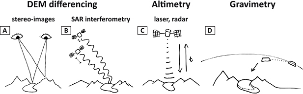
Figure 1. Sketch of the main techniques used to estimate glacier mass change from space. DEM differencing and altimetry (A)–(C) first determine glacier volume changes through repeat measurement of the glacier elevations. The sources of elevation data are usually DEMs, commonly derived from (A) satellite stereo images, where two satellites 'see' the terrain in 3D just as humans do with their two eyes, or (B) SAR interferometry, which reconstructs the surface terrain from the phase difference of the recorded microwave signal at two SAR satellites that fly very close together. Other sources or point/profile-based elevation data are (C) radar and laser altimetry, which determines the surface elevation directly under the satellite by means of the two-way travel time of a radar/laser pulse. (D) Satellite gravimetry is used to detect mass changes directly: two satellites on the same orbit are connected with a ranging system that detects acceleration/deceleration of the satellites relative to each other caused by changes in the gravimetric force. These changes include, among others, glacier mass change between different satellite overpasses. Source of A, B and C: Treichler (2017). Reproduced with permission from Treichler (2017).
Download figure:
Standard image High-resolution imageBecause all the satellite-based techniques rely at some point on the availability of a global inventory of glacier outlines, the review starts with a presentation of the state-of-the-art on glacier mapping from space (section 2). In a final section (section 7), we compare the ability of the different techniques to depict the elevation changes and mass balance of a large Arctic ice cap (Vatnajökull, Iceland), steep glaciers in the Everest area and discuss their respective strengths and weaknesses with a regionally-differentiated perspective. Our goal is not an exhaustive overview of the Earth observation satellite missions used in glaciology, i.e. we only consider the satellite missions that have been used specifically in glacier mass balance studies (figure 2).
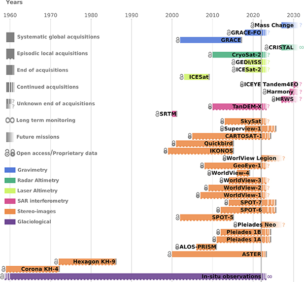
Figure 2. Overview of the lifetime of the main satellite missions used in glacier mass balance studies (as of October 2022). The colours distinguish different types of satellite sensors. The '?' is used when the decommission date is not known and '∞' for long term (i.e. operational) monitoring without a specific end date. A distinction is also made between missions that provide systematic 'global' coverage and others that make 'local' acquisitions on demand. 'Open access' missions are those for which the data are fully open access to all users. Conversely, 'proprietary' is used for commercial missions or missions for which the access is limited to certain users, for example upon acceptance of a research proposal. The list of future missions is not exhaustive but aims at illustrating a potential gaps for certain categories of data (notably, laser altimetry and 'open access' stereo-images with global coverage).
Download figure:
Standard image High-resolution image2. Importance of an accurate glacier inventory
The main purpose of a glacier inventory is to characterise the area covered by glaciers (i.e. where are they?) and the volume or mass of ice they store (i.e. how much ice do they contain?). Whereas glacier outlines define the region covered by glacier ice, glacier area distribution with elevation (i.e. glacier hypsometry) is of key importance for numerical modelling of glacier evolution and for hydrological models. Glacier volume is derived from a range of methods and needed for water resources assessment as well as calculation of glacier contribution to sea-level rise. With glacier changes (in length, area and volume) being widely accepted as key indicators of climate change (Oerlemans 2005, Bojinski et al 2014, Trewin et al 2021), a glacier inventory also provides a base for change assessment when mapped outlines are available for at least two points in time. Related assessments over longer time periods also provide information about glacier health. For example, glaciers losing area at their highest elevations are in a strong disequilibrium with climate and will ultimately disappear (Pelto 2010, Carturan et al 2020).
When glacier outlines are combined with a DEM, a wide range of glacier-specific topographic characteristics can be derived (Kienholz et al 2015), which allows calculating further metrics to describe a glacier (Haeberli and Hoelzle 1995). For example, glacier median (or mean) elevation is widely used as a proxy for the equilibrium line altitude (ELA) for a glacier with a zero mass balance (Braithwaite and Raper 2009). When this so-called balanced-budget ELA0 is known, a rough climatic classification of glaciers can be derived (Ohmura et al 1992) which opens a wide range of further calculations, including details about precipitation in high mountains regions (Sakai et al 2015). And, most importantly, glacier outlines spatially constrain glacier-specific calculations such as elevation changes, flow velocities and debris-covered fractions (Scherler et al 2018). For the former two, glacier outlines also constrain where 'off glacier' terrain is. These stable regions can be used for several steps in the data processing (e.g. DEM co-registration) and for the uncertainty assessment (e.g. Nuth and Kääb 2011). In short, glacier outlines are required for nearly all glacier-related calculations (Kargel et al 2005). But how are glacier outlines created?
Nowadays, scientists use inventories readily available, most frequently from the Global Land Ice Measurements from Space (GLIMS) glacier database (which is multi-temporal) or the Randolph Glacier Inventory (RGI), which provides a single snapshot of glacier extents and is available in a globally near complete version since 2011 (Pfeffer et al 2014). Since then, the RGI has been continuously improved and is now available in its version 6 (RGI Consortium 2017). Outlines available in the GLIMS database and from the RGI have been freely provided by the scientific community on a voluntary basis as an outcome or by-product of diverse research projects. This means that updating and filling of the database is slow and is so far uncoordinated. Today, a working group 16 of the International Association of Cryospheric Sciences (IACS) is coordinating glacier data compilation and redistribution. The group also prepares the release of RGI version 7.
As glacier outlines are mostly derived from optical satellite images, the opening of the Landsat archive in 2008 (Wulder et al
2012), with free access to orthorectified imagery, started a new era in global glacier mapping and change assessment. Semi-automated mapping of glaciers from multi-spectral satellite data using previously developed methods (Hall et al
1987, Bayr et al
1994, Paul et al
2002) were applied to large samples of glaciers all over the world (Bolch et al
2010, Frey et al
2012, Guo et al
2015). The most popular method is based on a simple red (noted R, or near infrared)/short wave infrared (noted SWIR) band ratio that increases contrast between ice and snow as their reflection is close to zero in the SWIR band. This allows distinguishing snow and ice from all other terrains or clouds with a simple threshold th applied to the ratio image, e.g.  .
.
To achieve the best possible results, the threshold value (e.g. th= 1.5) has to be selected and optimised manually for individual regions and scenes, in general balancing the inclusion of dark ice in cast shadow and excluding bare rock (Paul et al 2016). The resulting binary image is transformed to polygons using raster to vector conversion (figure 3). Remaining omission (ice hidden by clouds or debris cover) and commission errors (water, bare rock, seasonal snow, lake and river ice) have to be manually corrected during post-processing. In regions with many debris-covered glaciers, this last step is very laborious and time consuming (Racoviteanu et al 2022). Debris cover on glaciers is thus the bottleneck of global glacier mapping efforts and hinders rapid and easy updates of the global datasets with its >200 000 glaciers. Once glacier outlines with debris cover are mapped, the extent of debris cover can be determined as a residual from automated clean ice mapping (Scherler et al 2018, Herreid and Pellicciotti 2020). Other problematic factors are remaining seasonal snow and clouds hiding the glacier perimeter. Both require that only the most appropriate scenes are selected from the archives for glacier mapping. In maritime regions with abundant clouds and late lying seasonal snow, high-quality glacier extents can thus only be mapped occasionally, typically every 5–10 years. This has improved a bit with the more frequent observations from Sentinel-2 (at least every five days, even more often towards higher latitudes), as the chance for cloud-free images acquired at the end of the ablation period has considerably increased.

Figure 3. Glacier mapping with the band ratio method applied to Landsat Thematic Mapper (TM) images of Unteraar (upper glacier in the image) and Oberaar (the one in the centre) glaciers in the Bernese Alps, Switzerland. (A) TM band 3 (red), (B) TM band 5 (shortwave infrared), (C) band ratio TM3/TM5, (D) the resulting binary glacier map after applying a threshold to (C), (E) glacier outlines after raster—vector conversion of (D), and (F) overlay of the outlines seen in (E) in black with manually corrected extents in yellow, adding the unmapped glacier area under debris cover. The background image in (F) is a false-colour composite with TM bands 5, 4, and 3 as red, green and blue, showing ice and snow in light blue, bare rock in pink to brown and vegetation in green to yellow. Landsat-5 image courtesy of the U.S. Geological Survey. Source: glovis.usgs.gov.
Download figure:
Standard image High-resolution imageAn important issue when using glacier outlines for elevation change calculation is good spatial and temporal matches. The outlines should refer to the larger glacier extents, e.g. for retreating glaciers the date of the first DEM. As many DEM differencing studies use the Shuttle Radar Topography Mission (SRTM) DEM (February 2000) or the first Advanced Spaceborne Thermal Emission and reflection Radiometer (ASTER) DEMs (from 2000 or 2001) as a starting point, and because the vast majority of glaciers are shrinking worldwide (Zemp et al 2015), glacier outlines derived from satellite images acquired around the year 2000 are preferable. Most outlines in RGI version 6 have been acquired between 2000 and 2010, but several regions only offer much older (1960s to 1980s) or more recent extents. It might thus be required to correct these manually. A manual correction is also needed in the case of surging glaciers so that the rapid volume gain at their advancing terminus is not missed (Berthier and Brun 2019). A poor spatial match can arise when the DEM used for orthorectification of the satellite images is different from—or of a lesser quality than—the DEMs used to obtain elevation changes (Kääb et al 2016). The related horizontal shifts cannot easily be corrected as they are non-systematic.
The specific mass balance is computed as the total mass balance divided by the mean glacier area over the study period (Cogley et al 2011, Fischer et al 2015). Thus, in principle, two sets of glacier outlines should be available, one at the start and one at the end of the study period. Practically, this is often not the case, especially for studies with a regional or global scope that mostly use the RGI (Zemp et al 2019, Hugonnet et al 2021). Uncertainties due to the lack of a repeat inventory or too low quality of some outlines in the RGI can be assessed in regions where state-of-the-art and repeat inventories are available (e.g. section 7 in the supplementary material of Dussaillant et al (2019)). As glacier area loss is fast, sometimes over 1% per year (Paul et al 2020), repeat regional and global inventories are needed.
Finally, differences in how to interpret/identify which parts belong to a glacier can have an impact on mass balance estimates. Again, debris-covered glacier parts introduce the largest uncertainty in interpretation (Paul et al 2013) and can, moreover, easily be confused with rock glaciers. These might look morphologically very similar and the transition to a debris-covered glacier can be gradual as in cold/dry climates some rock glaciers might have developed from heavily debris-covered glaciers (Janke et al 2015). Depending on which glacier extent is used and how strong the changes are in the uncertain glacier zone, clear differences in the specific mass balance (and to a lesser extent the total mass balance) can occur across different studies (Ferri et al 2020). This needs to be homogenised, but until then, a precise description of the glacier inventory used (and the modifications applied) is required to allow intercomparison of results from different studies.
3. Differencing of DEMs
The comparison of multi-temporal DEMs, often referred to as the geodetic method, has been used for decades to build maps of glacier elevation changes (dh). Division by the time separation between the two surveys gives elevation change rates (dh/dt) that can then be converted to mass balance using an assumption on the density of the material gained or lost. Initially applied to DEMs derived from maps (e.g. Adalgeirsdóttir et al 1998, Nuth et al 2007, Palsson et al 2012), aerial photographs (Finsterwalder 1954, Thibert et al 2008) and more recently to airborne lidar data (Echelmeyer et al 1996, Abermann et al 2010), the technique has been used since the early 2000s with satellite DEMs, often in conjunction with older maps (Rignot et al 2003, Berthier et al 2004, Kääb 2008). We first describe the principle of the method (3.1) before presenting the two main sources of satellite DEMs, optical stereo-imagery (3.2) and interferometric SAR data (3.3).
3.1. Principle
The method consists in coregistering and then differencing two DEMs, i.e. two grids representing the elevation of the glacier surface at two epochs in time. Since 2012, the method has also been modified to tackle time series of DEMs, either using a simple linear regression through the elevation time series (Nuimura et al 2012, Willis et al 2012) or using a more advanced statistical framework to resolve non linearities in the glacier elevation change signal (Hugonnet et al 2021).
A key preprocessing step is the relative adjustment of the different DEMs on the stable terrain surrounding the glaciers. The compared DEMs must share the same map projection and, importantly, be referenced to the same elevation datum (geoid or ellipsoid, see https://doi.org/10.5194/tc-2021-197-CC1). A first and mandatory step is to correct the horizontal and vertical shifts between the DEMs using, for example, the coregistration method from Nuth and Kääb (2011). In the case of spy satellite images (presented below), an affine transformation (rotation, scaling) or more complex non-linear shifts may have to be corrected beforehand (Maurer and Rupper 2015, Dehecq et al 2020). After applying this translation vector, some sensor-specific artefacts may remain and need to be modelled to approach an unbiased elevation change estimate (Nuth and Kääb 2011). For example, undulations in the DEMs in the along-track direction, related to the jitter of the platform, are common in optical imagery (Girod et al 2017). In other cases, tilts or along/cross track biases between the DEMs have to be corrected (Shean et al 2016). If DEMs of different original resolutions are compared, some biases related to the terrain morphology may also persist. Terrain curvature proved to be a good proxy for correcting the latter biases (Gardelle et al 2012). After relative adjustment, DEMs can be subtracted (or processed as a time series) to map elevation changes.
There are two final hurdles before obtaining the glacier-wide total mass balance, two issues which are shared with the altimetry-based estimates discussed in sections 4 and 5 of this review. (a) The first one is the need to fill in data gaps in the map of elevation changes. These gaps are often distributed unevenly and thus, if not filled properly, may lead to biased estimates. For example, native stereo sensors from the late 1990s or early 2000s such as ASTER or Satellite Pour l'Observation de la Terre (SPOT) 5 acquired imagery using eight-bit sensors (for which images are made of 28, i.e. 256 digital numbers) leading to poor radiometric dynamics in the bright, textureless accumulation area of glaciers, and hence a concentration of data gaps. As these upper regions often experience attenuated elevation changes than the lower reaches (Schwitter and Raymond 1993, Belart et al 2019), filling these gaps with a glacier-wide average value would bias the mass balance estimate. Several approaches have been developed to fill data gaps (Seehaus et al 2020), one of the best performing and robust being the local hypsometric approach that exploits the fact that elevation changes are often correlated with altitude (McNabb et al 2019). (b) The second hurdle is the conversion of the volume change to mass change. This requires an estimate of the density conversion factor (Cuffey and Paterson 2010). Here again, various strategies have been used. Assuming an unchanged vertical density profile (the so-called Sorge's law), many studies (e.g. Bader 1954, Arendt et al 2002) used a single ice density (900 kg m−3). Others (e.g. Haag et al 2004) have favoured separating the ablation area (where ice is lost at a density of 900 kg m−3) and accumulation area, where they used an average density for the firn (often 500–600 kg m3), assuming, implicitly, a change in the vertical density profile. Huss (2013) used a firn densification model calibrated with in situ measurements of firn density to show that a single density of 850 ± 60 kg m−3 was a good compromise for glacier-wide estimates over a measurement period longer than five years (and ideally longer). Improvements in this volume to mass conversion are still needed as it remains the largest source of errors in a recent estimate of global glacier mass change (Hugonnet et al 2021).
Due to these uncertainties in the volume to mass conversion and the precision of the elevation change measurements, DEM differencing is typically applied over periods of 5–10 years, although dense time series of DEMs can also allow exploring short term, seasonal elevation changes (Seehaus et al 2015, Belart et al 2017, Beraud et al 2022). The temporal resolution and timeliness of the geodetic mass balance record can be improved with ancillary data such as in situ mass balance measurements (Zemp et al 2019, 2020) or snow line satellite observations (Davaze et al 2020, Barandun et al 2021).
3.2. DEM from optical stereo-imagery
The principle of DEM generation from a stereoscopic pair is simple and has been used for decades by national mapping agencies to chart the Earth's land topography using overlapping aerial photographs. It consists of estimating the distortions (also called the parallax) between pair, triplet or more images acquired from different viewpoints. If the acquisition geometry (position, pointing angles) of the images are known, the parallax can be converted to terrain elevation. For an historical background, the reader is referred to a review (Toutin 2001) describing the early days of DEM generation from optical satellite images.
The main drawback of optical (visible or near infra-red) images, compared to radar data, is that they are weather dependent. No DEM can be derived during the (polar) night or when clouds obscure the Earth's surface. Another notorious limitation is that DEMs derived from these images often concentrate data gaps and exhibit more noise in the snow-covered accumulation areas. We will see below that this is however not true anymore for modern stereo-imagery.
In the following, we distinguished two generations of stereo sensors depending on their resolution. We focus on the sensors that have been most used for estimating glacier elevation changes and do not aim at an exhaustive overview.
3.2.1. Stereo sensors with decametric (5–15 m) resolution.
Early satellite multispectral sensors (Landsat, SPOT) did not have built-in stereo capabilities. However, the SPOT1-4 satellites could point across track so that stereo pairs were assembled on-demand using images acquired a few days or weeks apart from different orbits. DEMs have been derived from such image pairs (AlRousan et al 1997), including for alpine glacier tongues in the 1990s or early 2000s (Berthier et al 2004). A severe limitation of these across-track stereo acquisitions was the loss of visual similarities between images acquired several days apart, the increased risks of clouds and the fact that glacier surface displacement between the two acquisitions could bias the measurement of the parallax. In the SPOT1-4 image catalogue, the number of such opportunistic stereo pairs is limited.
The sparse availability of stereo pairs from civil satellites before 2000 can be compensated by the declassification of spy satellite images from the 1960s, 1970s and 1980s acquired by missions such as Corona and Hexagon (Surazakov and Aizen 2010). They provide very useful data to measure multi-decadal glacier mass balance and put the recent changes (i.e. post-2000) in a longer perspective as done for the Himalaya and the Tibetan Plateau (Holzer et al 2015, Zhou et al 2018, Maurer et al 2019). The recent development of open-source tools to calculate DEMs from these images (Belart et al 2019, Dehecq et al 2020, Ghuffar et al 2022) should further increase their use in the future.
In the civil domain, native stereo capabilities emerged in the early 2000s with the ASTER sensor on board the Terra satellite (Hirano et al 2003) and the high resolution stereoscopic (HRS) instrument on board SPOT5 (Gleyzes et al 2012). Both sensors are made of two telescopes, one pointing forward (or towards the nadir for ASTER) and the other backward. Stereo pairs are thus systematically acquired along track within a few tens of seconds, resulting in a large archive of scenes suitable for DEM generation. Members of the GLIMS project were involved in the ASTER Science team and ensured that glaciers were among the priority targets for ASTER (Raup et al 2000). Importantly, the GLIMS team also tuned the gain setting to avoid saturation of the images over the bright snow-covered areas. Numerous glaciological studies exploited the ASTER stereo-capabilities following some promising early results (Kääb 2002, Kargel et al 2014). Since April 2016, ASTER images have been freely available which boosted their use by the scientific community. As of writing, ASTER is still acquiring stereo pairs but the end of the mission is planned for late 2023 and, unfortunately, ASTER will not be replaced.
The SPOT5-HRS archive (2002–2015) has been publicly opened recently (June 2021) as part of the SPOT World Heritage program (https://regards.cnes.fr/user/swh/) from the French Space Agency, CNES. Before that, access to the images was restricted to the French mapping agency and the French defence. Only during the international polar year, 2007–2009, a dedicated image acquisition program took place over the polar regions. The SPIRIT (Spot5 stereoscopic survey of Polar Ice: Reference Images & Topographies) initiative distributed 40 m DEMs and 5 m ortho-images of glaciers and ice sheet margins to the scientific communities (Korona et al 2009). The SPOT5-HRS archive is large and almost unexploited. Outside the SPIRIT period, this mission did not benefit from a fine gain setting for glacier and ice sheets (contrary to ASTER) so that many images in the catalogue may be too saturated for DEM generation.
The panchromatic remote-sensing instrument for stereo mapping (PRISM), onboard the ALOS satellite, also has native stereo capabilities (triplet of images acquired along track) together with a promising 2.5 m resolution and a 60 km swath. SPOT6 and SPOT7 have a similar swath but even higher resolution (1.5 m). DEMs derived from PRISM or SPOT6/7 have been less used by the glaciological community (Lamsal et al 2011, Ragettli et al 2016, Berthier and Brun 2019), likely because data access is not as straightforward as for ASTER. The same also applies to Cartosat-1 (Pieczonka et al 2011).
Various software has been used to generate DEMs from the stereo-pairs. Up to a few years ago, most of the processing was done using commercial software such as PCI Geomatica (Toutin 2001) or ERDAS (Bolch et al 2008). Recently, open-source tools such as MicMac, SETSM or ASP have been developed to process high resolution images (Noh and Howat 2015, Beyer et al 2018, Rupnik et al 2018) and were also adapted to medium resolution images (Girod et al 2017, Shean et al 2020).
3.2.2. Stereo sensor with metric to submetric resolution.
In the second part of the 2000s and during the 2010s, a novel generation of high resolution satellites was launched, including Worldview (WV, DigitalGlobe, now Maxar) and Pléiades (CNES and Airbus Defence & Space, DS). These satellites have a sub-metre resolution and are characterised by a high agility so that stereo pairs (or triplet) can be formed from along-track acquisitions a few tens of seconds apart. Two characteristics have dramatically increased the quality of the DEMs that can be derived from these modern sensors over snow and ice. First, the radiometric depth has evolved from 8 bits for ASTER, SPOT1-5 (and others) to 11 or 12 bits (2048 or 4096 digital numbers) for WV1-4 and Pléiades (and SPOT6/7). Second, the sub-metre resolution means that fine scale features of the terrain can be resolved. Both characteristics lead to images with a lot of contrast even in the snow-covered accumulation areas and almost no saturation. This implies that (a) the entire archives are useful for glaciology (without any special gain setting) and (b) the correlation between the stereo-pair works efficiently so that almost complete DEMs can be constructed even over ice sheets (Shean et al 2016, Howat et al 2019) or the glacier accumulation areas (Berthier et al 2014). The higher spatial resolution and the good knowledge of the orbits also results in a higher vertical precision of the DEMs. The improvement in resolution and precision between ASTER and Pléiades is illustrated for the Meighen Ice Cap (figure 4). As a rule of thumb, the vertical DEM precision is on the order of the image resolution.
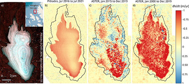
Figure 4. (A) False colour (near-infrared) image of Meighen Ice cap, Canadian Archipelago (Burgess and Danielson 2022), from a Pléiades scene acquired in July 2016 (© CNES 2016, distribution Airbus DS). (B)–(D): Rate of elevation change (dh/dt in m yr−1) for the Meighen Ice Cap (RGI60-03.00691) during five years periods, from two Pléiades stereo-pairs acquired 29 July 2016 and 19 July 2021 ((B), this study), from all ASTER stereo-images acquired (C) between 1 January 2015 and 31 December 2019 (Hugonnet et al 2021) and (D) during the 20 year period from 1 January 2000 to 31 December 2019 (Hugonnet et al 2021). The black polygon is the RGIv6 outline, derived from 1999–2003 imagery according to the RGI handbook, although these elevation change maps suggest that the outlines were derived from older imagery. Note the sharply reduced noise level from very high resolution 12-bit Pléiades stereo-imagery compared to ASTER (8-bit images) and also the need for an updated glacier inventory to properly estimate the specific mass balance of this ice cap. Credit: Pléiades © CNES 2016, distribution Airbus DS.
Download figure:
Standard image High-resolution imageThe sub-metre resolution is obtained at the cost of relatively narrow swaths (∼10–20 km) compared to, for example, ASTER (60 km) or SPOT-HRS (120 km). This means that several images, often acquired over the course of several days or weeks, need to be mosaicked to cover a large ice cap or an entire mountain range. Another drawback is that these sensors are commercial, which complicates data accessibility for the scientific community. They mostly acquire images on-demand and contrary to ASTER, they do not continuously build a vast archive of stereo images. Exceptions to this rule are the numerous, time-stamped WV DEMs freely available in the Arctic (ArcticDEM, Porter et al 2018), Antarctic (REMA DEMs, Howat et al 2019) and in High Mountain Asia (Shean et al 2020). Dedicated acquisition campaigns are also performed by the French Space Agency (CNES) through the Pléiades Glacier Observatory 17 .
3.2.3. Future missions with stereo capabilities.
Several space agencies are on the way or have projects to launch more satellites with improved stereo capabilities such as Pléiades Neo from Airbus DS or WorldView Legion for Maxar. In 2024, CNES and Airbus DS will launch the CO3D constellation 18 with the main goal to build a global high resolution DEM. However, none of these missions is open-access and scientifically driven.
A game changer would be a future satellite stereo mission with a high resolution (on the order of 1–2 m), capable of covering a large extent of terrain in a short period of time and continuously acquiring freely available images. Such a concept, currently named Sentinel-HR 19 , is being promoted by scientists from several disciplines and explored further by the French Space Agency (Iliopoulos et al 2022).
3.3. DEM from radar imagery
Spatially-distributed surface elevation information can also be gained from single-pass across-track interferometric (InSAR) data. In this case, a radar system with spatial separation (baseline) between transmitter and receiver is required for the data acquisition, with one antenna transmitting and both receiving the complex SAR signal. This so-called bistatic instrument configuration enables the generation of high quality interferograms that are not affected by temporal decorrelation and ice motion and with reduced atmospheric effects (Bamler and Hartl 1998, Rosen et al 2000).
The cross-track technique is based on the evaluation of phase differences measured by the two SAR antennae. While in a single SAR image the location of each surface point is reduced to the range distance, this technique is a means to measure also the radar look angle allowing to recover the point's location in space. The interferometric phase difference of every pixel is used to determine the difference between the two range distances to the SAR antennae which in turn can be considered a measure of the radar look angle (Bamler and Hartl 1998). A sensitivity measure of the interferometrically derived elevation is the height resulting from a phase change of one fringe (2π) which represents one ambiguity cycle. This height of ambiguity is inversely proportional to the perpendicular component of the baseline, the effective baseline. A larger effective baseline leads to a dense fringe pattern, hence higher precision but also more difficult unwrapping. Conversely, a smaller baseline leads to a noisier DEM but a more robust unwrapping. Additionally, the radar wavelength also has a directly proportional influence, a low frequency SAR (e.g. L-band, 1.25 GHz) generates larger heights of ambiguities and thus less sensitive DEMs than a C- or X-band SAR system (5.3 GHz and 9.6 GHz, respectively).
3.3.1. Elevation data from spaceborne bistatic InSAR systems.
To date, two spaceborne InSAR missions have been launched with the primary objective of measuring Earth's topography.
The first single-pass interferometer, SRTM, was flown from 11 to 22 February 2000 and was a unique experiment with two antennae on the same platform, the second antenna located on the end of a 60 m long mast (Farr et al 2007). Thus, the SAR data were acquired with a known, constant baseline during the mission. The coverage of the resulting DEM is, however, principally limited to a latitude range from 56°S to 60°N due to the inclined orbit of the Space Shuttle and its mapping geometry. The good vertical accuracy (better than 9 m) and the short temporal baseline provided a snapshot of the glacierised areas within these latitudes. The SRTM C-band DEM (processed by the National Aeronautics and Space Administration, NASA), obtained by combining overlapping ascending and descending strip data, has been widely used due to its completeness and it is available for free download in various versions, the latest being released in February 2020 by the Land Processes Distributed Active Archive Center (LPDAAC). The SRTM X-band DEM, processed by the German Aerospace Center (DLR), is also available but has wide gaps due to the narrower swath and is therefore less used.
The second mission, TanDEM-X (TerraSAR-X add-on for digital elevation measurements), is currently in orbit and consists of the coordinated operation of two almost identical satellites—TerraSAR-X (TSX) and TanDEM-X (TDX), the latter named similarly as the mission—flying in close helix formation (Krieger et al 2007). The mission has been operational since December 2010. The primary objective of the TanDEM-X mission is the generation of a worldwide, consistent, timely, and high precision DEM which was released in 2018 (Wessel et al 2018). Operational data acquisition for DEM generation is performed using the bistatic InSAR stripmap mode (30 km swath width): either the TSX or TDX satellite is used as a transmitter to illuminate a common radar footprint on the Earth's surface. The scattered signal is then recorded by both satellites simultaneously. Both satellites act as a large single-pass radar interferometer with the opportunity for flexible baseline selection. Prerequisites for bistatic operation of this fully active system are the pulse repetition frequency synchronisation and the relative phase referencing between the two satellites.
The global DEM product of the TanDEM-X mission (DLR-EOC 2018), whose performances are analysed in Rizzoli et al (2017) and Wessel et al (2018), is the result of the combination of four years (from 12 December 2010 to 16 January 2015) of bistatic data acquisitions with different baselines and geometries. In order to compensate residual offsets and tilts after the interferometric processing, this product is calibrated to selected ICESat points except in Greenland and Antarctica. Hence the global TanDEM-X DEM is not suitable for the derivation of surface elevation changes, but rather as a reference DEM for various purposes. Instead, individual bistatic TanDEM-X acquisitions can be processed to timestamped DEMs and used to generate time series of surface elevations at yearly or multiyear intervals over regions with high mass losses (Abdel Jaber et al 2019, Braun et al 2019). Compared to early volume change assessments for which DEMs from different sensors were combined, the TanDEM-X single-pass interferometer offers significant improvement in terms of spatial resolution (typically 5–10 m) and vertical accuracy. Typically, elevation changes are measured within ±1 m if ice free areas are available for proper adjustment of the DEMs.
The map of surface elevation change rate over the Western Vatnajökull Ice Cap (Iceland) obtained from two TanDEM-X 30 km-wide strips is shown in figure 5. The 2012 DEM is composed of ascending acquisitions in August (western strip) and June (eastern strip). The second coverage was achieved with ascending acquisitions in winter 2016, with the western strip from December and the eastern from November. The DEMs were vertically coregistered over ice free areas. The decrease in elevation from 2012 to 2016 can be clearly observed at the outlet glacier termini, while higher on the ice cap the surface elevation is almost constant or slightly increases. The obvious large spot of surface lowering in the Northwest of the ice cap is caused by the Bárðarbunga caldera collapse in 2014/2015 (Gudmundsson et al 2016). The slight elevation change discrepancy at the boundary between the different DEMs is visible as a linear feature only on the ice cap and may be due to seasonal elevation changes or variable radar penetration.
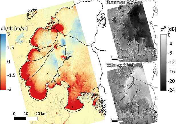
Figure 5. Surface elevation change rate (m yr−1) over Vatnajökull Ice Cap (Iceland) from TanDEM-X bistatic acquisitions in summer 2012 and winter 2016. The right panels show the backscatter images (dB) for these two periods, illustrating the strong seasonal contrast and the need for correcting the varying radar penetration into snow and firn. A larger penetration depth is expected in the cold winter snow and firn (high backscatter) compared to the wet summer firn (low backscatter).
Download figure:
Standard image High-resolution imageFor large basins and on the flat areas at the interior of the ice sheets, TanDEM-X elevation change maps can be complemented with interpolated CryoSat-2 elevation changes at crossover locations (Krieger et al 2020).
3.3.2. Limitations and challenges of InSAR DEMs for elevation change mapping.
3.3.2.1. DEM processing and phase unwrapping errors.
The ruggedness of the topography of many glacierised regions with steep mountains and intricate water bodies poses a significant difficulty for the interferometric processor algorithms of phase unwrapping and absolute elevation determination (Rossi et al 2012). Most of these issues can be overcome by exploiting a robust external reference DEM like the global TanDEM-X DEM in case of multitemporal TanDEM-X DEM generation.
3.3.2.2. DEM coregistration.
The reference and secondary DEMs may be affected by vertical biases with respect to each other. These can be constant (offset), linear (tilt) or even varying with low frequency (e.g. Malz et al 2018, Abdel Jaber et al 2019). They can furthermore be affected by horizontal shifts causing an additional slope- and aspect-dependent elevation bias in the surface elevation change, which couples with the vertical bias, resulting in a systematic error with high potential impact on the volume change rate estimated over large areas.
3.3.2.3. Signal penetration.
For the analysis and interpretation of interferometric elevation over snow and ice, the effects of signal penetration have to be considered (Dehecq et al 2016, Lambrecht et al 2018, Rott et al 2021, Sommer et al 2022). These effects become more prominent with increasing radar wavelength so that comparison of DEMs derived from SAR sensors operating at different wavelengths can be challenging. The elevation difference bias can also be large if SAR DEMs are compared to DEMs derived from optical images as the former are subject to radar penetration whereas the latter map the glacier surface (Li et al 2021). The surface inferred from InSAR elevation data refers to the position of the scattering phase centre in the snow/firn medium, which may result in an elevation bias versus the actual surface (Dall 2007). Ideally, the InSAR data over temperate glaciers should be acquired in warm seasons in order to reduce the SAR signal penetration. The status of the snow and firn surface of a glacier in respect to wetness and possible effects of radar signal penetration can be assessed through the analysis of backscattering coefficients measured by the active SAR and included in the systematic error budget (Abdel Jaber et al 2019). However, on the rough crevassed termini of temperate glaciers, the surface scattering is dominating and the SAR signal penetration is minimal.
3.3.2.4. Imaging geometry.
In complex topography areas, information in SAR images is lost due to radar layover and shadow effects. This can be partially compensated by combining data acquired from ascending and descending orbits. In the case of InSAR DEMs because the incidence angle on the glacier surface varies in range direction, it cannot be identical in the opposite viewing geometries and leads to differences in SAR signal penetration. Besides, few areas are always either in layover or shadow and can never be resolved in the SAR image.
3.3.2.5. Seasonal changes.
Ideally, data acquisitions should be at the end of the ablation season (also the end of the glaciological year) when the glacier surface is at its lowest, but most importantly the two coverages should be acquired at the same time of year in order to minimise seasonal changes, which can be significant in certain glacier regions (Sommer et al 2022). Since in general data availability restricts the ability to fulfil this criterion, the residual temporal gap has to be compensated for, and taken into account in the systematic error budget.
3.3.3. Future missions with single pass InSAR capabilities.
The German Space Agency (DLR) plans to release TanDEM-X DEM 2020 in 2024, a new global DEM which will combine bistatic TanDEM-X data acquisitions between 2017 and 2020. Beforehand a 30 m change map indicating regions with significant height changes to the TanDEM-X DEM (released in 2018) will be made available in 2023.
The High Resolution Wide Swath (HRWS) DLR mission aims at continuing the X-band series and is programmed to be launched in 2026/2027 (Moreira et al 2021). HRWS consists of a main high-resolution X-band radar satellite and three small, receive-only satellites in formation flight. The small satellites, following the MirrorSAR concept (Krieger et al 2018), have a reduced functionality compared to classical receiver satellites and allow an effective, low-cost implementation of a multistatic interferometric system for high-resolution DEM generation and for secondary mission objectives such as ocean currents, traffic flow monitoring, river and ice flow monitoring using along-track interferometry. The multistatic mission goal will be a global DEM at 4 m posting with a relative elevation accuracy of 2 m. The flexibility of HRWS's multistatic mission design will allow the generation of on-demand local to regional DEMs.
Harmony, selected as European space agency (ESA)'s Earth Explorer 10 will be launched in 2029 to address key scientific questions related to ocean, ice and land dynamics. It is envisaged as a mission with two receive-only C-Band synthetic aperture radar (SAR) satellites that orbit in two alternative formations with the Copernicus Sentinel-1D satellite as transmitter. In the cross-track interferometry constellation planned for years one and five of the mission, and perhaps intermediate periods, Harmony will produce interferometric DEMs over virtually all glaciers globally and with the same repeat as Sentinel-1D, i.e. nominally 12 d.
Two European companies, ICEYE and SATLANTIS, announced recently preliminary plans to develop and manufacture a Tandem for Earth Observation (Tandem4EO) constellation consisting of two radar and two very high resolution (VHR) optical satellites, each capable of under 1 m resolution imaging. The satellites are to be flown in a sun-synchronous orbit, with two ICEYE SAR imaging spacecraft flying in a bistatic formation, and two SATLANTIS very high-resolution optical imaging spacecraft trailing behind. With closely coordinated operations, the constellation intends to support, among other themes, environmental monitoring at land and sea as well as precise SAR Interferometry (InSAR) change detection, thus being also of interest for glacier studies.
4. Radar altimetry
Earth observing radar altimetry has traditionally been used to derive time-dependent elevation over oceans and ice sheets. The large (∼10 km) footprint of conventional radar altimetry has limited its application over regions of more complex topography. The launch of CryoSat-2 20 (Wingham et al 2006) by the European Space Agency in 2010 changed this however, allowing the monitoring of glaciers outside the two large ice sheets (McMillan et al 2014, Gray et al 2015, Foresta et al 2016, Jakob et al 2021).
4.1. Radar altimetry data
Radar altimetry for Earth observation was initially developed for observing ocean topography and is one of the main instrumental records of ocean topography with applications in marine geoid, ocean currents, and sea level change. Its use is now ubiquitous across the cryosphere and inland water. Radar altimeters are nadir-looking instruments recording time between pulse emission and reception, which is then converted to distance. This distance is usually that of the point-of-closest approach (POCA), obtained via retracking of the recorded waveform (Martin et al 1983, Wingham et al 1986, Davis and Moore 1993). Over sloping terrain, POCA is situated off-nadir and requires special procedures to properly relocate the echo (Brenner et al 1983). CryoSat-2 operates a beam-forming radar altimeter which improves the along-track footprint resolution, and its interferometric mode allows accurate echo-location in the across-track direction (figure 6).
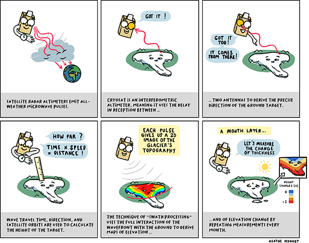
Figure 6. Principles of CryoSat-2 interferometric radar altimetry and swath processing. Image credit: Agathe Monnot.
Download figure:
Standard image High-resolution imageThis revolutionary design led to a paradigm shift in how radar signal is processed for elevation retrieval. In the presence of sloping terrain, CryoSat-2 is akin to the geometry of a side-looking SAR, with the ability to retrieve elevation information beyond the POCA (Wingham et al 2006). The potential of the so-called swath processing has been demonstrated with data acquired by the airborne ASIRAS radar system (Hawley et al 2009) and then by CryoSat-2 (Gray et al 2013, Gourmelen et al 2018), generating between 1 and 2 orders more measurements than POCA from conventional waveform retracking. For a detailed description of swath processing, we refer to Gray et al (2013) and Gourmelen et al (2018). Apart from an increase in the number of elevation measurements retrieved from CryoSat-2, swath processing allows a better sampling of low-lying terrain as the POCA tends to be located in topographic highs (Foresta et al 2016). This leads to a more complete hypsometric coverage of small ice bodies and thus a more representative sampling of ice elevation changes that tends to be strongly correlated with elevation. In addition, since it does not rely on waveform retracking, swath processing allows retrieval of elevation even when the waveform leading edge is difficult to identify such as for high surface slopes and high terrain roughness. The improved spatial coverage coupled with a monthly repeat cycle gives CryoSat-2 unique spatio-temporal capabilities to monitor changes in glacier volume, and ultimately mass.
4.2. Principle to assess glacier changes
To assess linear rates of change from swath elevations, the method follows a generic approach developed over ice sheets. The swath elevation data is binned into a grid, with cell resolution typically set around 500 m as a trade-off between spatial resolution and robustness, and then a plane-fit approach is applied in each grid cell (Foresta et al 2016, 2018). The plane-fit algorithm is a simple regression, modelling elevation (z) with the parameters easting (x), northing (y) and time (t). The coefficient for time (t) resolves a constant rate of surface elevation change and is retrieved from the plane-fit model of each individual grid cell, resulting in gridded maps of dh/dt. Several improvements to the method have been made by applying outlier removal, quality filtering and quality weighting methods (Foresta et al 2016, 2018, Morris et al 2020, Jakob et al 2021, Morris et al 2022). The maps of elevation changes typically have coverage of between 60% and 87% (Foresta et al 2016, 2018, Morris et al 2020, Tepes et al 2021). Different gap filling methods have been applied over the years, including spatial interpolation and hypsometric averaging at different spatial scales (Nilsson et al 2015b). Similar to the DEM differencing and laser altimetry methods, the elevation changes are then converted into mass changes, using the glacierised area from glacier masks (section 2) and a volume-to-mass conversion factor (section 3.1).
In regions with highly complex terrain, such as High Mountain Asia and the Gulf of Alaska, the data rate is usually lower due to limitations with closed-loop onboard-tracking (Dehecq et al 2013) and decreasing data quality with higher surface slopes. Larger grid cells are therefore necessary, and since for larger grid cells the plane-fit approach is a too simplistic representation of topography, an auxiliary baseline DEM is required to remove the terrain-related elevation change within each cell (Kääb et al 2012, Jakob et al 2021).
Besides providing linear change over a time-period, CryoSat-2's monthly repeat cycle has enabled multiple studies to resolve time-dependent changes, giving insights into annual and seasonal changes (Gray et al 2015, Foresta et al 2016, 2018, Morris et al 2020, The IMBIE Team 2020, Jakob et al 2021). For monthly change in elevation, additional spatial averaging is needed and resolution is typically set from 2 km for relatively regular surfaces (The IMBIE Team 2020) up to larger glacier units (Jakob et al 2021). Several methods for time series generation exist, from simple monthly averaging (Foresta et al 2018) to more robust statistical weighted mean (Davis and Segura 2001, Gray et al 2015, Malczyk et al 2020).
4.3. Limitations and challenges
Limitations related to other elevation change methods (DEM differencing, laser altimetry) are also applicable to radar altimetry-based studies. These include the uncertain volume-to-mass conversion, the need for gap-filling or data interpolation, and reliance on correct glacier masks for generating volume change and mass balance.
Further, Ku-band radar signal scatters within the snow and firn volume, with the potential to impact the accuracy of time-dependent elevation, with spectacular examples over the interior of the Greenland Ice Sheet after extreme melt events (Nilsson et al 2015a). This spectacular case study however stems from the combination of a thick and dry firn, and of the absence of repeated and frequent melt events. Studies conducted over a large range of settings have demonstrated the consistency between radar-altimetry and airborne laser or field-based multi-annual elevation change (Gray et al 2015, Foresta et al 2016, Gourmelen et al 2018, Tepes et al 2021), as well as ways to identify change in penetration and to correct for its impact (Nilsson et al 2015a, Slater et al 2019, Gray 2021). Scattering properties can also induce elevation biases at a seasonal timescale (Gray et al 2019, Morris et al 2022), and efforts are underway to understand and address their impact and exploit the potential of radar altimetry for mapping seasonal change.
4.4. Outlook
Over the course of the last decade, CryoSat-2 has demonstrated that beam-forming, interferometric, radar altimetry can monitor glacier change globally, providing a unique blend of spatial and temporal resolution. It offers the possibility to analyse glacier change in response to complex atmospheric and oceanic forcing. The combination of radar altimetry with other available techniques and constantly improving glacier and climate models should lead to more accurate mass balance estimates and better process understanding.
Importantly, the European Commission Copernicus expansion mission concept CRISTAL (Kern et al 2020), a radar altimeter inspired by CryoSat-2 and AltiKa, and due to launch in 2027, will be the first operational mission with a primary objective to monitor glaciers globally for decades to come (figure 2).
5. Laser altimetry
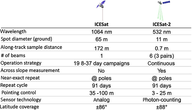
Spaceborne laser altimeters can measure the elevation of the Earth's surface at very high accuracy over a small spatial footprint. They emit a short laser pulse at a known time that reflects off of the Earth surface and back to the instrument telescope, where its arrival time is recorded and the total travel time is computed. Knowing the speed at which the laser pulse travels, the travel flight can be converted to range. With additional knowledge of the spacecraft position and orientation, range measurements can be converted to elevation measurements geolocated to a point on the Earth surface. Laser sensors record profiles of individual elevation measurements rather than spatially continuous DEMs such as from imaging sensors. There have been three Earth-orbiting satellite laser altimeter missions (table 1): NASA's Ice, Cloud and land Elevation Satellite (ICESat, 2003–2009), ICESat-2 (2018-), and GEDI (2018-). The latter is the laser altimeter on board the International Space Station (Dubayah et al 2020). It has not been extensively used so far in glaciology and is not described further here.
Table 1. Main characteristics of the ICESat and ICESat-2 missions.
|
5.1. Laser altimetry data from ICESat and ICESat-2
The main goal of ICESat was to measure the elevation change of the ice sheets to determine their contribution to sea level change (Schutz et al 2005). Despite design limitations that shortened the operational lifetime of the lasers (Abshire et al 2005), the mission provided global surface elevation measurements of unprecedented accuracy during its seven year mission life (2003–2009). ICESat recorded data during two to three month-long campaigns per year. The data consists of full-waveform 1064 nm laser returns of an ∼65 m elliptical laser footprint (Schutz et al 2005). The mission operated in a 91 day repeat orbit and a 94° inclination that covered latitudes up to ±86°, with precision pointing employed in polar regions to steer the laser footprints to within ±300 m of reference ground tracks. In lower latitudes, the reference ground track pattern was not repeated with as good accuracy. The along-track distance between measurements is 172 m, but the distance between reference ground tracks ranges from ∼6 km close to the poles up to 89 km at the equator. For land ice studies, there exist preprocessed level-2 data products: GLAH12 (optimised for ice sheets), GLAH14 (commonly used for mountain glaciers), and GLAH06 (level 1B, used for smooth polar glaciers). In addition to an elevation value for each footprint, these products include numerous attributes and corrections. The latest release of the data, 2014, is version 34. ICESat's revolutionary data provided multiple glaciological insights, in particular for volume changes of ice sheets (Pritchard et al 2009, Sørensen et al 2011) and glaciers (Gardner et al 2011, Kääb et al 2012). The success of ICESat led to the follow-up mission ICESat-2, launched eight years after the end of the ICESat mission. To bridge the gap between the two missions, NASA'S Operation IceBridge provided annual airborne altimetry data for selected areas in the Arctic and Antarctic (MacGregor et al 2021).
ICESat-2 was launched in September 2018, and had a minimum mission lifetime of three years (Markus et al 2017) met in December 2021. Unlike its predecessor, ICESat-2 uses a digital photon counting detector and 10 kHz micro-pulse laser, providing a greatly increased number of elevation measurements with 0.7 m along-track spacing between pulses (Neumann et al 2019). ICESat-2 operates in a 91 day repeat orbit, like ICESat, but with a latitude coverage up to ±88°. The laser micro-pulse is split into three-beam pairs (six beams total), with each pair consisting of a weak (¼ strength) and strong beam (full strength). Within each pair, beams are separated on the ground by 90 m and the beam pairs by 3.3 km (Markus et al 2017). The surface footprint of each beam is approximately 11 m in diameter (Luthcke et al 2021, Magruder et al 2021). Data is collected nearly continuously globally but the satellite only operates in exact repeat mode in polar regions, with a pointing control of 4.4 m (Luthcke et al 2021). At lower latitudes the mission off-points the instrument to prioritise vegetation coverage over repeat observations. Level 2A Geolocated Photons (ATL03) is the ICESat-2 product of primary interest for studies of detailed glacier features such as crevasses (Herzfeld et al 2021) or supraglacial lakes (Fair et al 2020). Most suitable for glacier change studies are Level 3A Land Ice Height (ATL06) and L3B Annual Land Ice Height (ATL11, corrected for surface slope), that are binned in the along-track in 40 m and 60 m segments, respectively. Level 3B gridded ice height and height change data (ATL14, ATL15) were made public in late 2021.
The 1064 nm laser on board ICESat led to little multiple scattering within snow and ice and therefore no elevation bias (Smith et al 2018). ICESat-2 uses a 532 nm laser that, under certain conditions, can experience a large degree of multiple scattering within the snow and ice. The magnitude of this elevation bias depends on snow conditions and the method of identifying the surface height from the photon cloud (Smith et al 2018). It can be as large as 24 cm in extreme cases (e.g. pure snow/ice with extremely large grains). However, for most applications, the bias is negligible (2–5 cm) and largely cancels for repeat measurements under similar snow conditions.
5.2. Principles to assess glacier changes
ICESat was only capable of pointing to the same location on the ground (i.e. reference ground track) to within 10s to 100s of metres and measurements were made every ca. 170 m along-track. This makes it challenging to directly compare near-repeat elevation measurements, as elevation changes will be convolved with differences in elevation due to changes in measurement location (figure 7). This is often referred to as the 'slope error' and must be corrected for. ICESat-2 has far superior pointing control (3–25 m) and closely spaced beam pairs (90 m) that make correcting for 'slope error' robust and straightforward. In steeper or rougher terrain or in the mid-latitudes without quasi-exact repeat tracks, different ground tracks may not be directly comparable altogether without an additional reference elevation dataset and the use of spatial statistics (figure 7). In all cases, the sampling is rather sparse at the scale of individual glaciers or ice caps, and most of the times uneven between the ablation and accumulation areas, such that a careful extrapolation to the entire ice body is required.
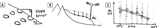
Figure 7. Calculating the regional rate of elevation changes from ICESat over steep terrain. (A) The offset of ICESat's quasi-repeat tracks causes a 'slope error': a gentle slope of α = 0.5° combined with an across-track offset of 150 m results in 1.3 m elevation difference. This has to be accounted for when assessing glacier thickening/thinning from ICESat data. (B) When altimetry ground tracks do not overlap, elevation measurements within a spatial region are compared to a common reference DEM to calculate dh. (C) The resulting dh from several years of data are plotted against time and linear regression is used to estimate glacier thinning/thickening within that glacier region. Reproduced with permission from Treichler (2017).
Download figure:
Standard image High-resolution imageWhatever the method, accurate glacier masks are required to correctly classify individual surface elevation measurements (section 2). Inclusion of measurements on stable terrain outside glaciers (e.g. when an outdated glacier inventory is used) will lead to almost unbiased volume change estimates (the off glacier elevation changes will sum up to almost 0) but an underestimate of glacier thickening/thinning area-averaged rates because the correct total volume change is divided by an area which is too large.
5.2.1. Methods for calculating elevation change from near-repeat observations.
All methods to estimate elevation change from ICESat data aim at removing the influence of sloping terrain between slightly shifted repeat ground tracks (figure 7(A)). Moholdt et al (2010) provide an overview and comparison of the most common methods summarised hereafter. The most accurate way to retrieve elevation change is to compare elevation profiles at locations where ascending and descending tracks intersect (i.e. crossover locations) (Brenner et al 2007), but crossover locations can be sparse. Another set of methods use along-track planes formed by segments of repeat ground tracks, relying on redundancy from several years of laser altimetry measurements. In this approach linear regression is used to simultaneously estimate the local surface slope and elevation change from ice thinning/thickening (Fricker and Padman 2002, Howat et al 2008). Most variants of this method assume that the surface slope and rate of elevation change are constant over several years, though higher order models can also be fitted (Nilsson et al 2016). This approach can be sensitive to how the tracks are ordered in space. Schenk and Csatho (2012) found that higher-order fitting surfaces better captured the more complicated thinning/thickening signal in the rapidly changing coastal areas of the ice sheets. A third method relies on a DEM to estimate, and correct for, the terrain differences between repeat ground tracks (Slobbe et al 2008). A variant of this last method is also applicable to non-repeat measurements and is discussed in section 5.2.2.
All of the above methods are most applicable to ICESat data and less relevant to ICESat-2 data, when ICESat-2 data is acquired along repeated reference ground tracks. ICESat-2 has exceptionally precise pointing capabilities (Luthcke et al 2021) that often negates the need for any 'slope error' correction. ICESat-2 is also equipped with closely separated beam pairs that allow for easy translation of non-exact repeat measurements to a common reference ground track. This correction is applied on the ATL11 data product.
5.2.2. Methods for non-repeat observations and rough surfaces.
Outside the polar regions, repeat tracks of ICESat/ICESat-2 are not close enough to be compared directly. Furthermore, the rougher surfaces of small glaciers cause greater uncertainties in individual elevation measurements. It is thus more practical to normalise all ICESat/ICESat-2 surface elevation measurements from several years with the help of a reference DEM surface. This method is described by Treichler (2017) and is suitable for mountain glacier studies. Thereby, individual laser altimetry measurements are compared to a reference DEM of a known date (figure 7(B)), and only the resulting elevation differences are analysed. Surface elevation change over time (dh/dt) is then estimated by fitting a linear regression to dh from different years against time (figure 7(C)). The result is a single dh/dt estimate for the analysed group of elevation samples. In the case of ICESat, given the sparse ground tracks, this is often a rather large area such as an entire mountain range. There are some caveats with this method: (a) the elevation differences to the reference DEM (dh) contain both real elevation changes between the DEM and laser altimetry data as well as uncertainties and potential bias in either the DEM, the laser altimeter data, or both; and (b) dh have to be binned spatially and filtered to remove outliers and make sure that they are representative for the glaciers in the sampled area. Careful preprocessing is vital to reach reliable results, in particular a robust assessment of biases and uncertainties in the reference DEM, elevation biases from snow cover during ICESat/ICESat-2 acquisitions, and the elevation distribution of the laser altimetry samples (Treichler et al 2019). This approach has been applied to the larger glacierised regions across the globe and in particular to High Mountain Asia, where glacier changes were poorly known before ICESat data became available (Kääb et al 2012, Gardner et al 2013, Farinotti et al 2015, Treichler et al 2019). The increased number of measurements provided by ICESat-2, relative to ICESat, significantly augment the utility and accuracy of this approach.
5.3. Outlook
New methods take time to develop for new products like ICESat-2, and as of this writing, there are relatively few results in the literature. It is expected that ICESat-2 data will contribute to new insights and a much better understanding of the entire cryosphere, including dynamical changes of the ice sheets (Smith et al 2020) and improved monitoring of mountain glaciers (Wang et al 2021, Fan et al 2022), but also advances in related disciplines such as, snow depths on- and off-glacier (Treichler and Kääb 2017), sea ice and ice shelf thickness (Kacimi and Kwok 2020) or permafrost changes (Michaelides et al 2021). In addition, the accurate elevation measurements of both ICESat and ICESat-2 provide a globally consistent reference elevation dataset that has the potential to greatly improve the quality and accuracy of existing and upcoming DEMs and other elevation data across the globe, which will directly benefit glacier volume change studies.
There are currently no funded Earth observing laser altimetry missions under development. However, the need for the continuation of cryosphere focused laser altimetry is highlighted in the 2018 Decadal Survey for Earth Science and Applications from Space, a guiding document for NASA's future Earth science investment, and has been recommended as one of seven observables to be completed as an Earth System Explorer class mission.
6. Gravimetry
The gravity recovery and climate experiment (GRACE) follow-on (FO) satellites provide a unique way to track mass redistribution on global scales. Launched in 2018, they continue the measurements of the GRACE mission, which was operational from 2002 to 2017 (Tapley et al 2004, Landerer et al 2020). Both missions consist of a pair of satellites in the same orbit but separated by about 200 km and are based on the same principle: given that the satellites are at different locations in their shared orbit, each of them will be affected differently by the Earth's gravitational field. For example, if the two satellites approach a mass anomaly on or within the Earth, such as a mountain range, the first satellite will experience its gravitational pull stronger and earlier than the other one. This results in an unequal acceleration of the satellites and changes their relative velocity, and consequently the inter-satellite distance. These extremely small changes in distance and velocity are measured by a very precise ranging system in the satellites. Global navigation satellite systems receivers simultaneously record the location of the satellites, and the orientation of the satellites in space is derived from a star-camera system. Forces not related to the gravitational field, for example atmospheric drag and solar radiation pressure, are measured by on-board accelerometers which are precisely aligned with the centre of gravity of the satellites so that they only measure non-gravitational forces.
6.1. GRACE and GRACE-FO data
The Earth's gravitational field is described by the geopotential V, i.e. the potential energy per unit mass at a certain point. At a point above the Earth's surface, with spherical coordinates radius r, co-latitude θ and longitude λ, it can be expressed as a sum of Legendre functions:
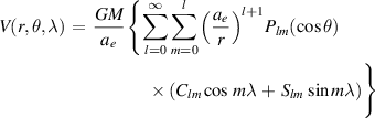
where G is the gravitational constant, M the mass of the Earth and ae denotes its mean equatorial radius. Plm are the Legendre polynomials of degree l and order m, and Clm and Slm are spherical harmonic coefficients. For further details, we refer the reader to Wahr et al (1998). As can be seen from the formula above, coefficients with a higher degree and order are related to increasingly smaller wavelengths. At the same time, the scaling by (ae /r)l +1 implies that the effect of these coefficients have a smaller contribution to the geopotential than the lower-order coefficients. In practice, this means that the orbit of the GRACE satellites are dominated by the large-scale mass distribution of the Earth and that small-scale features, such as glacier mass changes, are more challenging to measure than large-scale features, such as ice-sheet wide mass changes.
By collecting a sufficient amount of range-rate observations, a model of the Earth's gravity field can be derived. The GRACE/GRACE-FO mission provides updated gravity fields typically every month, although weekly or even daily updates are available as well (at the cost of a lower resolution).
At seasonal to decadal time scales, variations in the gravity field are mainly induced by redistribution of water on the Earth's surface, although processes within its interior such as glacial isostatic adjustment (GIA) may contribute as well, as we will see later on. Using an appropriate scaling (see Wahr et al 1998 for details), variations in the geopotential can be expressed as variations in surface water loading. This is usually expressed in units of metre water equivalent height. It should be kept in mind that GRACE can only measure anomalies in surface water loading, not the absolute weight of a glacier or ice sheet.
GRACE data are distributed by the GRACE science data centres, and other parties, as spherical harmonics (the Clm and Slm coefficients in the equation above). Since higher-order coefficients are increasingly affected by observational noise, only coefficients up to degrees and orders smaller than 60 or 90 are typically used in the derivation of the surface water loading anomalies, which corresponds to a maximum spatial resolution of approximately 200–300 km. A user-friendly alternative for the spherical harmonics are mascons, i.e. mass concentration blocks. These provide local mass variations on a regularly spaced grid. Compared to the spherical harmonics, they are less affected by noise and therefore require little or no post-processing. Mascons products are available with a grid resolution down to a few tens of kilometres, but it should be kept in mind that the inherent resolution is still in the order of a few hundred kilometres (in other words, the signal in adjacent grid cells will be correlated). Furthermore, once the grid cells are predefined by the processing centres, they do not always cover the area of interest exactly and may contain signals from neighbouring ice bodies (such as the Greenland Ice Sheet when studying the glaciers of the Canadian Archipelago or in Iceland (Sørensen et al 2017)) or other non-glacier signals (e.g. groundwater and soil moisture signals in Patagonia or High Mountain Asia).
6.2. Glacier mass balance from GRACE
Figure 8 illustrates the linear trend in surface water load as observed by GRACE/GRACE-FO from 2002 to 2021. Together with the polar ice sheets, mountain glacier regions stand out with rates in the order of 20–50 cm yr−1 water equivalent mass loss in Alaska, the Arctic Archipelagos and Iceland.

Figure 8. Trends in the global surface mass distribution between April 2002 and January 2021, expressed in centimetres equivalent water height per year, based on CSR mascons (Save et al 2016). Yellow to red colours indicate a mass loss, with extreme values in the polar regions reaching −90 cm yr−1.
Download figure:
Standard image High-resolution imageTo obtain the total mass balance for a region, the local surface mass anomalies need to be summed up over the region of interest. When working with mascons, this is relatively straightforward, but for the spherical harmonics some intermediate steps are required. If the Stokes coefficients were available up to an infinite degree l, we would be able to create a perfect region mask and could simply integrate the mass anomalies over the region. However, as mentioned earlier, the spherical harmonics are only provided up to a limited degree, typically 60 or 90. This, together with the postprocessing often applied to reduce noise in the higher degree coefficients, leads to attenuation and spreading of the signal (Swenson and Wahr 2002). Here, spreading (or leakage) means that due to the limited resolution of the gravimetry data, mass variations from adjacent areas will spill into the region of interest. Likewise, part of the signal in the region of interest will be spread out beyond the boundaries of that region, e.g. in the ocean although recent mascon approaches minimise this effect compared to former spherical harmonic solutions (Wiese et al 2016). Only considering the glacierised areas would therefore result in a biased estimate. Several methods have been proposed to circumvent these limitations. The most common approach is to place one or several unit mass loads in the glacierised areas of interest, represent these as Stokes coefficients with the same characteristics as the GRACE mass anomaly data (e.g. limited to the same maximum degree and applying a similar post processing) and finally applying a scaling to the mass loads so that the difference with the actual GRACE observations is minimised (Wouters et al 2008, 2019, Jacob et al 2012, Chen et al 2013, Gardner et al 2013, Ciracì et al 2020).
6.3. Limitations and challenges
Just like any satellite observation, the GRACE data comes with noise, which reflects itself as random fluctuations in the mass anomaly time series in the order of a few gigatons. This means that in regions where the glacier mass change signal is small, the signal-to-noise ratio will be small, and the GRACE results should be interpreted with care. For the larger glacier regions, however, GRACE can capture mass variations with a high degree of confidence.
Even after extracting the mass changes in the glacier regions, there are confounding processes that need to be removed to isolate the glacier signal. Because GRACE has no vertical resolution, it senses the integrated sum of mass redistribution within its footprint, i.e. the sum of the water load changes at the surface and those in the subsurface. Many glaciers are located in regions that were widely covered by thick layers of ice during the Last Glacial Maximum (about 20 kyr ago), which depressed the Earth's surface and led to mass redistribution in the Earth's mantle. This ice has disappeared since, but the Earth's highly-viscous mantle material is still readjusting to the changes in surface load. The associated mass redistribution in the mantle will also be observed by the GRACE satellites. Several models exist to correct for this process, called GIA, which can be used to correct the GRACE data. Whereas models show a wide spread in Antarctica (Martín-Español et al 2016), they are fairly well constrained in mountain glacier regions and the Arctic and GIA mass rates agree in most regions within a few Gt yr−1 (Blazquez et al 2018). Yet, when summed over all glacier regions globally, differences become significant. For example, the GIA corrections used in two of the most recent GRACE-based glacier mass balances studies, Ciracì et al (2020) and Wouters et al (2019) amounted to 58 ± 11 Gt yr−1 and 34 ± 21 Gt yr−1, respectively ca. 18% and 13% of the total glacier mass change signal (figure 9). Furthermore, some regions with a low mantle viscosity are still adjusting to the load changes related to the Little Ice Age (Sørensen et al 2017). A similar model-based correction is applied for this, although these models are underconstrained in some areas and not all studies include this correction. Another solid earth effect, i.e. mass redistribution associated with earthquakes, is harder to correct for, but is mostly of small magnitude and manifests itself as a step change in the mass time series followed by a slow recovery. In the few cases where this affects glacier mass balance estimates, this can often be identified visually.
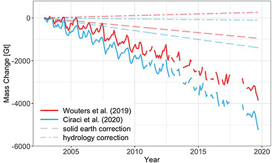
Figure 9. Global glacier mass change (Gt) time series for April 2002–September 2019 from GRACE and GRACE follow-on (Wouters et al 2019, Ciracì et al 2020). The thick lines show the cumulative mass change, the dashed lines the corrections for long-term hydrology (dashed-dot) and solid earth (long dashes) effects. The different corrections applied in the two studies explain for a large part the divergence of the glacier mass change time series.
Download figure:
Standard image High-resolution imageThe coarse resolution of the GRACE observations also implies that, even after correcting for GIA, the signal is a mix of mass changes related to glaciers and hydrological processes, such as changes in the surface, canopy and soil moisture water storage, and in the groundwater table. This is practically an issue in regions where glaciers are scattered and small compared to GRACE's footprint, for example in Central Europe and the Caucasus. Furthermore, strong hydrological variations outside the region of interest may affect the glacier mass balance estimates through the leakage effect discussed earlier (An et al 2021). Again, this is accounted for using models, where it should be noted that most models only represent part of the hydrological cycle, e.g. excluding groundwater storage changes and anthropogenic influences, and tend to underestimate long-term changes in hydrological water storage (Scanlon et al 2018). Furthermore, the magnitude of corrections depends strongly on the choice of the model. The global hydrology correction summed up to +6 ± 7 Gt yr−1 in Ciracì et al (2020) vs. −11 ± 6 Gt yr−1 in Wouters et al (2019) using a different model. Because of the disagreement between models, some studies prefer to omit the correction and include it as an uncertainty (Reager et al 2016). Whereas the impact of hydrology is small in the polar regions, it is the major source of uncertainty for most mid-latitude glacier systems. A further complication is that if part of the glacial meltwater runs off in a proglacial lake, a nearby endorheic lake or an aquifer, the net local mass change detected by the GRACE satellites will be smaller than the actual glacier mass loss. Since such processes are currently not included in hydrological models, this will lead to an underestimation of glacier mass balance. Finally, leakage of the glacier mass change signal in the ocean can also be an issue for glacier regions fringing the ocean. This effect is reduced in the mascon-based solutions.
6.4. Outlook
The GRACE-FO mission is currently our only tool to directly monitor glacier mass changes at a global scale, i.e. without a volume to mass conversion. Although it comes with its own limitations, it has proven to be essential to study the response of the larger glacier systems to climate variability. Likewise, the GRACE/GRACE-FO data has become an indispensable source of information in many other fields, and the importance of continued observations has been recognized by the wider scientific community and decision makers (Tapley et al 2019). Several initiatives, including a joint effort of NASA and ESA, have recently emerged to study concepts for future gravity missions (respectively named Mass Change and MAGIC), consisting of one or more pairs of satellites. This would lead to an improved spatial and temporal resolution of the observations, and most importantly, continuity of this unique time series of global glacier mass balance that started in 2002 with the launch of the GRACE satellites.
7. Strengths and weaknesses of the different techniques
7.1. Comparison over the Vatnajökull Ice Cap—Iceland
The different methods presented in this review are applied to the Vatnajökull Ice Cap, a ∼8000 km2 ice mass located in Southeast Iceland (figure 10). The goal of this comparison is not to single out the best-performing technique or to provide a reconcile mass change estimate, but rather to illustrate the capabilities and characteristics of all these techniques in a concrete case study.
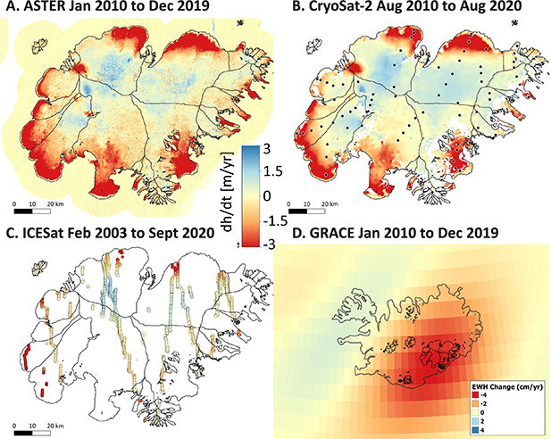
Figure 10. The elevation and mass changes estimates of the Vatnajökull Ice Cap (Iceland). The upper row shows dh/dt (A) applying Gaussian process regression to a time series of ASTER DEMs (Hugonnet et al 2021) and (B) using CryoSat-2 swath processing (Foresta et al 2016, updated). The lower panels show (C) dh/dt from ICESat and ICESat-2 (unpublished) and (D) the GRACE/GRACE-FO derived mass change anomaly for entire Iceland (Wouters et al 2019, updated). For CryoSat-2, dh/dt is obtained by fitting a linear trend to the elevation time series, whereas for other methods it is derived as the difference between the end and start elevations, divided by the time separation. The InSAR dh/dt map for Western Vatnajökull is shown in figure 5 with the same colour scale as panels (A)–(C). The black dots in panel B locate in situ surface mass balance measurements performed by the University of Iceland (Aðalgeirsdóttir et al 2020).
Download figure:
Standard image High-resolution imageVatnajökull is large enough so that each technique can (almost) resolve it spatially. Another advantage is that comprehensive glaciological field surveys are available (Björnsson et al 2013, Aðalgeirsdóttir et al 2020). These in situ data measure the SMB and have been performed seasonally since September 1991. In Aðalgeirsdóttir et al (2020), the SMB was corrected for non-SMB components and calving fluxes (Jóhannesson et al 2020) to calculate the total mass balance, the quantity directly comparable to the remote sensing estimates. Applying or not this challenging correction leads to strikingly different results, this is the reason why both time series (i.e. with/without non SMB components) are retained in figure 11.
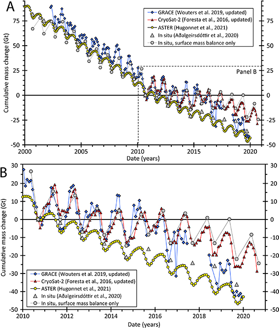
Figure 11. Time series of cumulative mass change (Gt) for Vatnajökull from the different techniques during 2000–2020 (upper panel). The lower panel zooms in over 2010–2020, the period common to most techniques. Cumulative mass changes are shown as anomalies compared to 15 September 2010. ICESat estimates are not included because the elevation difference measurements shown in figure 10(C) cover a varying time stamp. The main text explains why two time series derived from in situ measurements are included (see beginning of section 7.1).
Download figure:
Standard image High-resolution imageThe dh/dt map derived from InSAR TanDEM-X DEMs for West Vatnajökull was shown in an earlier section of this review (figure 5). In principle, a complete coverage of the ice cap could be derived from InSAR DEMs at high spatial resolution. Despite a shorter survey period (3.5 years), the spatial pattern of elevation changes for West Vatnajökull is highly similar to the pattern obtained from stereo-imagery and CryoSat-2 swath altimetry. The spatial resolution of the InSAR dh/dt map (6 m) is an order of magnitude higher than the one from ASTER (100 m) and almost two orders of magnitude higher than for CryoSat-2 (500 m). Fine details of the elevation changes are captured in the InSAR map (e.g. the drainage of the Skaftá cauldrons, Magnússon et al 2021). If a complete map of elevation change was available from TanDEM-X DEMs, the specific challenges to derive an unbiased estimate of the mass balance would be the need (a) to account for temporal changes in X-band radar penetration and (b) to correct the seasonal bias due to the varying acquisition dates of the DEMs.
The dh/dt map based on ASTER DEMs (figure 10(A)) has a 100 m posting to reduce computing time in a recent global scale study (Hugonnet et al 2021) but could potentially be derived at 30 m which is the posting of ASTER DEMs. The map is gap-free thanks to the relatively good abundance of ASTER DEMs over Iceland compared to other regions on Earth. The massive thinning toward glacier fronts and the surface expression of subglacial volcanic activities (such as the Bárðarbunga caldera collapse (Gudmundsson et al 2016)) are well captured. A larger noise level is observed in the accumulation areas (where the thickening is less homogeneous, noisier than for CryoSat-2), a consequence of the limited radiometric dynamic in the eight-bit ASTER stereo-imagery over homogeneous snowfields (figure 4). The time series of cumulative mass change (figure 11) exhibits a mean seasonal cycle of lower amplitude compared to other techniques and only resolves the variability over periods longer than 4–5 years. One should note that this continuous time series, obtained through Gaussian Process regression, is predicted at a monthly time step but is derived from the temporal interpolation of moderate precision and temporally inconsistent ASTER acquisitions (50 in 20 years, on average). Hence, the inter-annual variability of the mass change, e.g. the positive mass balance during glaciological year 2014–2015 or the strongly negative mass balance in 2009–2010 following the Eyjafjallajökull volcanic eruption (Aðalgeirsdóttir et al 2020), is not captured.
CryoSat-2 swath altimetry also provides an almost complete dh/dt map, covering 85% of the ice cap area (figure 10(B)). To calculate an ice cap-wide mass balance, gaps are filled using the regional hypsometric approach (McNabb et al 2019), i.e. using the mean elevation changes of the rest of the ice cap at the same altitude band. CryoSat-2 captures subtle changes in the ice cap interior as well as rapid changes related to the Bárðarbunga caldera collapse or strong thinning at the margins. There is some data loss over the steeper, marginal, parts of the ice cap, including the rapidly thinning margins. CryoSat-2 provides a smooth and continuous time series with monthly estimates thanks to the satellite's repeat period. The monthly repeat allows resolving the seasonal and inter-annual changes, with an amplitude in good agreement with GRACE (before 2016) and with the SMB measurements uncorrected for non surface-mass-balance processes.
Laser altimetry does not allow continuous temporal sampling due to the gap between ICESat (ending in 2009) and ICESat-2 (launched in 2018). Figure 10(C) shows elevation change rates from ICESat (GLAH06 L1B Global Elevation Data v34: Zwally et al 2014) and ICESat-2 (ATL06 L3A Land Ice Height, Version 3: Smith et al 2021) data. The data span the period February 2003 to September 2020. Rates of change are determined by solving least squares fits of offset, rate and seasonality to elevation anomalies within a 480 m radius of solution points that are separated by 480 m which explain the 'stepwise' lines of measurements (figure 10(C)). Elevation anomalies are determined relative to the ArcticDEM 8-m Mosaicked DEM v3 (Porter et al 2018). Despite a rather scarce spatial sampling, laser altimetry is able to capture the main patterns of change, with thinning in the lower reaches and slight thickening in the accumulation area of the two largest outlets of northern Vatnajökull (Dyngjujökull and Brúarjökull). However, ICESat/ICESat-2 has no measurement below 450 m a.s.l. and misses the very strong thinning rate on the tongues of the south and south-east flowing outlets. Given this sparse spatial sampling of a complex pattern of elevation changes, we did not attempt here to estimate the total volume and mass change of Vatnajökull. Hence, laser altimetry data are not plotted in figure 11 and not listed in table 2.
Table 2. Summary of pluri-annual rates of mass changes (Gt yr−1) of the Vatnajökull Ice Cap from different techniques. The non surface mass balance components amount to roughly −1.5 Gt yr−1. Uncertainties are provided at the 95% confidence interval.
| DEM differencing (Hugonnet et al 2021) | Gravimetry (Wouters et al 2019, updated) | CryoSat-2 altimetry (Foresta et al 2016 updated) | Glaciological, accounting for non-surface mass balance processes (Aðalgeirsdóttir et al 2020) | |
|---|---|---|---|---|
| September 2002 to September 2019 | −6.5 ± 1.0 | −7.0 ± 1.2 | NaN | −6.3 ± 1.6 |
| September 2010 to September 2019 | −5.1 ± 1.0 | −4.4 ± 1.3 | −2.9 ± 1.1 | −4.0 ± 1.6 |
Due to their coarse spatial resolution, gravimetric observations are not able to resolve Vatnajökull mass change alone (figure 10(D)). We corrected the GRACE-based mass change for entire Iceland (updated from Wouters et al 2019), with a scaling factor (0.68) deduced from an analysis of glacier mass change for all major ice masses in Iceland, as 68% of the glacier mass loss in Iceland from 2000/2001 to 2018/2019 originates from Vatnajökull (Aðalgeirsdóttir et al 2020). The processing of GRACE data was detailed in section 6. In Iceland, particular attention needs to be paid to leakage from the Greenland Ice Sheet or to the ocean together with solid Earth processes, related to mass load changes from GIA and little ice age (Sørensen et al 2011). The seasonal cycle is not as smooth as the one from CryoSat-2 with spikes in the time series, due to measurement noise and the leakage from seasonal snow in the surroundings of the ice cap. The GRACE time series also seems to diverge from the SMB-only in situ and CryoSat-2 measurements after 2016, when it gets close to the ASTER-based results and the glaciological measurements corrected for mass losses not occurring at the surface. Reasons for these differences in the time series remain unclear. This may be explained by less reliable measurements towards the end of the GRACE mission and the fact that GRACE/GRACE_FO also captures the mass loss by other Icelandic ice caps. However, a recent study found a good agreement between GRACE and CryoSat-2 mass balance time series for all icelandic ice caps lumped together (Noël et al 2022). Hence, a careful comparison of the CryoSat-2 time series from different research groups is needed.
GRACE excluded, all satellite-based techniques include a conversion of the volume change to mass change, which is done here using an average value of 850 kg m−3 (Huss 2013). This value is in principle valid for periods of more than five years (ideally more) and more appropriate for negative mass balance years. This uncertain volume-to-mass conversion remains a major challenge and partly jeopardises the usage of geodetic observations at high temporal resolution. It can easily explain some of the observed differences with GRACE and the in situ measurements, especially during years of balanced or positive mass budgets. Volcanic activity is another source of discrepancies: a striking example is the 65 m collapse (∼2 km3) of the Bárðarbunga caldera in 2014 in the northwest of Vatnajökull (Gudmundsson et al 2016) that can be wrongly attributed to glacier change by elevation change methods.
The average rates of mass change for two different periods are compared in table 2. Over the longest common period (15 September 2002–15 September 2019), the three available estimates show a satisfactory agreement, within ∼10%. However, over the shorter nine year period (15 September 2010–15 September 2019), differences get larger (±25%) with reduced mass loss from CryoSat-2, higher mass loss from ASTER DEMs and intermediate values for GRACE and the 'in situ' measurements corrected for the non-surface components (geothermal melting, volcanic eruptions, the energy dissipation in the flow of water and ice, and calving). Without this correction, in situ measurements are in agreement with CryoSat-2. It is beyond the scope of this review to conclude on the origin of these differences. Understanding them and providing a reconciled estimate of mass change require further work, in particular by examining individual glaciers of the ice cap.
7.2. Comparison over the Everest area—Himalaya
To complement the above case study over a large and flat arctic ice cap (Vatnajökull), we illustrate in figure 12 the ability of the different elevation change methods to sample spatially and temporally glaciers in mountainous areas. The study area covers 100 km by 100 km around Mt Everest (Himalaya), which corresponds roughly to 1/10 of the GRACE resolution. This is why gravimetry data are not shown in this example, they simply cannot resolve glacier mass change at this scale.

Figure 12. Spatiotemporal coverage and density of the different methods near Mount Everest. (A), (B) Spatial coverage and elevation change derived from (A) KH-9 hexagon (Dehecq et al 2020) and SPOT-5 DEMs (Gardelle et al 2013), and (B) multiple ASTER DEMs processed using Gaussian Process regression (Hugonnet et al 2021). Note that the DEMs have a single timestamp and, for ASTER time series, that the temporal resolution is generally >5 years (statistically significant elevation change rate at the 95% confidence level). (C)–(E) Spatial coverage and density from altimetry over the same area with (C) ICESat footprints, (D) ICESat-2 photons and (E) CryoSat-2 strips, rendered on top of a hillshade. A single CryoSat-2 strip includes, on average, 50,000 points points for the geographic extent considered here. ICESat and ICESat-2 footprints are buffered by 200 m for visualisation purposes. CryoSat-2 swath width is fixed to an average of 1 km. Glacier outlines are shown in black. (F) Temporal coverage and temporal density of altimetry measurements. Results of the gravimetry method are not shown due to its inability to resolve changes at this resolution.
Download figure:
Standard image High-resolution imageDEM differencing resolves the changes of individual glaciers and provides an almost 50 year long record albeit with a 5–10 year resolution. There are large data gaps in the elevation change maps due to the lack of contrast, mostly in the upper accumulation areas. This is particularly the case when only two DEMs are compared (figure 12(A)). These gaps are reduced when processing a time series of ASTER DEMs (figure 12(B)). Gaps would almost vanish if DEMs were derived from 11 or 12-bits modern stereo sensors as illustrated by the complete map of elevation differences for Mera Glacier (30 km south of Mt Everest) obtained by comparing Pléiades DEMs from 2012 and 2018 (Wagnon et al 2021).
Altimetry data, from ICESat and CryoSat-2, are not able to resolve individual glaciers. They are only able to provide a region-wide mass balance estimate when aggregated over sufficiently large regions so that glaciers (in particular the different elevations bands) are well sampled. The denser sampling by CryoSat-2 swath altimetry and ICESat-2 allows resolving regions of 100 by 100 km and infer the seasonal elevation changes (Jakob et al 2021, Wang et al 2021). For ICESat, the spatial sampling was sparser and temporally more irregular so that mass loss estimates were mostly restricted to a single value (for the period 2003–2008) over large regions (Kääb et al 2015).
7.3. Synthesis of the pros and cons of each method
Table 3 summarises the characteristics, strengths and weaknesses of the remote sensing methods to measure glacier mass changes. It includes some general and well-known limitations such as the dependence on cloud-free conditions for optical stereo-images and laser altimetry and, on the other hand, the need to account for time-variable radar penetration in snow and firn for SAR interferometry or radar altimetry.
Table 3. Capabilities of the different spaceborne techniques to estimate glacier mass change. The regional scale refers to entire RGI regions. The local scale refers to, typically an area of 50–100 km2 (i.e. a large glacier or a group of glaciers).
| Technique | DEM differencing | Altimetry | Gravimetry | ||
|---|---|---|---|---|---|
| Sensor | Optical stereo-images | SAR images | Laser (ICESat, ICESat-2) | Radar (CryoSat-2) | GRACE and GRACE-FO |
| Spatial resolution/posting | Individual glaciers resolved; Down to a few metres with modern sensors | Track spacing at 60°: ∼35 km for ICESat, 8/3.3/3.3 km (between three beam pairs) for ICESat-2 | A few 100s m in moderate topography up to several km in extreme topography | ∼300 km | |
| Time span | Since 1960s | Since 2000 | 2003–2009 (ICESat) 2018- (ICESat-2) | Since 2010 | 2002–2017 (GRACE) 2018- (GRACE_FO) |
| Temporal resolution | Typically multi-year at regional scale; Down to seasonal resolution when high resolution DEMs are frequently available | Seasonal at regional scale | Monthly at large glacier/regional scale | Monthly at regional scale | |
| Coverage | Global with ASTER; Local with other sensors | Potentially global with TanDEM-X; Within 60° N–56° S for SRTM | Global | Global | Global |
| Strengths | Associated imagery for interpretation; Numerous sensors can be combined | All weather; Associated amplitude and backscatter images for interpretation | Very accurate individual measurements | All weather; continuous, homogeneous time series | Direct measurements of mass changes (no density assumption needed) |
| Weaknesses | Most sensors are commercial, except ASTER not replaced after 2023; For eight-bit sensors only: noise in the accumulation areas; clouds | Time variable penetration of the radar signal | Weather dependant; no exact repeat; Sparse or uneven sampling of ablation/accumulation areas often hampering glacier-wide estimates | Time variable penetration of the radar signal | Need to deconvolve other influencing factors (solid earth, hydrological signal): Need models to bridge the gap between GRACE and GRACE-FO |
| Uncertain volume to mass conversion | |||||
| Sub-aqueous ice losses not observed | |||||
As illustrated by our case studies in Iceland and Himalaya, the ability of these methods to resolve mass change depends on the glacier-type, their surrounding topography and the size and latitude of the area. Due to their high resolution (here decametric), DEM-based methods excel in mountainous regions hosting, mostly at low to middle latitudes, a myriad of glaciers of varying size, but generally less than 1000 km2. Mass balance can be estimated for each individual glacier, albeit with larger uncertainties for smaller ice bodies. In these regions, the generous availability of stable terrain also facilitates the DEMs coregistration and bias correction. Conversely, the rough topography and modest mean glacier size result in a sparse sampling by laser or radar altimetry so that mass balance can be only computed over large regions, typically accounting 103–104 km2 of glaciers. The gravimetric method will also be restricted to region-wide average, and the main challenge is to account for other natural and anthropogenic processes (hydrology, solid earth) influencing its mass change signal.
Over large icefields (Alaska, Patagonia) or Arctic ice caps, DEM differencing is more challenging to apply because of the scarcity of stable terrain, the need to mosaic multiple DEMs of different dates for a full coverage and, specifically for DEMs derived from pre-2010 optical images, the reduced contrasted in the flat accumulation areas. Laser and radar altimetry are well-suited providing a high temporal resolution, down to seasonal time scale. For laser altimetry this is particularly the case for polar areas where ground tracks are repeated exactly. GRACE also works well in principle, although here again the main challenge is to account properly for all non-glacier signals, generally through modelling.
A common limitation of all techniques is that none of them is able to 'see' the loss (or gain) of ice below the waterline (sub-aqueous loss or gain) for water-terminating glaciers experiencing calving front migration. This omission does not matter (or very little) for estimating the sea-level contribution as the solid freshwater of the glacier tongue is displacing salted sea water (Seehaus et al 2015).
All these limitations and sources of uncertainties lead to a relatively large spread between the mass change estimates of the different techniques. This is well illustrated by a compilation for all glaciers and ice caps in the Russian Arctic updated from Tepes et al (2021) (figure 13, table 4). For this large RGI region (covered by 51 500 km2 of glaciers), even using the same technique (Gravimetry or DEM differencing), the losses for similar time periods differ by a factor of almost two (table 4). Hence, a first step in an intercomparison exercise will consist in understanding the reasons behind the differences between similar techniques.

Figure 13. Mass change rates (Gt yr−1) for glaciers and ice caps in the Russian Arctic (total glacier area = 51 500 km2) since 2000. Estimates from remote sensing are shown with solid lines as opposed to the dashed lines for the other studies (Box et al 2018, Zemp et al 2019). The data/method used for each estimate is provided in the legend: Alti = Altimetry, Gl = Glaciological, i.e. in situ data. Uncertainties are given at the two-sigma confidence interval.
Download figure:
Standard image High-resolution image
Table 4. Rates of mass changes (Gt yr−1) in the Russian Arctic from DEM differencing and using the gravimetric method for two periods. The table illustrates how similar methods may lead to contending estimates for the same region and similar periods.
| Gravimetry | DEM differencing | |||
|---|---|---|---|---|
| Wouters et al (2019) | Ciraci et al (2020) | Stereo-images Hugonnet et al (2021) | InSAR Sommer et al (2022) | |
| January 2003 to December 2019 | −13.9 ± 1.3 | −20.3 ± 6.5 | −10.9 ± 0.9 | |
| January 2011 to December 2017 | −18.9 ± 2.5 | −25.4 ± 7.4 | −12.0 ± 2.9 | −22.2 ± 6.4 |
8. Conclusion
In this review, we presented the different techniques able to measure glacier mass change from space: DEM differencing either from stereo-imagery or from SAR interferometry, laser and radar altimetry and space gravimetry. We illustrated how they perform to survey the mass change of a large Arctic ice body, the Vatnajökull Ice Cap (Iceland) and the smaller and steeper glaciers in the Everest region (Himalaya), and discussed their strengths and weaknesses. We highlighted some differences between the different mass change estimates, especially at short time scales (seasonal or annual). For most main glacier regions, a spread exists between the different techniques, even sometimes when the same technique is applied by different research groups. At global scale, this leads to mass loss estimates varying by 20%–30% (see figure 3(B) in Hugonnet et al (2021)).
Ten years ago, a handful of field or geodetic measurements on a limited number of glaciers were available and were extrapolated to the entire world. We have now entered a new era where multiple regional, or even global, comprehensive estimates, yet not always in agreement, are available. Understanding the reasons behind these discrepancies will require careful intercomparison work. The range of size (spanning seven orders of magnitude) and numbers (>200 000) of glaciers is an additional complexity compared to ice sheets and implies that we can hardly rely on a single method that would outperform the others. Instead, a combination of sensors and methods is probably necessary to derive the best possible estimates and to cover multiple time scales. Community efforts aiming at tackling these issues, such as RAGMAC 21 are eagerly needed.
A continuity of the underlying satellite missions, with an open data policy, is of the utmost importance to maintain and improve the monitoring of the glaciers of the future, and should be a top priority on the agenda of space agencies 22 . Free and easy scientific access to all satellite data should be the rule for these future satellite missions (Pope et al 2014). Among the different techniques to measure glacier mass balance from space, continuity seems to be on-track with forthcoming satellite missions such as Harmony for SAR interferometry and CRISTAL for interferometric radar altimetry. Less clear is the continuity of the gravimetric measurements after GRACE-FO, although China has recently launched its own experimental Tianqin-1 gravity mission and NASA and ESA are investigating the options for a joint next-generation gravity mission to be launched by the end of this decade. There are currently no funded laser altimetry missions under development. To our knowledge, no satellite mission is funded to replace ASTER and SPOT5-HRS in order to provide a global, frequent and open-access coverage of the continents with optical stereo-images. A successor should be considered rapidly. Meanwhile, releasing the stereo-images from past or ongoing commercial and defence satellites for scientific use would help to mitigate the data gaps. Would it not make sense in view of the climate crisis?
Acknowledgments
We dedicate this article to our colleague Jérémie Mouginot (CNRS Glaciologist at IGE, Grenoble), who left us in September 2022, far too early. Anny Cazenave and Jérôme Benveniste stimulated us to write this review. We also thank Maud Bernat and Jérôme Lebreton for commenting on an earlier version of the manuscript. Comments by two anonymous referees contributed to improve the article. Etienne Berthier acknowledges support from the France Space Agency (CNES) through the TOSCA and Pléiades Glacier Observatory programs. The contribution of Frank Paul, Désirée Treichler and Andreas Kääb was supported by funding from the ESA Project Glaciers_cci+ (4000127593/19/I-NB) and in addition for A.K. ESA Harmony (4000135083/21/NL/FF/ab) and for D.T. Research Council of Norway (SNOWDEPTH, contract 325519). Noel Gourmelen acknowledges support from the European Space Agency for the development and application of CryoSat-2 swath processing via Projects CryoTop (4000107394/12/I-NB), CryoTop Evolution (4000116874/16/I-NB), CS+ Mountain Glaciers (4000114224/15/I-SBo), and CryoTEMPO EOLIS (4000128095/19/I-DT). Bert Wouters was funded by NWO VIDI Grant 016.Vidi.171.063. Dana Floricioiu and Lukas Krieger were supported by the DLR project 'Polar Monitor'. Alex Gardner and Amaury Dehecq were funded by NASA's Cryospheric Sciences and MEaSUReS Programs. This is a contribution of the RAGMAC (Regional Assessments of Glacier Mass Change) working group of the International Association of Cryospheric Sciences, and of the Glacier Mass Balance Intercomparison Exercise (GlaMBIE) project of the European Space Agency (4000138018/22/I-DT).
Data availability statement
The data that support the findings of this study are available upon reasonable request from the authors.
Author contribution statement
E B designed the study and led the writing. D F, A G, N G, L J, Fr P, D T and B W led the writing of specific sections. J B, A D, I D, R H, A K, L K, Fi P, M Z contributed to data, to design the figures and to the writing.
Footnotes
- 16
- 17
- 18
- 19
- 20
CryoSat-2 data can be obtained from https://cs2eo.org/ and https://cryotempo-eolis.org/.
- 21
- 22