
Abstract
Acoustic Black Holes (ABHs) are structural features that are typically realised by introducing a tapering thickness profile into a structure that results in local regions of wave-speed reduction and a corresponding enhancement in the structural damping. In the ideal theoretical case, where the ABH tapers to zero thickness, the wave-speed reaches zero and the wave entering the ABH can be perfectly absorbed. In practical realisations, however, the thickness of the ABH taper and thus the wave-speed remain finite. In this case, to obtain high levels of structural damping, the ABH is typically combined with a passive damping material, such as a viscoelastic layer. This paper investigates the potential performance enhancements that can be achieved by replacing the complementary passive damping material with an active vibration control (AVC) system in a beam-based ABH, thus creating an active ABH (AABH). The proposed smart structure thus consists of a piezo-electric patch actuator, which is integrated into the ABH taper in place of the passive damping, and a wave-based, feedforward AVC strategy, which aims to minimise the broadband flexural wave reflection coefficient. To evaluate the relative performance of the proposed AABH, an identical AVC strategy is also applied to a beam with a constant thickness termination. It is demonstrated through experimental implementation, that the AABH is able to achieve equivalent broadband performance to the constant thickness beam-based AVC system, but with a lower computational requirement and a lower control effort, thus offering significant practical benefits.
Export citation and abstract BibTeX RIS

Original content from this work may be used under the terms of the Creative Commons Attribution 4.0 license. Any further distribution of this work must maintain attribution to the author(s) and the title of the work, journal citation and DOI.
1. Introduction
The 'Acoustic Black Hole' (ABH) effect is a mechanism for attenuating flexural vibrations in structures, such as beams [1–9] or plates [10–20] and inherently provides a lightweight vibration control solution. Although the term 'Acoustic Black Hole' has a number of definitions in different fields, this paper focuses on the structural design feature that aims to control flexural structural waves. The ABH effect is achieved by introducing a smooth impedance change into a structure and this introduces a local reduction in the flexural wave speed. This has typically been realised using a power law taper [1], which governs the thickness of the beam within the ABH section and can be described as
where x is the coordinate position,  is the length of the taper, µ is the power law and
  is the tip height. Figure 1 shows a diagram of an example power law taper terminating a beam. Theoretically, if the taper were to decrease to an infinitely small tip height, then the wave speed would reduce to zero and there would be no reflection from the beam termination [21]. In practice, an infinitely small tip height is unachievable and so the wave speed does not reach zero. However, the reduced wave speed results in a reduced flexural wavelength and it has been shown that it is thus possible to achieve a very low level of reflection from the beam termination by adding a thin layer of passive damping material to the taper [1, 12, 17, 22].

Figure 1. A diagram of an ABH termination on the end of a beam. h(x) is the height function,  is the taper length, b is the taper width and
  is the tip height.
Download figure:
Standard image High-resolution imageDue to the lightweight nature of ABHs and the high levels of vibration control that they can achieve, there have been many studies into their design and optimisation, which have been reviewed in [23]. It has been shown through both simulation and experimental studies that ABHs can be tuned by changing the geometrical properties of the taper, such as the tip height, taper gradient and taper length [19, 24–29]. It has also been shown that these parameters are interdependent and they can thus be optimised when considering different practical limits due to manufacturing or the intended application [6, 30, 31]. An alternative method of tuning the behaviour of an ABH was proposed in [18], in which a thermally controlled damping layer was utilised. Although this method enabled the properties of the ABH to be effectively tuned, it required the system to be located in a thermal chamber to allow the temperature to be adjusted and, therefore, further work is required to enable utilisation in practical applications.
In general, ABHs have a low frequency cut-on limit, below which their performance has been shown to significantly degrade [14]. The frequency above which the ABH becomes effective can be linked to the frequency at which the flexural wavelength becomes comparable to the taper length [10]. Although it is possible to increase the taper length to lower the cut-on frequency, this is not always achievable in practical applications where space is limited. Attempts to overcome the low-frequency limit using alternative designs have been proposed, such as using a spiral ABH [3, 32]. However, such designs are more complex to manufacture and integrate into existing structures. Alternatively, it has been shown that the low frequency performance of an ABH can be enhanced by exploiting geometrical nonlinearities, which serve to induce energy transfer from low to high frequencies [33]. This behaviour, however, is inherently amplitude dependent and relies on the introduction of higher harmonic content, both of which may not be suitable for all applications.
An alternative and highly flexible approach to extending the low frequency performance of an ABH is to integrate active vibration control (AVC) technology into the ABH and an initial simulation-based investigation into this smart structures concept has been presented in [34] and some details have been described in [35]. AVC is an effective solution for the control of structural vibration when there are restrictions on the size and weight of the control treatment [36], and thus presents a complimentary solution to the passive ABH. The current paper presents a full experimental investigation into the realisation of an active ABH (AABH) for the termination of a beam and provides new insight into the potential advantages that are obtained by this smart structure over a purely active control system realisation by combining the passive and active control system components. In order to control the reflection from the end of the beam, a feedforward wave-based control strategy is adopted, as previously developed for the realisation of an active anechoic termination in a constant thickness beam [37–40]. Following a detailed review of the wave-based control strategy in sections 2 and 3 describes the realisation of the AABH terminated beam, as well as a standard constant thickness beam with an active termination. The design and performance of the AABH and active beam are then also compared in section 3. This experimental investigation compares the performance of the two strategies, as well as their requirements in terms of both electrical power and the computational demand, which governs the required digital signal processing (DSP) capacity. Section 4 presents a real-time experimental assessment of the performance of the AABH in comparison to the active beam and conclusions are drawn in section 5.
2. Wave-based active control
AVC is an effective and versatile solution for the control of structural disturbances when there are restrictions on the size and weight of the control treatment. AVC uses a control force to generate additional vibration that destructively interferes with the primary disturbance. If time-advanced information about the disturbance is known, then the AVC system can be implemented using a feedforward control architecture and this can be realised as a digital controller that can be adapted in real-time to reduce the primary disturbance [41]. In the beam-based ABH literature, the performance of an ABH is generally assessed in terms of its reflection coefficient and an ideal ABH performs as an anechoic termination, absorbing the incident energy so that there is no reflection. Similarly, AVC systems can be used to absorb incident or reflected waves propagating along a beam and, as introduced above, a wave-based feedforward AVC control strategy has been proposed to generate an anechoic beam termination [37–40]. Wave-based control can provide broadband attenuation and requires no prior knowledge about the modal behaviour of the system [40]. As a result, when compared with a global control strategy the number of error sensors required to control high order modes is lower and wave-based control can, therefore, reduce both the space and weight required by the AVC system. In order to investigate the potential advantages of integrating an active solution into the design of an ABH, this section will describe a wave-based feedforward AVC strategy. Previous versions of this control strategy have been described in [37–40], but were only applied to a constant thickness beam profile. Section 2.1 first describes the real-time wave decomposition process and then section 2.2 describes the controller formulation.
2.1. Wave decomposition
To perform wave-based active control, the primary disturbance must first be decomposed into the incident and reflected wave components. This can be achieved by expressing the flexural acceleration at a point on the beam at a single frequency in terms of the incident and reflected, or positive and negative propagating and near-field wave components as

where ω is the angular frequency, k is the flexural wavenumber, x is the position along the beam relative to a user-defined origin, φ+ is the incident propagating wave,  is the incident near-field wave, φ− is the reflected propagating wave and
  is the reflected near-field wave [36, 40]. In the following, the time dependence term in equation (2),
  , will be suppressed for clarity. In order to extract the individual wave components from the acceleration response of the beam described by equation (2), it is necessary to utilise an array of sensors, with the number of sensors required being equal to the number of wave components [36]. Thus, according to equation (2), it would be necessary to employ an array of four structural sensors to extract the four wave components. However, by placing the sensor array sufficiently far from structural excitations or impedance changes, such as the tapering thickness profile in the ABH terminated beam, the near-field terms in equation (2) will be small in magnitude compared to the far-field terms, such that they can be neglected [37, 38]; this assumption and the resulting limitations are discussed further in section 2.1.1. Assuming that the near-field components can be neglected, the two propagating wave components can be decomposed using two sensors, which in this case are realised as accelerometers. Figure 2 shows the two accelerometers located on a beam, which are used to decompose the measured response into the positive and negative propagating wave components. By referring to equation (2) and neglecting the near-field components, the response measured at each accelerometer can be expressed at each frequency as
where A1 and A2 are the complex amplitudes of the acceleration measured at each of the two sensors, and Δ is the accelerometer spacing shown in figure 2. The 2 × 2 matrix of exponential terms in equation (3) can be inverted so that φ+ and φ− can be expressed as a function of the accelerations measured at the two points. With some re-arrangement [40], the wave components can then be expressed at each frequency as
where
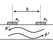
Figure 2. Two accelerometers placed on a beam, separated by distance Δ. These can be used to decompose the flexural propagating wave into two components.
Download figure:
Standard image High-resolution image


The wave decomposition operators given by equations (5a
) and (5b
) could be implemented directly in the frequency domain to decompose the acceleration signals into the incident and reflected wave components, however, this would only be suitable for use in a tonal control strategy. In this work, the aim is to implement a broadband control solution and, therefore, it is necessary to approximate the wave decomposition operators using broadband filters. This can be achieved in a digital control system by approximating H1 and H2 using finite impulse response (FIR) filters, as previously proposed in [42]. The accuracy of these filters is dependent on the filter length, sampling frequency and the spacing between the accelerometers [37, 38, 40, 42]. The filter impulse responses  and
and  can be found by taking the inverse Fourier transform of H1(ω) and H2(ω), however, to ensure that the impulse responses are causal, a modelling delay must first be added to H1(ω) and H2(ω) before approximating them as FIR filters [37]. This can be achieved by multiplying each frequency response by
  , so that the corresponding impulse response is an estimate of the wave amplitude ns
samples earlier [37, 40]. The effect of this delay on the performance of the control system can be reduced if the propagation time between the accelerometers and the control actuator is greater than ns
[39], but the introduction of this additional delay does deteriorate the control performance, particularly at higher frequencies [40]. Interestingly, the performance of a wave-based control system has been shown to be fairly robust to inaccuracies in the wave decomposition filter responses [37] and so a relatively small number of coefficients can be used in practice. The positive and negative propagating wave components can then be calculated in the discrete time domain via convolution between the FIR filters and the time domain accelerometer outputs as
, so that the corresponding impulse response is an estimate of the wave amplitude ns
samples earlier [37, 40]. The effect of this delay on the performance of the control system can be reduced if the propagation time between the accelerometers and the control actuator is greater than ns
[39], but the introduction of this additional delay does deteriorate the control performance, particularly at higher frequencies [40]. Interestingly, the performance of a wave-based control system has been shown to be fairly robust to inaccuracies in the wave decomposition filter responses [37] and so a relatively small number of coefficients can be used in practice. The positive and negative propagating wave components can then be calculated in the discrete time domain via convolution between the FIR filters and the time domain accelerometer outputs as
where a1(n) and a2(n) are the outputs of the two accelerometers at the nth time step.
2.1.1. Wave decomposition limitations.
As noted above, and previously discussed in [37, 40, 42], the wave decomposition approach described here is only accurate over a finite frequency range. At low-frequencies the accuracy of the wave decomposition is limited by the length of the filters,  and
and  , the sampling rate and the distance between the sensors and sources of near-field wave components [37, 40, 42]. In this investigation, due to the relatively compact nature of the system being considered, the low-frequency limit is related to the assumption that the near-field components can be neglected. The near-field waves have been considered negligible once they have decayed to 10% of their original value, which is consistent with the limits utilised in the ABH literature [2, 6], and this leads to the relation

This equation describes the decay of the evanescent wave amplitude over a distance of l, and can therefore be used to calculate the lowest frequency at which the near-field components have sufficiently decayed for a given spacing between the sensors and any sources of near-field wave components. For a rectangular beam section, the wavenumber can be calculated analytically as [36]
where ρ is the density of the material, E is the Young's modulus of the material and h is the height of the beam. By substituting equation (8) into equation (7) and re-arranging, the low frequency limit can be calculated as
The high frequency limit of the wave decomposition method is imposed by the sampling frequency, anti-aliasing filters and re-construction filters and the modelling delay used to design the wave decomposition filters,  and
and  . In addition, the spacing between the two sensors should be less than half the minimum wavelength of interest. These limits will be addressed in the context of this investigation in section 3.1.
2.2. Controller formulation
As noted above, the aim of the ABH terminated beam is to minimise the reflection coefficient and thus generate an anechoic termination. This has previously been achieved for a standard beam using a wave-based feedforward control strategy, as outlined in [37–40]. This strategy utilises the wave decomposition method described in section 2.1 to provide the positive and negative propagating wave components, the latter of which is used as the error signal in a feedforward control architecture. Figure 3 shows a block-diagram of the wave-based feedforward control system, which utilises the filtered-reference least mean squares (FxLMS) architecture.

Figure 3. A block-diagram showing a wave-based active control system. The digital controller,  , is adapted to minimise the error signal,
  .
.  is the disturbance signal that is measured at the accelerometer array,
  is an estimation of the plant response that is implemented as an FIR filter and
  is the filtered reference signal.
Download figure:
Standard image High-resolution imageThe wave-based feedforward control system considered here consists of a single control actuator, a pair of accelerometer error sensors, as described in section 2.1 and figure 2, and a reference signal, which in this case is provided by the signal driving the primary structural disturbance. As can be seen from the block-diagram shown in figure 3, the control filter,  , is adapted to minimise the error signal corresponding to the negative propagating wave,
  . This signal is obtained using the wave decomposition method described in section 2.1 and can be expressed following equation (6) as

where  and
and  are the wave decomposition FIR filters with Ih
coefficients and
are the wave decomposition FIR filters with Ih
coefficients and  and
and  are the vectors of current and past samples of the error signals measured at the two accelerometers mounted on the beam, as shown in figure 2, such that multiplication with the wave decomposition filter describes a convolution operation. The error signal vector corresponding to the lth sensor can be written as

The elements of this vector, which correspond to the signals measured at the lth sensor at the nth time step, can be expressed in terms of the summation of the disturbance signal at the sensor, dl (n), and the contribution due to the control signal, u(n), which operates via the secondary path, to give
where the secondary path between the control source and the lth error sensor has been represented by a Jth order FIR filter with coefficients glj
. As shown in figure 3, the control signal is generated by filtering the reference signal, x(n), via the control filter,  , which is implemented as an FIR filter with Iw
coefficients, wi
, which gives the control signal as
, which is implemented as an FIR filter with Iw
coefficients, wi
, which gives the control signal as
Substituting equation (13) into (12) then gives the error signal at the lth sensor as
and by making the assumption that the control filter is time-invariant [41], this can be rewritten as
where the reference signal filtered by the lth secondary path response is
Equation (15) can be more succinctly expressed using vector notation as

where

Following this same approach, the error signal corresponding to the negative propagating wave given by equation (10) can be expressed as

where  is the vector of current and past samples of the reference signal filtered by the plant response corresponding to the negative propagating wave and
  is the disturbance signal associated with the negative propagating wave. The individual elements of
  can be expressed using the wave decomposition filters as

where  in this case is the vector of the current and previous (Ih
−1) samples of the filtered reference signals described by equation (16). Similarly, the disturbance signal associated with the negative propagating wave can be expressed as
in this case is the vector of the current and previous (Ih
−1) samples of the filtered reference signals described by equation (16). Similarly, the disturbance signal associated with the negative propagating wave can be expressed as

where  is the vector of the current and previous (Ih
−1) samples of the disturbance signal at the lth sensor.
is the vector of the current and previous (Ih
−1) samples of the disturbance signal at the lth sensor.
With the error signal corresponding to the negative propagating wave expressed according to equation (19), it is possible to derive the optimal broadband control filter that minimises the cost function defined as the weighted summation of the mean-square error signal and the sum of the squared control filter coefficients. This cost function can be expressed as

where E denotes the expectation operator and β is a positive control effort coefficient-weighting parameter. The inclusion of the second term in the cost function has a number of practical benefits, as discussed in [41], however, it has been included here to enable a constraint to be imposed on the magnitude of the control signals. Substituting equation (19) into equation (22) gives the cost function as
The optimal vector of control filter coefficients can then be calculated by setting the derivative of equation (23) with respect to the control filter coefficients to zero and this leads to the optimal solution
which assumes that the inverted matrix is positive definite and can, therefore, be inverted. From equation (24) it can be seen that the control effort coefficient-weighting parameter, β, regularises the solution to the inverse problem, as discussed in [41]. It is relatively straightforward from this point to derive the adaptive version of the FxLMS algorithm that could be used to implement a controller with filter coefficients that converge towards the optimal solution given by equation (24), as described for example in [41]. However, in the following investigation the optimal solution given by equation (24) will be utilised to ensure that the limitations on the maximum control performance are clearly demonstrated.
3. Experimental investigation
In this section, an investigation into the optimum performance of an AABH is presented via a comparison with a standard beam with an active termination. In addition to the control performance, a comparison is also made in terms of the electrical power requirement and the computational demand, which governs the required DSP power. This section begins with a description of the experimental setup and this is followed by an investigation into the plant modelling requirements for the FxLMS controllers used by the two systems. The control performance for the two active terminations is then assessed via offline predictions using the measured responses and this is accompanied by a discussion of the results.
3.1. Experimental setup
The experimental setup used to investigate the performance of the AABH beam termination is shown in figure 4; an identical setup is used for the constant thickness beam termination. From this diagram it can be seen that the beams were instrumented with two accelerometers, which provide the error sensors for the wave decomposition described in section 2.1, and a single piezoelectric patch actuator, which provides the secondary control force, as utilised by the controller described in section 2.2. Piezoelectric materials have been widely employed in the active control of noise, vibration and flow, as reviewed in [43] and have previously been integrated with ABHs for energy harvesting applications [5, 44], but have not previously been used to combine active control with ABH structural features as proposed here. The control actuator in the study presented here was realised using a PI ceramic P-876.A11 piezoelectric patch actuator [45] and, as shown in figure 5, it was attached to the flat side of the ABH taper and to the end of the standard beam using adhesive; this arrangement avoids the introduction of different levels of pre-stress into the piezoelectric patch for the two beam terminations. The operating voltage range of the piezo patch is −50 to 200 V and the patch has a length of 61 mm, a width of 35 mm, a height of 0.4 mm and a mass of 2 g. The two accelerometers were positioned Δ = 2 cm apart and the centre point between them was located at lp = 21 cm from the primary disturbance, which was provided by a standalone shaker. By referring to the control system limits in section 2.1.1, the sensor placement gives a low frequency limit of approximately 400 Hz. The controller described in section 2.2 was implemented on a dSpace real-time rapid control prototyping system [46]. The sampling frequency of the control system utilised in the experimental setup was set to 24 kHz and the anti-aliasing low-pass filters were accordingly set to give a cut-off frequency of 10 kHz. The frequency range of this investigation was, therefore, limited to between 400 Hz and 10 kHz.
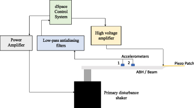
Figure 4. A diagram showing the experimental setup used to realise the active terminations for the AABH and standard constant thickness beam.
Download figure:
Standard image High-resolution image
Figure 5. Pictures of the experimental setup used to measure the responses of the beams with the ABH (a) and constant thickness (b) terminations.
Download figure:
Standard image High-resolution imageThe two beams, which are shown in the photographs of the two setups in figure 5, have been manufactured from a 10 mm thick sheet of aluminium alloy 6061-T6. Two identical beams, with a length of 370 mm and width of 40 mm, were cut from the sheet and then the ABH taper was cut into the end of one of the beams using a water jet cutter. The length of the ABH taper was set to 70 mm and based on the parametric design study presented in [6] was implemented with a power law of 4 and a tip height of 0.5 mm to maximise the passive performance of the taper. The dimensions of the two beams are summarised in table 1.
Table 1. The geometrical parameters of the beams with both an ABH and a constant thickness termination.
| Parameter | ABH termination | Constant thickness termination |
|---|---|---|
| Beam height (h(0)) | 10 mm | 10 mm |
Beam length ( ) ) | 300 mm | 370 mm |
| Beam width (b) | 40 mm | 40 mm |
Tip height ( ) ) | ∼0.5 mm | 10 mm |
Taper length ( ) ) | 70 mm | 0 mm |
| Taper power law (µ) | 4 | n/a |
3.2. Plant modelling
As shown in section 2.2, the proposed wave-based feedfoward active control system is implemented using the FxLMS algorithm and this requires an accurate model of the plant response to generate the filtered reference signal,  . The plant model is derived via a system identification procedure [47], where the response is first measured between the input to the control actuator and output from the error sensors and then approximated by an FIR filter model. To develop an understanding of the requirements of the plant model used to implement the controllers for the AABH and the active beam, a study that investigates how the plant modelling error varies with the number of filter coefficients in the plant model has been carried out.
In the first instance, the plant responses between the voltage input to the piezoelectric patch and the two accelerometers were measured for the two beams by driving the piezoelectric patch actuator with white noise, band-limited between 400 Hz and 10 kHz. The frequency responses were then calculated using the H1-estimator and corresponding FIR filters were calculated with between 10 and 5000 coefficients (or durations of between 0.4 and 200 ms at the 24 kHz sample rate) using the Matlab function invfreqz, which uses a least-squares approach based on [48]. The normalised mean-squared error (NMSE) between the modelled plant responses and the measured responses was then calculated for each filter length and averaged over both accelerometers as
where  is the column vector containing the frequency response of the identified plant and
  is the column vector containing the frequency response of the plant model FIR filter, both between the single control actuator and the lth accelerometer.
Figure 6 shows how the NMSE, calculated according to equation (25), decreases with increasing number of coefficients in the plant model FIR filter for both the AABH and constant thickness beam. From the results presented in figure 6 it can be seen that the AABH system requires fewer filter coefficients than the constant thickness active beam system to achieve the same NMSE in the plant model, or, alternatively, can achieve a lower level of NMSE for the same plant model filter length. This is a potentially significant advantage because it can be used to reduce the computational requirements of implementing the active feedforward control strategy outlined in section 2.2 on a DSP system. For example, in the case of the AABH if the plant model FIR filter was implemented with 400 coefficients the NMSE would be −28 dB, however, to achieve the same NMSE for the constant thickness beam termination would require 1430 FIR filter coefficients in the plant model. This means that the AABH termination potentially allows a more computationally efficient implementation of the FxLMS controller.
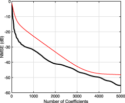
Figure 6. The NMSE between the frequency responses corresponding to the identified plant and the plant model FIR filters for an increasing number of FIR coefficients for the AABH (black thick line) and the constant thickness beam (thin red line).
Download figure:
Standard image High-resolution imageTo help explain why the standard beam termination requires a longer FIR filter to accurately model the plant response than that required by the AABH termination, figure 7 shows the magnitude of the identified plant frequency response for the two terminations. From the presented results it can be seen that the plant response for the constant thickness beam is characterised by three lightly damped resonances at 2.4, 3.7 and 7.8 kHz. These resonances significantly exceed the magnitude of any of the resonances present in the plant response for the AABH terminated beam and this is consistent with the expected passive performance of the AABH termination, which will be discussed further in section 3.3.2. It is worth noting that the passive damping is being provided here by the presence of the piezoelectric patch. The lightly damped resonances in the constant thickness beam will have an inherently slower decay rate than the resonances that characterise the AABH terminated beam and, therefore, require a longer FIR plant modelling filter.

Figure 7. The magnitude of the plant response measured between the voltage input to the piezoelectric patch actuator and the negative propagating wave generated by the actuator calculated according to equation (6) using the accelerations measured at the two accelerometers mounted on the beam section, as shown in figure 4, for the constant thickness beam (thin red line) and the AABH beam (black thick line).
Download figure:
Standard image High-resolution image3.3. Control performance
Having established the requirements in terms of the plant modelling filters for the two beam terminations in the previous section, this section will firstly investigate the requirements in terms of the control filter length for the two different configurations. Subsequently, a comparison between the broadband control performance for the two active terminations will be presented.
3.3.1. Control filter length.
To initially assess how many coefficients are required for the optimum control filter,  in figure 3, the total broadband averaged attenuation in the reflection coefficient has been calculated for a range of control filter lengths. The broadband averaged attenuation is defined as
where  is the reflection coefficient for the constant thickness beam without control averaged over frequency and
  is the reflection coefficient of the controlled system averaged over frequency. The broadband average attenuation was calculated using a range of between 0 and 500 control filter coefficients for both the AABH and constant thickness active beam terminations. The optimal control filter in each case has been calculated using equation (24) with the control effort weighting coefficient β set to zero for the AABH and, for the constant thickness beam configuration, set to constrain the peak-to-peak input voltage to be equal to that required to drive the piezoelectric patch actuator for the optimal AABH configuration. There are a variety of methods of selecting the regularisation parameter discussed in the literature, including Generalised Cross Validation [49], the L-curve method [50], and Morozov discrepancy principle [51]. However, the required value of β for the constant thickness beam configuration has been determined here by iteratively increasing β from zero until the peak-to-peak input voltage is equal to that required in the AABH configuration. This has been done to provide a direct comparison between the performance of the two system designs when they are each utilising the same electrical drive signal requirements. For each termination configuration, the plant model has been implemented to achieve the same NMSE, as defined by equation (25), such that the AABH implementation uses 400 coefficients and the standard active beam uses 1430 coefficients. Figure 8 shows for each of these cases the broadband average attenuation (a) and the maximum peak-to-peak input voltage to the piezoelectric actuator (b) for various control filter lengths.

Figure 8. The broadband averaged attenuation (a) and corresponding peak-to-peak voltage (b) for different configurations of the AVC termination with different control filter lengths. The thick black lines show the results for the AABH terminated beam, the thin red lines show the results for the constant thickness beam termination both without regularisation (dashed) and with regularisation to constrain the peak-to-peak voltage to match the requirements of the AABH (solid).
Download figure:
Standard image High-resolution imageFrom the results presented in figure 8(a), it can be seen that in all cases the broadband performance increases as the number of control filter coefficients is increased. The increase in broadband attenuation is initially quite rapid, however, for control filter lengths greater than 350 coefficients the broadband attenuation increases by less than 1 dB for all of the controllers. Therefore, in the following section the performance of the different beam terminations is compared for a control filter length of 350 coefficients. In addition to demonstrating how the performance varies with the number of control filter coefficients, figure 8(a) shows that the AABH provides more attenuation than either of the constant thickness beam configurations for the same control filter length up to 500 coefficients. This is because the AABH combines the performance of the active control system with the passive performance of the ABH. On this note, it is important to highlight that the AABH without control (i.e. when the control filter length is zero) achieves 4 dB more broadband attenuation than the constant thickness beam, which corresponds to the passive performance achieved via the ABH effect. For a control filter length of 500 coefficients, it can be seen from the results presented in figure 8(a) that the AABH and the unregularised constant thickness active beam termination achieve the same broadband attenuation. However, it is important to highlight using the results presented in figure 8(b), which show the maximum peak-to-peak voltage required by the controller in each case, that the constant thickness beam configuration requires almost 13 times the peak-to-peak voltage required by the AABH system. This means that the constant thickness beam configuration is less efficient than the AABH and, in practice, would require actuators and amplifiers rated to a significantly higher peak operating level. In fact, the peak-to-peak voltage required by the constant thickness beam configuration using the unregularised optimal control filter significantly exceeds the input voltage limits of the piezoelectric patch actuator utilised for this study. Therefore, the plots in figure 8 also show the performance when the optimal control filter solution for the constant thickness beam is regularised such that the required peak-to-peak voltage is equal to that required by the optimal AABH solution. In this case it can be seen that the AABH exceeds the broadband performance achieved by the regularised active constant thickness beam configuration by around 10 dB. It is important to note that this performance advantage is greater than that provided by the passive ABH effect alone, which provides a broadband attenuation of 4 dB. It is interesting to observe that a similar advantage was observed when combining active control elements with a Helmholtz resonator based metamaterial in [52] and the results presented here thus begin to demonstrate the advantage of the AABH termination compared to a constant thickness active beam termination.
3.3.2. Broadband performance.
To provide a more detailed comparison of the different active beam terminations, the broadband reflection coefficient for each termination has been calculated over frequency with and without control. The performance has also been calculated for the constant thickness active beam where the optimal control filter has been regularised to constrain the peak-to-peak input voltage to be equal to that required by the optimal AABH solution, therefore providing a consistent comparison between the two terminations for a practically realisable beam controller. Once again, the number of coefficients in the plant models has been set to give the same NMSE for both the AABH and the constant thickness beam termination and the number of coefficients in the control filter has been set to 350, based on the results presented in section 3.3.1. Figure 9 shows the resulting reflection coefficients and control effort, defined as  , required for each of the three controller configurations. In addition, the performance of an equivalent fully passive ABH termination has also been measured for reference, where the passive damping has been provided by a thin layer of viscoelastic material, as previously described in [6].

Figure 9. (a) The reflection coefficient of the AABH without control (solid black line) and with control using 400 coefficients in the plant model (dashed black line); the constant thickness active beam without control (solid red line), and with control using 1430 coefficients in the plant model both without regularisation (dashed red line) and with regularisation (dotted red line); and the passive ABH with a thin viscoelastic damping layer (thick blue line). In all active control cases the number of coefficients in the control filter is set to 350. (b) The control effort required in each control case with consistent line types. The control effort has been normalised so that a constant level at 0 dB corresponds to the maximum broadband input to the piezo.
Download figure:
Standard image High-resolution imageFigure 9(a) shows the reflection coefficient for the different beam termination configurations over frequency. From these results it is interesting to first highlight that the reflection coefficient for the constant thickness beam termination without control is close to 1 for most frequencies, while the reflection coefficient for the AABH without control features the bands of low reflection that are typical of a passive ABH termination; the passive damping in this case is being provided by the undriven piezoelectric patch. It is also interesting to compare the performance of the AABH without control to the performance of the passive ABH termination with a thin layer of viscoelastic damping applied to the taper. In this case it can be seen that the dips in the reflection coefficient are lower for the purely passive ABH than the uncontrolled AABH due to the greater level of damping provided by the viscoelastic material. It can also be seen that the nulls are shifted down in frequency compared to the uncontrolled AABH, which is in part due to the additional mass of the applied viscoelastic material (12 g) compared to the piezoelectric patch (2 g). These differences aside, it is clear that the passive ABH has limited low frequency performance and is relatively consistent in behaviour to the uncontrolled AABH.
From the active control results presented in figure 9(a) it can be seen that all three configurations (the AABH and the constant thickness beam with and without regularisation) achieve almost perfect control of the reflection coefficient above around 3 kHz. However, at lower frequencies it can be seen that the control performance shows some clear limitations for the three configurations. For the AABH it can be seen that the reflection control is limited at around 600 Hz, which corresponds to a dominant structural resonance that can be seen in the AABH plant response presented in figure 7. Similar limitations can also be seen for the constant thickness active beam termination, but occur at around 420 Hz, 1.1 kHz and 2.4 kHz, which correspond to significant structural resonances in the constant thickness beam response, as shown in figure 7. These peaks in the response largely account for the difference in the broadband averaged attenuation achieved by the unregularised active beam termination compared to the AABH, as shown in figure 8(a). Finally, it can be seen from the reflection coefficient for the regularised active beam configuration that the regularisation largely limits the control performance at frequencies below around 2 kHz and it is clear that the performance is comparable to the uncontrolled AABH.
Figure 9(b) shows the control effort for the three active configurations; the results in figure 9(b) are presented in decibels with reference to the control effort corresponding to the maximum broadband input to the piezoelectric actuator. From these results it can be seen that the unregularised constant thickness beam configuration requires up to 30 dB more control effort than the AABH and whilst this difference is largest at frequencies below around 2 kHz, the control effort requirements are notably larger even at higher frequencies. It can also be seen from the results presented in figure 9(b) that while the high levels of control effort that occur at low frequencies for the constant thickness beam termination are limited by the employed level of regularisation, the regularised constant thickness beam controller still requires a higher level of effort compared to the AABH at higher frequencies. These results demonstrate more clearly the advantages of the AABH termination over the constant thickness active beam termination that have already been noted in reference to the broadband averaged results presented in section 3.3.1. That is, the AABH is able to achieve improved control performance with a lower power requirement than the constant thickness active beam configuration. In addition, it is interesting to once again note that this enhanced performance goes beyond that provided by the passive ABH performance. That is, while the uncontrolled performance of this particular AABH is limited below around 1.2 kHz, the AABH with control is still able to achieve significant performance with a lower control effort than the constant thickness active beam configuration. This implies that the AABH not only offers the advantages of the additional passive performance, shown by the thin solid black line in figure 9(a), but also enables improved active control performance.
It is has been shown by the presented results that the AABH is able to outperform the constant thickness active beam termination in terms of the broadband attenuation in the reflection coefficient. It has also been shown that the control efficiency of the AABH is greater than the constant thickness active beam termination, with the AABH requiring a significantly reduced control effort. The AABH thus offers a number of advantages over the constant thickness active beam termination, however, it is interesting to also understand how the AABH influences the response of the termination section of the beam. Therefore, figure 10 shows the response measured at the centre of the termination section both with and without control for the AABH and constant thickness active beam terminations. By comparing the uncontrolled responses in figures 10(a) and (b) it can be seen that, on average, the uncontrolled AABH response is around 10 dB greater than the response of the constant thickness beam termination. This result is as expected given the reliance of the ABH effect on focusing energy into the taper, as previously observed for passive ABHs [11, 17, 23]. However, it is interesting to observe here the effect of control on the response of the two different terminations and it can be seen from the presented results that the AABH significantly enhances the response in the termination section across the majority of the presented bandwidth, whereas the constant thickness active beam termination introduces relatively modest variations in the response, with the main enhancement occurring between 3 and 5 kHz where the uncontrolled response is low. These results indicate that it is clearly important when considering the practical utilisation of the AABH to consider the trade-off between enhancing the stress concentration in the taper and improving the vibration control of the structure overall, as considered for passive ABHs in [44]. Further work is clearly required to investigate this trade-off for the AABH.
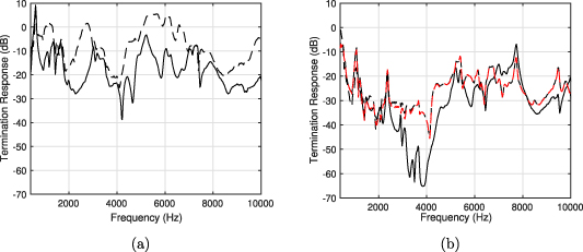
Figure 10. The response measured at the centre of the termination section for (a) the AABH without control (solid line) and with control (dashed line); and (b) the active beam without control (solid line) and with control (dashed lines) without regularisation (red) and with regularisation (black).
Download figure:
Standard image High-resolution image4. Real-time experimental validation
In this section, in order to validate the practicability of the systems investigated in the previous section via offline predictions using measured responses, the performance achieved by real-time experimental implementations is presented for both the AABH and the constant thickness active beam termination. The plant models for the two configurations have again been set to give the same NMSE, with 400 coefficients used for the AABH plant model and 1430 coefficients used for the constant thickness beam termination. In both cases, 350 coefficients have been used in the control filters, as defined according to the investigation presented in section 3.3.1, and the optimal control filters have been calculated using equation (24). Due to the practical limits of the piezoelectric actuator, it is not possible to experimentally evaluate the unconstrained constant thickness active beam configuration and, therefore, the results are only presented for the AABH and the constant thickness active beam with regularisation set so that the peak-to-peak voltage is consistent with that required by the optimal AABH configuration.
Figure 11(a) shows the reflection coefficient measured both with and without control for the constant thickness active beam termination and the AABH; the corresponding control efforts are shown in figure 11(b). From these results it can be seen that the real-time results are consistent with the results of the offline predictions presented in section 3.3.2. It is once again clear that the AABH outperforms the regularised constant thickness active beam termination in terms of the control achieved in the reflection coefficient, whilst requiring the same peak-to-peak drive voltage. The control effort also shows the same trend observed in section 3.3.2, with the active beam requiring a generally higher level of control effort, except most notably at frequencies below around 1 kHz where the regularisation used in the active beam termination limits the requirements. A general observation that can be made in comparing the real-time measurements to the offline results presented in figure 9, is that the peaks in the controlled responses, which are most noticeable for the standard beam termination, are more significant in the real-time results. These peaks in the reflection coefficient are related to the rapid phase change associated with lightly damped resonances in the structure leading to narrowband errors between the plant model and the physical plant; the effects of this are exacerbated in the real-time results due to finite precision effects. Despite these narrowband differences between the predictions and measurement results, the broadband reflection coefficient differs by only 0.1 in the case of the constant thickness beam results and 0.06 in the case of the AABH, therefore demonstrating that the offline predictions provide a reliable estimation of the real-time performance. Nevertheless, it is clear from the real-time results presented in figure 11 that the AABH offers potentially significant advantages in terms of control performance compared to the constant thickness active beam termination.

Figure 11. (a) The reflection coefficient of the AABH without control (solid black line) and with control using 400 coefficients in the plant model (dashed black line), and the standard active beam without control (solid red line), and with regularised control using 1430 coefficients in the plant model (dotted red line). (b) The control effort required in each control case with consistent line types. The control effort has been normalised so that a constant level at 0 dB corresponds to the maximum broadband input to the piezo.
Download figure:
Standard image High-resolution image
5. Conclusions
This paper has proposed and presented an investigation into the AABH, which combines the ABH effect with active control technology in order to enhance the achievable levels of vibration control via a smart structure. An AABH beam termination has been described, in which a single piezoelectric patch actuator is applied to the tapered ABH termination and driven to minimise the flexural wave reflected from the beam termination. The characteristic behaviour of the AABH termination has then been compared to a constant thickness active beam termination, which does not feature the tapering thickness profile of the ABH.
In the first instance, the presented comparison has demonstrated that the plant model required by the feedforward wave-based active control strategy can be implemented with less filter coefficients for the AABH than for the constant thickness active beam termination. This means that the AABH can be implemented with a lower computational requirement than the constant thickness active beam termination, whilst achieving the same level of NMSE in the plant model. In terms of the control performance, it has been shown through both offline predictions using measured responses and through real-time implementations, that the AABH termination is able to achieve a higher level of reflection control, whilst requiring a generally lower level of control effort. This means that the AABH can be implemented using hardware with a lower power rating and, therefore, lower cost than that required by the constant thickness active beam termination to reach the same level of control performance.
When the AABH and constant thickness active beam terminations are constrained to use the same peak-to-peak control voltage, it has been shown that the AABH provides a 10 dB broadband control performance advantage for the considered configuration. It has also been shown that this performance advantage is significantly greater than the level of control provided by the passive ABH effect alone, which is 4 dB for the investigated configuration. Therefore, the AABH offers a performance advantage above that expected from simply combining the levels of control offered by the constant thickness active beam termination and the ABH effect. Finally, the effects of active control on the response within the beam terminations has been investigated and it has been shown that the AABH significantly enhances the vibration in the termination compared to the constant thickness active beam configuration. This has been linked to the focusing effect observed in passive ABHs and it has been highlighted that the resulting structural fatigue issues should be considered when applying the AABH in practice.
This paper has focused on the realisation and evaluation of a one-dimensional AABH to a beam. In other work, the passive ABH concept has been extended to two-dimensional structures, such as plates, by rotating the one-dimensional taper by 360∘ to form a power law pit or dish, as described for example in [11, 13, 17, 20]. The AABH concept can potentially be extended to a two-dimensional ABH through the integration of an appropriate actuator, such as a circular piezoelectric patch actuator and a wider distribution of sensors. However, it is anticipated that a modified control strategy compared to that proposed in this paper would be required since the concept of reflection control does not readily extend to a two-dimensional structure, such as a plate. It is proposed that a more viable approach would result if the controller instead aimed to control a proxy for the kinetic energy in the plate, such as the sum of the squared velocities measured at a number of structural sensors.
Acknowledgment
This work was supported by an EPSRC iCASE studentship (Voucher Number 16000058) and the Intelligent Structures for Low Noise Environments (ISLNE) EPSRC Prosperity Partnership (EP/S03661X/1).