
Abstract
The use of superconducting wire within AC power systems is complicated by the dissipative interactions that occur when a superconductor is exposed to an alternating current and/or magnetic field, giving rise to a superconducting AC loss caused by the motion of vortices within the superconducting material. When a superconductor is exposed to an alternating field whilst carrying a constant DC transport current, a DC electrical resistance can be observed, commonly referred to as 'dynamic resistance.' Dynamic resistance is relevant to many potential high-temperature superconducting (HTS) applications and has been identified as critical to understanding the operating mechanism of HTS flux pump devices. In this paper, a 2D numerical model based on the finite-element method and implementing the H-formulation is used to calculate the dynamic resistance and total AC loss in a coated-conductor HTS wire carrying an arbitrary DC transport current and exposed to background AC magnetic fields up to 100 mT. The measured angular dependence of the superconducting properties of the wire are used as input data, and the model is validated using experimental data for magnetic fields perpendicular to the plane of the wire, as well as at angles of 30° and 60° to this axis. The model is used to obtain insights into the characteristics of such dynamic resistance, including its relationship with the applied current and field, the wire's superconducting properties, the threshold field above which dynamic resistance is generated and the flux-flow resistance that arises when the total driven transport current exceeds the field-dependent critical current, Ic(B), of the wire. It is shown that the dynamic resistance can be mostly determined by the perpendicular field component with subtle differences determined by the angular dependence of the superconducting properties of the wire. The dynamic resistance in parallel fields is essentially negligible until Jc is exceeded and flux-flow resistance occurs.
Export citation and abstract BibTeX RIS

Original content from this work may be used under the terms of the Creative Commons Attribution 3.0 licence. Any further distribution of this work must maintain attribution to the author(s) and the title of the work, journal citation and DOI.
1. Introduction
Recent advances in the manufacturing of high-temperature superconducting (HTS) wire mean that long lengths (km+) of 'coated-conductor' ReBCO wire are now commercially available. This has sparked new interest in a range of new large-scale applications for superconducting magnets and power systems, which exploit the higher operating temperatures and associated thermal 'robustness' inherent to HTS materials. In particular, the development of AC power system applications, such as transformers, motors and generators, is an area of expanding interest.
However, the use of superconducting wire within an AC power system is complicated by the dissipative interactions that occur when a superconductor is exposed to an alternating current and/or magnetic field. This gives rise to a superconducting AC loss, caused by the motion of vortices within the superconducting material: 'magnetisation loss' describes dissipation due to the purely magnetic hysteresis behaviour of a superconducting body carrying zero transport current and 'transport loss' describes dissipation which occurs when an alternating transport current imposes an alternating self-field on a conductor, in the absence of an applied field. In practical applications, a cryogenic cooling system must extract the resulting heat load in order to enable constant temperature operation, and this means a comprehensive understanding of the mechanism and magnitude of AC losses is extremely important to the design and development of new superconducting magnets and rotating machines.
AC loss also arises when a superconductor is exposed to an alternating field whilst carrying a constant DC transport current. In this case, a DC electrical resistance is observed, commonly referred to as 'dynamic resistance' [1–4]. This situation is relevant to many potential HTS applications, including superconducting synchronous machines, NMR magnets and other unshielded DC magnet applications, and this dynamic resistance been identified as critical to understanding the operating mechanism of HTS flux pump devices [5–9]. Dynamic resistance, Rdyn, can be measured using simple electrical techniques, and gives rise to a dissipative loss Qdyn = Idc2Rdyn, where Idc is the DC transport current. However, in this situation, there also exist simultaneous magnetisation losses within the wire that are not probed by this particular electrical measurement. The total loss is a combination of the dynamic resistance and magnetisation terms, and is difficult to measure experimentally, due to additional dissipation associated with the DC current injection.
In this paper, a 2D numerical model based on the finite-element method and implementing the H-formulation is used to calculate the dynamic resistance and total AC loss in a coated-conductor HTS wire carrying an arbitrary DC transport current and exposed to background AC magnetic fields up to 100 mT. The measured angular dependence of the superconducting properties of wire, Ic(B, θ), and n-value, n(B, θ), for the E–J power law representing the superconductor's electrical resistivity, are used as input data, and the model is validated using measured experimental data for external AC magnetic fields applied perpendicular to the plane of the wire, as well as at angles of 30° and 60°. The model is used to obtain insights into the particular characteristics of such dynamic resistance, including its relationship with the applied current and field, the superconducting properties of the wire, the threshold field above which dynamic resistance is generated and the flux-flow resistance that arises when the total driven transport current exceeds the field-dependent critical current, Ic(B), of the wire.
1.1. Numerical modelling framework
The 2D infinitely long numerical model, shown in figure 1, is based on the H-formulation [10–16], where the governing equations are derived from Maxwell's equations: Faraday's law (1) and Ampere's law (2).


where H = [Hx, Hy] represents the components of the magnetic field strength, J = [Jz] represents the current density and E = [Ez] represents the electric field. μ0 is the permeability of free space, and for the superconducting layer and surrounding sub-domain (simply assumed to be air), the relative permeability is simply μr = 1. Only the superconducting layer of the wire is modelled, assuming that eddy current losses within the wire architecture (e.g., substrate, stabiliser layers) is negligible: a reasonable assumption for the wire at power frequencies (∼50/60 Hz) [17, 18]. Since the substrate of the wire under investigation is non-magnetic, consideration of any ferromagnetic losses, and indeed the influence of a magnetic substrate on the superconducting properties, is also unnecessary. Isothermal conditions are assumed and a constant temperature, T = 77 K; hence, no thermal model is included.
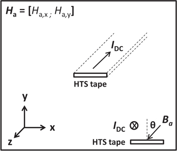
Figure 1. 2D infinite long numerical model geometry used to calculate the dynamic resistance of the HTS coated-conductor wire. The instantaneous external AC magnetic field applied to the wire at frequency f is Ba(t) = Bapp·sin(2πft). IDC is the DC transport current flowing along the wire. Ha,x, Ha,y are the Cartesian components of Ha = Ba/μ0.
Download figure:
Standard image High-resolution imageIt is assumed that electric field Ez is parallel to the current density Jz and the electrical properties of the superconductor are modelled by the E–J power law [19, 20] in (3).

where E0 is the characteristic electric field, 1 μV cm−1, B is magnitude of the local magnetic flux density and θ is the angular direction of that field as defined in figure 1.
Traditionally, the relationship between the critical current density Jc(B, θ) and the critical current Ic(B, θ) is given by (4), where S is the cross-sectional area of the superconducting layer. However, this direct approach does not include self-field effects, i.e., B refers to the external applied field, rather than the local magnetic flux density in (3). This can introduce numerical errors when the applied field is comparable to the self-field. Since, in this paper, the applied fields are 100 mT or less, the self-field is taken into account when calculating Jc(B, θ) based on the technique presented in [21], and using the example model files available at [22], which obtains Jc(B, θ) based on the local magnetic flux density, rather than the external applied field using (4). The width of the tape is 4 mm and the thickness of the superconducting layer is 1 μm; however, the homogenisation technique presented in [23, 24] is used to improve the computational speed of the model without compromising accuracy, and the thickness of the superconducting layer in the model is artificially expanded to 100 μm.

Experimentally measured values of Ic(B, θ) (from which Jc(B, θ) is calculated as described above) and n(B, θ) were used in the H-formulation model. This data was obtained at 77 K in magnetic fields up to 0.5 T, from a short sample of the same SuperPower SCS4050-AP wire as used in our dynamic resistance experiments. The experimental values, shown in figures 2 and 3, respectively, are input into the model using a two-variable, direct interpolation [25, 26], which is significantly faster than data fitting methods, yet without compromising accuracy. The measured, self-field critical current, Ic0, of the wire at 77 K is 107.5 A. In figure 3, there is some scatter in the calculated n-values after fitting equation (3) to the experimental data, most noticeable for the 0 T data where a scatter of n ± 2–3 is observed. The n-value fit is sensitive to the curvature of the experimental data above Jc, a regime where the experimental data is also vulnerable to the influence of resistive heating. However, at higher fields, this scatter is substantially depressed and the systematic 'double-peak' in the n-value is clear, following the measured Ic data in figure 2.
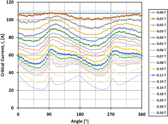
Figure 2. Experimental Ic(B, θ) data used in the H-formulation model. Data was measured at 77 K in magnetic fields up to 0.5 T from a short sample of SuperPower's SCS4050-AP wire. The Jc(B, θ) data is corrected for self-field using the technique presented in [21] and input into the model using a two-variable, direct interpolation [25, 26].
Download figure:
Standard image High-resolution image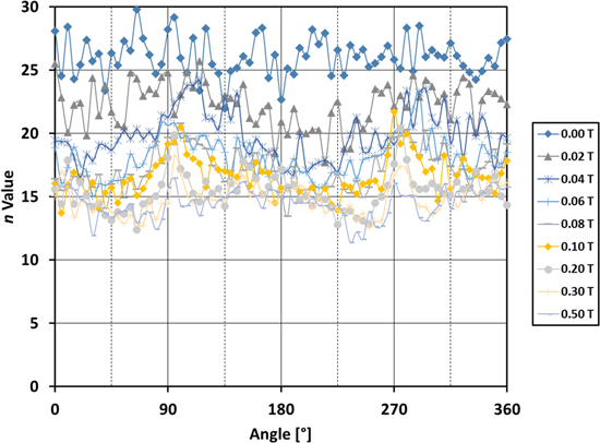
Figure 3. Experimental n(B, θ) data used in the model, measured at 77 K in magnetic fields up to 0.5 T from a short sample of SuperPower's SCS4050-AP wire. The data is input into the model using a two-variable, direct interpolation [25, 26].
Download figure:
Standard image High-resolution imageA mapped mesh (200 x-elements along the width, 10 y-elements along the thickness, and a linear element distribution with an element ratio of 3 between the central elements and the edge and top/bottom surface elements) is used in the superconducting layer to decrease the number of mesh elements [27], while still retaining enough mesh elements at the top and bottom of the wire to accurately simulate the current density associated with the DC current, and a free triangular mesh is used in the surrounding sub-domain. Linear, curl-conforming elements are employed for the entire model. For the non-superconducting sub-domain surrounding the superconducting layer, a linear Ohm's law is considered, E = ρJ, where ρ = 1 Ω m is a specific, high constant resistivity.
An integral constraint is applied to the superconducting layer to represent the DC transport current flowing in the superconducting tape. A transport current, I, through the cross-section S of the tape is therefore described by (5).

where Iapp(t) is a ramp function of ramp rate 10 A s−1 that is then held at its final value, IDC, which is defined by the ratio of IDC/Ic. In this paper, the cases for IDC/Ic = 0.3, 0.5, 0.7 and 0.9 are examined, where Ic = 107.5 A as defined earlier.
Once the appropriate IDC/Ic value is reached, AC magnetic fields up to 100 mT in amplitude are applied in 5 mT increments by setting appropriate boundary conditions for Hx, Hy [28]: the instantaneous external AC magnetic field applied to the wire at frequency f is Ba(t) = Bapp·sin(2πft), and Ha,x, Ha,y are the Cartesian components of Ha = Ba/μ0, as shown in figure 1. As such both θ = 0° and θ = 180° are perpendicular to the plane of the wire, but point in opposite directions, i.e., into top surface and substrate side of the wire, respectively.
The calculation of the total AC loss (J m−1/cycle) includes separate contributions from the magnetisation loss, Qmag, and the dynamic resistance, Qdyn, and in the 2D infinitely long model of the superconducting tape, this can be expressed as (6).
where T is the period of one cycle. When computing this value, we have taken the integral result between 0.5 T and 1.5 T, as this period does not include the transient, first half-cycle, where the superconductor is magnetised from its 'virgin' state [29].
In order to calculate the dynamic resistance, the average electric field across the entire conductor cross-section is firstly obtained using (7). The instantaneous dynamic resistance and associated power loss can then be obtained from (8) and (9), respectively, and the dynamic resistance loss, Qdyn, can be calculated from (10). Finally, the dynamic resistance, Rdyn, in units of (Ω m−1/cycle) can be found using (11).


This approach removes ambiguity in defining the geometric boundaries between the transport and magnetisation currents throughout the AC cycle, and hence differs from previous analytical and finite-element approaches, which have considered dynamic resistance to arise only from current flowing in the central region of the wire [30–32].
1.2. Experimental setup
A detailed description of the experimental procedure for the dynamic resistance measurements can be found in [33]. An AC magnetic field was applied by a copper-wound electro-magnet that can generate up to 100 mT peak magnetic field at frequencies up to 112.5 Hz [34]. The sample can be rotated inside the magnet, and the field angle, θ, can thus be varied. A DC power supply was used to supply a DC transport current of up to 300 A to the SuperPower sample. Two voltage taps were soldered on the edges of the sample, and the leads were arranged in a spiral loop to minimise induced AC pick-up from the external magnetic field [35]. The distance between the voltage taps in these experiments was 5 cm and the time-averaged DC voltage across the voltage taps was measured using a Keithley 2182 nano-voltmeter.
2. Model verification and experimental results
2.1. Perpendicular applied magnetic fields
2.1.1. Total AC loss
Firstly, the magnetisation AC loss of the wire is calculated for the case where the DC transport current is zero and an external AC magnetic field is applied perpendicular to the plane of the wire, i.e., θ = 0°. Figure 4 shows the calculated magnetisation AC loss, normalised by ∣Bapp∣2 (where Bapp = μ0Happ), of the wire for magnetic fields up to 100 mT and for frequencies of 20, 50 and 100 Hz, as calculated by the numerical model and compared with Brandt's analytical equation [36]. It is shown that the numerical model calculation is slightly higher than the analytical result due to our use of measured, real Jc(B) characteristics, rather than the constant Jc approximation used in the Brandt equation. There is also a slight frequency dependence of the simulation result, which is commonly observed when using time-dependent models based on the E–J power law [37–40]. The impact of this on the dynamic resistance calculations is discussed later in the paper. Despite these minor discrepancies, values calculated using equation (6) are broadly consistent with the Brandt expression, thus validating our numerical model. This also gives a base case to compare subsequent total AC loss calculations in which a DC transport current gives rise to loss components from both magnetisation loss and dynamic resistance.
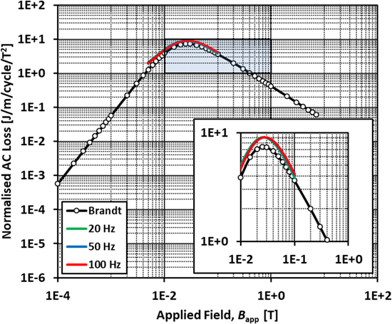
Figure 4. Comparison of calculated magnetisation AC loss using the numerical model for perpendicular magnetic fields up to 100 mT and analytical results according to the Brandt equation [36]. The analytical calculation uses Jc0 = 2.6875 × 10¹⁰ A m−2, which corresponds to the measured Ic (77 K, self-field) = 107.5 A and a width of 4 mm and thickness 1 μm for the superconducting layer. The results are normalised with respect to ∣Bapp∣2.
Download figure:
Standard image High-resolution imageThe maxima of the normalised magnetisation AC loss in figure 4 correspond to the effective penetration field of the wire, as it denotes the point at which the shielding current capacity is effectively saturated [30]. For values of IDC > 0, the maxima shift due to the superposition of the transport current and shielding (magnetisation) currents, with the effective penetration field decreasing with increasing values of IDC. This is shown clearly in figure 5. As in the zero current case, these maxima similarly correspond to the threshold field, Bth, above which where there is no longer a shielded region inside the wire and hence dynamic resistance occurs. For the case IDC/Ic = 0.9, there are also minima turning points, such that for fields above these points, the normalised total AC loss begins to increase again. This relates to the emergence of an additional flux-flow resistance term that arises once the total driven transport current exceeds the field-dependent Ic of the wire [30]. In the following section, the relationship of these maxima and minima present in the total AC loss curves and the particular characteristics of the dynamic resistance curves are explained in more detail.
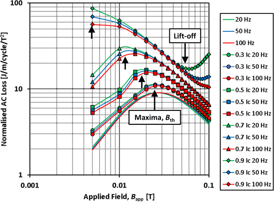
Figure 5. Calculated total AC loss, which includes the contribution of the magnetisation loss, Qmag, and the contribution from the dynamic resistance, Qdyn, as described by (6), using the numerical model for perpendicular magnetic fields up to 100 mT and DC transport currents corresponding to IDC/Ic = 0.3, 0.5, 0.7 and 0.9. The case from figure 4 when no DC transport current is applied, i.e., IDC/Ic = 0, is also shown for comparison. The results are normalised with respect to ∣Bapp∣2.
Download figure:
Standard image High-resolution image2.1.2. Dynamic resistance
In this section, the dynamic resistance is calculated using the numerical model based on (7)–(11). Figure 6 shows the calculated average electric field, using (7), across the cross-section of the wire for 0.5Ic under perpendicular external AC magnetic fields with ∣Bapp∣ = 20, 40, 60, 80 and 100 mT (middle); and 0.9 Ic for ∣Bapp∣ = 20, 40, 50 and 60 mT (bottom). The data from such waveforms can then be transformed using (8)–(11) to calculate the dynamic resistance in (Ω m−1/cycle). Interestingly, figure 6 shows that dynamic resistance is incurred when d∣Ba(t)∣/dt is largest, i.e., in the region around Ba(t) = 0. In contrast, flux-flow resistance manifests itself as a spike in the voltage when d∣Ba(t)∣/dt is lowest, i.e., at the maxima and minima of the applied field, ±Bmax. Additionally, there is some noticeable asymmetry of the voltage between positive and negative half-cycles of the applied field. This is related to the angular dependence of the superconducting properties of the wire (see figures 2 and 3), which differs slightly depending on whether the field is oriented towards the top surface (θ = 0°) or bottom surface (substrate side; θ = 180°). For the wire studied here (for fields up to 100 mT), we see that Jc(B, θ = 180°) tends to be slightly lower than Jc(B, θ = 0°).
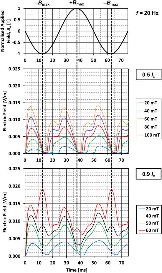
Figure 6. Calculated average electric field across the cross-section of the wire for 0.5Ic for perpendicular external AC magnetic fields with amplitude ∣Bapp∣ = 20, 40, 60, 80 and 100 mT (middle figure); and 0.9Ic for ∣Bapp∣ = 20, 40, 50 and 60 mT (bottom figure) for a frequency of 20 Hz. The top figure shows the normalised Ba(t) with time, where +Bmax corresponds to the peak of the applied field oriented towards the top surface (θ = 0°) and −Bmax corresponds to the peak of the applied field oriented towards the bottom surface (substrate side; θ = 180°).
Download figure:
Standard image High-resolution imageFigure 7 shows a comparison of the calculated dynamic resistance per cycle with the experimental results for IDC/Ic = (a) 0.3, (b) 0.5, (c) 0.7 and (d) 0.9 under applied perpendicular magnetic fields up to 100 mT (in 5 mT increments). The numerical results are calculated for frequencies of 20, 50 and 100 Hz whilst the experimental results correspond to frequencies of 26.62, 65.44 and 112.5 Hz. In figure 7(d), the calculated results using the analytical equations presented in [30] are also included (closed symbols), which takes into account the flux-flow resistance term that arises once the total driven transport current exceeds the field-dependent Ic of the wire. This effect gives rise to a nonlinear 'lift-off' from the constant value of dRdyn/d∣Bapp∣ observed at lower fields. The modelling results show excellent qualitative agreement with the experimental results and very good quantitative agreement, especially with respect to Bth (the threshold field above which Rdyn is generated) and the slope of Rdyn. Three important points to make are: (a) the calculated values exhibit a small frequency dependence of the slope, dRdyn/d∣Bapp∣, due to the use of the E–J power law (as described earlier with reference to the AC loss results shown in figures 4 and 5); (b) isothermal conditions are assumed with a constant temperature, T = 77 K, so this ignores any temperature increase that might occur due to heat dissipation (in particular when the Jc of the wire is exceeded resulting in the 'lift-off' regime); and (c) the wire is assumed to have uniform properties across the entire cross-section (and along the length, which is a necessary condition for the 2D infinitely long approximation). Real wires do not entirely meet this criteria, and this can influence the DC and AC properties of an HTS coated-conductor wire [31, 41, 42]. In principle such information could also be implemented in the model to improve the modelling assumptions, as shown in [40]. Nevertheless, the numerical model developed here now provides a useful and flexible tool to predict the characteristics of dynamic resistance generated in any HTS coated-conductor wire for which the relevant geometric and superconducting properties are known, as well as more complicated arrangements of such wires, such as multiple-wire stacks [43], cables and so on.

Figure 7. Comparison of the calculated dynamic resistance and experimental results for IDC/Ic = (a) 0.3, (b) 0.5, (c) 0.7 and (d) 0.9 for perpendicular external AC magnetic field amplitudes up to 100 mT (in 5 mT increments). The results are calculated for frequencies of 20, 50 and 100 Hz and the experimental data corresponds to frequencies of 26.62, 65.44 and 112.5 Hz.
Download figure:
Standard image High-resolution imageIn figure 5, the AC loss maxima are indicated for each DC transport current case. These correspond to the threshold field, Bth, below which it is energetically favourable for the central region of the wire to be shielded from changes in the applied field [30]. When Bth is exceeded, dynamic resistance is incurred and increases linearly with ∣Bapp∣. Using the numerical model, it is easy to visualise this effect, through mapping the current density distribution within the wire cross-section for different regimes under a perpendicular external AC magnetic field. Figure 8 shows the calculated current density distribution, normalised by Jc(B) (where B is the local magnetic flux density), for the simple DC transport current cases (in the absence of an applied AC field) at the time when the ramped current reaches its final value, IDC/Ic. Figure 9 then shows the normalised, calculated current density distribution, which arises under a perpendicular external AC magnetic field when IDC = 0.3Ic, for ∣Bapp∣ = 10 mT (figure 9(a)) and 60 mT (figure 9(b)). The distributions are shown at the positive and negative peaks of the applied field, as well as the zero-crossing (f = 20 Hz). Figure 9(a) corresponds to Rdyn = 0 in figure 7(a), and shows the superposition of the transport current and magnetisation currents (with respect to figure 8). It clearly shows a shielded central region that does not experience a change in applied field, and for which J = 0. In contrast, figure 9(b) shows the situation when the central region is no longer shielded throughout the entire cycle, such that J ≥ Jc at all points within the wire, except for a very thin boundary region in which the current reverses direction. The result in this case is that a net flow of flux crosses the DC current-carrying region [4], leading to the development of Rdyn.
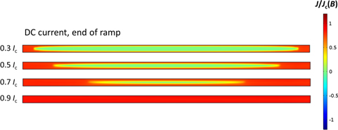
Figure 8. Calculated current density distributions, normalised by Jc(B), within the cross-section of the wire for the simple DC transport current cases (in the absence of an applied AC field) at the time when the ramped current reaches its final value as defined by IDC/Ic.
Download figure:
Standard image High-resolution image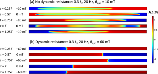
Figure 9. Calculated current density distributions, normalised by Jc(B), within the cross-section of the wire for perpendicular external AC magnetic fields when IDC = 0.3Ic and f = 20 Hz. Data is shown for the instants at the positive and negative peaks of the applied field, as well as the zero-crossing. Two cases are shown: (a) ∣Bapp∣ = 10 mT and (b) ∣Bapp∣ = 60 mT.
Download figure:
Standard image High-resolution imageIn contrast, figure 10 shows the normalised current density distribution, J/Jc(B) when IDC = 0.9Ic for ∣Bapp∣ = 30 mT (figure 10(a)) and 60 mT (figure 10(b)). As before, the distributions are shown at the positive and negative peaks of the applied field, as well as the zero-crossing (f = 20 Hz). The top figure corresponds to the linear regime (no shielded region and ±Jc current-carrying regions). The bottom figure corresponds to the 'lift-off' regime (see figure 7(d)), where there exists an additional flux-flow resistance term because the total driven transport current exceeds the field-dependent Ic of the wire. This 'lift-off' also results in the minima observed in the calculated total AC loss (see figure 5) and the development of a 'spike' in the calculated average electric field (see figure 6) around the peak of ∣Bapp∣, which is in clear contrast to figure 6 (middle), where the average electric field is close to zero around the peak of ∣Bapp∣.
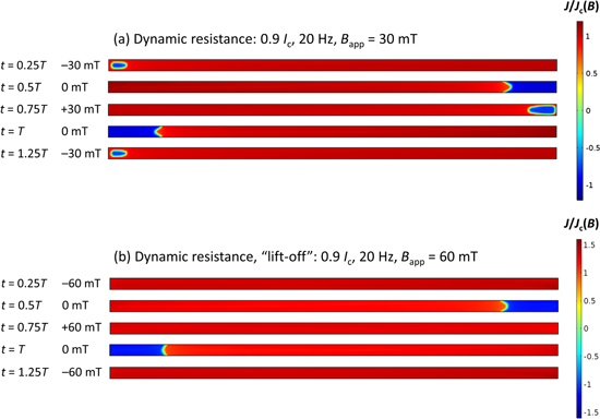
Figure 10. Calculated current density distributions, normalised by Jc(B), within the cross-section of the wire for perpendicular external AC magnetic fields when IDC = 0.9Ic and f = 20 Hz. Data is shown for the instants at the positive and negative peaks of the applied field, as well as the zero-crossing. Two cases are shown: (a) ∣Bapp∣ = 30 mT and (b) 60 mT. Case (a) corresponds to the linear dynamic resistance regime, and case (b) corresponds to the 'lift-off' regime, where there exists an additional flux-flow resistance term because the total driven transport current exceeds the field-dependent Ic throughout the wire. Note the different scale used in (b), where the current density J significantly exceeds the Jc of the wire.
Download figure:
Standard image High-resolution image2.2. Angular dependence of dynamic resistance: θ = ±30°, ±60°
The flexibility of the numerical model and the inclusion of the full angular dependence of the superconducting properties of the wire allows us to simulate the angular dependence of the dynamic resistance over the full range of applied field angles. Recent experimental measurements on a similar wire presented in [31] have shown that the dynamic resistance is dominated by the perpendicular magnetic field component, with negligible contribution from the parallel component. Figure 11 shows a comparison of the calculated dynamic resistance and experimental results for IDC/Ic = (a) 0.3, (b) 0.5, (c) 0.7 and (d) 0.9 for magnetic fields up to 100 mT (in 5 mT increments and f = 20 Hz (simulation) and 26.62 Hz (experiment)) applied perpendicularly and at angles of θ = −30° and −60°. These results are plotted as a function of the amplitude of the perpendicular component of the applied magnetic field, Bapp,⊥ = Bapp · cos(θ). This clearly shows that the dynamic resistance is dominated by the perpendicular component of the applied magnetic field, with some subtle differences: for θ = −60°, the slope dRdyn/d∣Bapp,⊥∣ is slightly higher and 'lift-off' occurs at a lower value of ∣Bapp,⊥∣.

Figure 11. Comparison of the calculated dynamic resistance and experimental results for IDC/Ic = (a) 0.3, (b) 0.5, (c) 0.7 and (d) 0.9 for external AC magnetic field amplitudes up to 100 mT (in 5 mT increments and f = 20 Hz (simulation) and 26.62 Hz (experiment)) applied perpendicularly and at angles of θ = −30° and −60°. The results are plotted as a function of the amplitude of the perpendicular component of the applied magnetic field, Bapp,⊥ = Bapp · cos(θ).
Download figure:
Standard image High-resolution imageTo explain these subtle differences and to obtain a complete picture of the dynamic resistance of the wire, figure 12 shows a comparison of the angular dependence of the calculated dynamic resistance and experimental results for IDC/Ic = (a) 0.3, (b) 0.5, (c) 0.7 and (d) 0.9 for magnetic fields up to 100 mT (in 5 mT increments) applied at an angle of θ = ±30°, and figure 13 shows the same plots, but for an applied field angle of θ = ±60°. The numerical results are calculated for frequencies of 20, 50 and 100 Hz and the experimental results correspond to frequencies of 26.62, 65.44 and 112.5 Hz. The modelling results show excellent qualitative agreement with the experimental results and very good quantitative agreement, with the same comments to be made with respect to the observed quantitative discrepancies, i.e., a small frequency dependence due to the E–J power law.
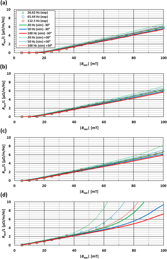
Figure 12. Comparison of the calculated dynamic resistance and experimental results for IDC/Ic = (a) 0.3, (b) 0.5, (c) 0.7 and (d) 0.9 for external AC magnetic field amplitudes up to 100 mT (in 5 mT increments) applied at an angle of θ = ±30°. The results are calculated for frequencies of 20, 50 and 100 Hz and the experiments correspond to frequencies of 26.62, 65.44 and 112.5 Hz.
Download figure:
Standard image High-resolution image
Figure 13. Comparison of the calculated dynamic resistance and experimental results for IDC/Ic = (a) 0.3, (b) 0.5, (c) 0.7 and (d) 0.9 for external AC magnetic field amplitudes up to 100 mT (in 5 mT increments) applied at an angle of θ = ±60°. The results are calculated for frequencies of 20, 50 and 100 Hz and the experiments correspond to frequencies of 26.62, 65.44 and 112.5 Hz.
Download figure:
Standard image High-resolution imageThe results clearly show the influence of the asymmetric angular dependence of Jc and n on the dynamic resistance. Figures 12 and 13 show that positive (dotted lines) and negative (solid lines) field angles result in different slopes of Rdyn in the linear regime and a different onset of 'lift-off' behaviour (for I = 0.9Ic). These asymmetric effects are caused by the different values of Jc and n at +∣θ∣ and −∣θ∣ respectively. For example, and referring back to figure 2, the Jc of the wire at θ = +30° (and θ = +210° for the negative half-cycle of the applied field) is comparatively lower than at θ = −30° (i.e., at θ = +150° and +330° in figure 2). Hence, the slope of Rdyn is higher for θ = +30°, and the 'lift-off' criteria is satisfied at a lower value of ∣Bapp∣. The same is true for the ±60° results shown in figure 12.
In summary, the dynamic resistance in an HTS coated-conductor wire can be mostly determined by the perpendicular field component with subtle differences determined by the angular dependence of the superconducting properties of the wire, which can be included in detail within the numerical modelling framework.
2.3. Dynamic resistance for parallel applied magnetic fields: θ = ±90°
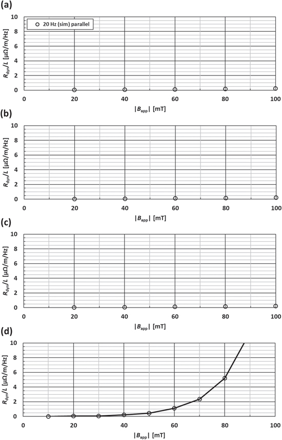
Finally, in this section, the dynamic resistance in parallel applied magnetic fields (at an angle θ = ±90°) is simulated using the same numerical framework. Figure 14 shows the calculated dynamic resistance for IDC/Ic = (a) 0.3, (b) 0.5, (c) 0.7 and (d) 0.9 for parallel magnetic fields up to 100 mT (in 20 mT increments for (a)–(c) and 10 mT increments for (d), and f = 20 Hz). There is negligible dynamic resistance generated until the total driven transport current exceeds Ic of the wire (in this case, when IDC/Ic = 0.9 and ∣Bapp∣ is about 40 mT or higher), resulting in the 'lift-off' regime explained earlier. This provides further evidence that the dynamic resistance in an HTS coated-conductor wire is determined mostly by the perpendicular component of the applied magnetic field and agrees with experimental measurements presented in [31]. This is in direct contrast with BSCCO wires [4, 44]. From the viewpoint of practical applications, it is therefore the perpendicular component of any external, time-varying magnetic field that is of most interest, having a dominant impact on the generated dynamic resistance.
Figure 14. Calculated dynamic resistance for IDC/Ic = (a) 0.3, (b) 0.5, (c) 0.7 and (d) 0.9 for parallel magnetic fields (at an angle θ = ±90°) up to 100 mT (in 20 mT increments for (a)–(c) and 10 mT increments for (d); f = 20 Hz).
Download figure:
Standard image High-resolution image
3. Conclusion
In this paper, a 2D numerical model based on the finite-element method and implementing the H-formulation is used to calculate the dynamic resistance and total AC loss in a coated-conductor HTS wire carrying an arbitrary transport current and exposed to background AC magnetic fields up to 100 mT. The measured angular dependence of the superconducting properties of wire are used as input data, and the model is validated using measured experimental data for magnetic fields perpendicular to the plane of the wire, as well as at angles of θ = 30° and 60°.
The model provides important insights into the origin and characteristic behaviour of dynamic resistance, including its relationship with the applied current and field, the wire's superconducting properties, the threshold field and the onset of nonlinear flux-flow resistance. The key conclusions of the paper can be summarised as follows.
- (1)The normalised total AC loss of the superconducting wire (which includes contributions from both the magnetisation loss, Qmag, and the dynamic resistance, Qdyn) exhibits particular maxima and minima turning points. The maxima correspond to the threshold field, Bth, above which there is no longer a shielded region inside the wire and dynamic resistance occurs, and these maxima shift to lower values of applied field with increasing IDC. The minima observed at higher transport currents relates to the emergence of an additional nonlinear flux-flow resistance term that arises once the total driven transport current exceeds the field-dependent Ic of the wire.
- (2)The dynamic resistance is calculated from the average electric field across the entire conductor cross-section. The time-dependent waveform of this average electric field shows that dynamic resistance is incurred when d∣Ba(t)∣/dt is largest, i.e., in the region around Ba(t) = 0. In contrast, the generation of the flux-flow resistance manifests itself as a spike in the voltage when d∣Ba(t)∣/dt is lowest, i.e., at the maxima and minima of the applied field, ±Bmax. Additionally, there is some noticeable asymmetry of the voltage between half-cycles related to the angular dependence of the superconducting properties of the wire.
- (3)Calculated values of the dynamic resistance as a function of applied field angle show that the dynamic resistance can be mostly determined by the perpendicular field component. However, our calculations indicate subtle angular asymmetries that have not previously been experimentally reported. These are determined by the angular dependence of the superconducting properties of the wire. We also observe that the dynamic resistance under parallel applied fields is essentially negligible until Jc is exceeded and flux-flow resistance occurs.
This numerical modelling framework provides a useful and flexible tool to predict the characteristics of dynamic resistance generated in any HTS coated-conductor wire for which the relevant geometric and superconducting properties are known, as well as the possibility of assessing the emergence and impact of dynamic resistance in more complicated arrangements of conductors, such as multiple-wire stacks, cables and coils.
Acknowledgments
The authors kindly thank Dr Stuart Wimbush, Robinson Research Institute, Victoria University of Wellington, for the Ic(B, θ) and n(B, θ) measurements of the wire. Mark Ainslie would like to acknowledge financial support from an Engineering and Physical Sciences Research Council (EPSRC) Early Career Fellowship EP/P020313/1. Additional data related to this publication are available at the University of Cambridge data repository (https://doi.org/10.17863/CAM.20647). This work was also supported in part by the Japan Society for the Promotion of Science (JSPS).