
Abstract
When a type II superconductor carrying a direct current is subjected to a perpendicular oscillating magnetic field, a direct current (DC) voltage will appear. This voltage can either result from dynamic resistance effect or from flux flow effect, or both. The temperature variation in the superconductor plays an important role in the nature of the voltage, and there has been little study of this so far. This paper presents and experimentally verifies a 2D temperature-dependent multilayer model of the second generation (2G) high temperature superconducting (HTS) coated conductors (CC), which is based on H-formulation and a general heat transfer equation. The model has coupled the electromagnetic and thermal physics, and it can simulate the behavior of 2G HTS coated conductors in various working conditions where the temperature rise has a significant impact. Representative electromagnetic phenomena such as the dynamic resistance effect and the flux flow effect, and thermal behavior like quench and recovery have been simulated. This thermal-coupled model is a powerful tool to study the thermal-electromagnetic behaviors of 2G HTS coated conductors in different working conditions, especially when the impact of temperature rise is important. This multilayer model is also very useful in analyzing the impact of different layers in the 2G HTS CCs, especially the metal stabilizer layers. It has been proven to be a very powerful tool to help understand more complicated characteristics in the CCs which could not be accurately measured or simulated by previous numerical models. The work is indicative and very useful in designing ac magnetic field controlled persistent current switches and flux pumps, in terms of increasing the off-state resistance, analyzing different sources of losses, minimizing detrimental losses, and enhancing the safety and stability.
Export citation and abstract BibTeX RIS

Original content from this work may be used under the terms of the Creative Commons Attribution 4.0 licence. Any further distribution of this work must maintain attribution to the author(s) and the title of the work, journal citation and DOI.
1. Introduction
When an external AC magnetic field is applied perpendicular to a direct current carrying HTS coated conductor, a net flux motion will be triggered. Some magnetic flux enters the superconductor from one side, traverses across the central region where DC current flows, and leaves the conductor from the other side of the conductor. A DC electric field in the same direction of transport current appears and a DC voltage along the superconductor is induced. This phenomenon is known as the 'dynamic resistance effect' [1–5]. A similar phenomenon can be observed in a direct current carrying HTS tape when vibrating with a high frequency in a DC applied field [6]. The DC voltage arises from the interaction between the transport DC current and moving magnetic fluxons within the superconductor, which is a modulation of the vortex spatial distribution [4]. Dynamic resistance is very useful and is utilized as a key mechanism in persistent current switches [7–10] and HTS flux pumps [11–22]. It is also very common for a DC carrying coated conductor to work in an external AC magnetic field, such as in HTS motors and generators [23–26], levitation [27, 28], and HTS power cables [29–31].
Dynamic resistance incurs a dissipative loss effect and generates heating power in the superconductor. When carrying large transport current and working in high background field, heat will accumulate in the CC. The superconductivity of the HTS CC are sensitive to the temperature variation [32]. The temperature rise will impact on the electromagnetic behaviors of the CC significantly. The HTS coated conductor may even be damaged by a temperature increase during a local quench [32]. There has been much previous research on dynamic resistance. A theoretical analysis on the dynamic resistance effect has been done by Oomen et al [2]. Numerous solid experimental investigations into dynamic resistance had been presented by Uksusman et al [4] and Jiang et al [5]. Numerical models for the dynamic resistance have also been built by Ainslie et al [33] and Li et al [34]. A dynamic-resistance-incurred flux pump model was also proposed by Geng and Coombs [35]. However, previous numerical models [33–35] for the dynamic resistance have not considered the impact of the temperature rise, which is of great importance to the performance, safety, and stability of the HTS applications.
Moreover, in previous numerical models [33–35] for the dynamic resistance, the multilayer structure of 2G HTS CC has been oversimplified into a single layer structure, where the impact of each layer and the interaction between different layers in the real 2G HTS CC cannot be simulated. It hinders our further understanding and in-depth investigation into the complicated characteristics inside the HTS CCs, such current sharing among different layers of the CCs, and different loss components in different layers of the CCs. These characteristics are also vital to the design of HTS applications.
In this paper, we build a 2D thermal-coupled multilayer model for the HTS CC based on the H-formulation [36] and a heat transfer equation [37–40]. It has successfully resolved the above two major problems. Both temperature dependency and field dependency have been considered in this model. Our results show that the thermal-coupled model can correctly simulate the electro-thermal response of the DC carrying CC conductor to the external applied field with various magnitudes. Dynamic resistance effect, flux flow effect, quench and recovery phenomena can be successfully simulated. This multilayer model is very close to the real structure of the 2G HTS CCs, making it very useful in analyzing the impact of different layers in the 2G HTS CCs, especially the metal stabilizer layers. It has been proven to be a very powerful tool to help understand more complicated characteristics inside the CCs which could not be accurately measured or simulated by present numerical models [33–35] for the dynamic resistance, such as the temperature distribution, current sharing among different layers of the CCs, and different loss components in different layers of the CCs.
This paper presents the modelling techniques and our experimental verification for this model. The powerful analytical functions of this model are presented and explained in detail. By using this model, we incidentally discovered and successfully verified the shielding effect and the current sharing ability of the Cu-stabilizer. The impact of the Cu-stabilizer incurred by these multiple effects has been analysed, including on dynamic resistance, dynamic voltage, losses, and the risk of quench of the HTS CC. The work is indicative in designing ac magnetic field controlled persistent current switches [7–10] and flux pumps [11–22], in terms of increasing the off-state resistance, analyzing different sources of losses, minimizing detrimental losses, and enhancing safety and stability.
2. Modelling methodology and experimental setup
2.1. Model description
As shown in figure 1, the 2G HTS CC has a multilayer structure, including a high temperature superconducting ReBCO layer (1 μm), a substrate (Hastelloy) layer (50 μm), a buffer stack layer (≈0.2 μm), two silver overlayers (≈2 μm), two copper (Cu) stabilizer layers (20 μm). Figure 2 shows the schematic drawing of the 2D temperature-dependent multilayer model for simulating the thermal-electromagnetic behaviors of a 2G HTS coated conductor when carrying a direct current and subjected to an AC perpendicular magnetic field. In this model, the multilayer 2G HTS CC is simplified into a four-layer model, which contains a YBCO (superconducting) layer (1 μm), a substrate layer (50 μm), and two copper (Cu) stabilizer layers (20 μm) on both sides of the tape. The silver overlayers and the buffer stack layer are neglected since they are too thin compared to the substrate layer and copper stabilizer layers. The width of the CC is 6 mm. This multilayer model is very close to the real structure of the 2G HTS CCs, making it very useful in analyzing the impact of different layers in the 2G HTS CCs, especially the metal stabilizer layers. It will be proved to be a very powerful tool to help understand more complicated characteristics inside the CCs which could not be accurately measured or simulated by previous numerical models [33–35], such as the temperature distribution, current sharing among different layers of the CCs, and different loss components in different layers of the CCs.

Figure 1. Diagram of coated conductor structure and layer composition. Reproduced with permission from [41].
Download figure:
Standard image High-resolution image
Figure 2. Schematic drawing of the 2D temperature-dependent multilayer model for a direct current carrying HTS coated conductor wire under perpendicular AC magnetic fields. (a) is the electromagnetic module, which is responsible for calculating electromagnetic variables including the heating power (q) in each element; (b) is the thermal module for calculating the temperature (T) of each element. The Bapp is the instantaneous external AC magnetic field perpendicular to the HTS tape surface. It is the DC transport current flowing along the HTS coated conductor tape.
Download figure:
Standard image High-resolution imageThe model consists of two mutually coupled modules: an electromagnetic module and a thermal module. They are mutually coupled through the calculated heating power (q) and the temperature dependence of critical current density Jc(B,T) of the superconductor. In each calculation step, the electromagnetic module calculates the heating power (q) in each element; at the same time, the thermal module calculates the temperature (T) of each element based on the heating power (q) from the electromagnetic module. The temperature dependent critical current density Jc(B,T) of each element in the electromagnetic module is simultaneously updated according to the temperature (T) results calculated by the thermal module in each step. The model is built and solved by commercial finite element software COMSOL Multiphysics.
It is worth mentioning that: this model is also extensible and multifunctional for simulating a variety of different working conditions, such as (i) transporting an AC or DC or zero current, (ii) subjecting to an AC, DC, or zero perpendicular magnetic field; (iii) subjecting to an external magnetic field at an arbitrary angle by rotating the HTS CC wire in the X–Y plane. In the future, this model can be used in many other interesting investigations for 2G HTS CC wires.
2.2. Electromagnetic module
2.2.1. Governing equations
The governing equations for the electromagnetic module are derived from Faraday's law and Ampere's law:

where μ0 is the permeability of free space, μr is the relative permeability. For the superconducting layer and non-magnetic layers, the relative permeability is μr = 1. The equations are solved by using the H-formulation [36]. In 2D geometry, H = [Hx, Hy], which represents the components of magnetic field in the x and y directions. The induced electric field and the current density are perpendicular to the cross section and are defined as Ez and Jz. By substituting H =[Hx, Hy], E = Ez and J = Jz into equation (1), we obtain:
The resistivity (ρ) of the superconducting element in YBCO layer follows the E–J power law [42, 43]:

where E0 = 10−4 V m−1, n = 21 [36–38], and Jc(B, T) is the temperature and magnetic field dependent critical current density, which will be explained in section 2.2.2. The resistivities (ρ) for the non-superconducting elements are set as constant values. The resistivity (ρ) is 8 × 10⁻⁹ Ωm for Cu-stabilizer layer, 1 × 10⁻⁶ Ωm for substrate layer, and 100 Ωm for air region.
2.2.2. Magnetic field and temperature dependence
The critical current density of the 2G HTS coated conductor is sensitive to and influenced by the variation of both the temperature and the magnetic field density. The magnetic field and temperature dependent critical current density are given as:

where Jc0 is the self-field critical current density at 77 K, Jc(B) represents the coefficient of magnetic field dependence, and Jc(T) represents the coefficient of temperature dependence. Jc(B) ∈ [0, 1], and Jc(T) ∈ [0, 1]. The self-field critical current is set as 140 A, according to the experimental measured self-field critical current from a 2G HTS CC wire manufactured by SuperPower [7]. Jc0 is set as 2.33 × 10¹⁰ A m−2, which is calculated according to self-field critical current (140 A) and the cross-section area of the YBCO layer (6 mm wide × 1 μm thick).
Jc(B) is calculated through an anisotropic model [44–46], which is given as:

where Bpara and Bperp represent the flux density parallel and perpendicular to the wide tape surface, respectively. k, Bc and b are three parameters controlling the Jc(B) curve. These three parameters are obtained by curve fitting on experimental measured critical current data for a specific 2G HTS CC wire from the HTS CC manufacturers. In our model, we use the values for k, Bc and b from a SuperPower coated conductor wire in [45]: Bc = 0.3 T, k = 0.25 and b = 0.6. In the experimental verification (section 2.4), a SuperPower SCS4050 2G HTS coated conductor is used, which is the same 2G HTS coated conductor wire with the one used in [45].
Jc(T) is calculated according to equation (6), which has been adopted in [37, 38]
where T is the temperature for each element in the superconducting (YBCO) layer, which is calculated through the thermal module. T0 = 77 K is the starting temperature of the 2G HTS CC in the model, which is the same with the temperature of the surrounding liquid nitrogen, Tc = 92 K is the critical temperature, above which the HTS element totally losses its superconductivity.
2.2.3. Boundary conditions
For the real multilayer 2G HTS coated conductor wire, a portion of transport current will flow into protective metal layers such as Cu-stabilizer layers under certain conditions. These conditions include when the YBCO layer enters a resistive stage due to the 'dynamic resistance effect', due to a large overcurrent exceeding the YBCO critical current, due to a temperature rise of the YBCO layer, or due to high external DC or AC field. Our four-layer model can simulate the current sharing among different layers of the CC, which will help further our understanding about the interaction between different layers in the 2G HTS CC. The transport current (It) is set as the sum of the current in each layer:
where, s refers to the cross-section area of each layer. IYBCO, ICu_upper, ICu_lower and ISub is the DC transport current in the YBCO layer, the upper Cu-stabilizer layer, the lower Cu-stabilizer layer, and the substrate layers respectively. JYBCO JCu_upper, JCu_lower, and JSub are the current density in each element of above four layers. The transport current It is applied to the CC through a 'Pointwise Constraint' in COMSOL. To avoid non-convergence in the model calculation, it takes 0.01 s for the transport current to ramp linearly from zero to the preset constant value.
The applied ac perpendicular magnetic field (Bapp) is generated by a pair of electro-magnets with a narrow flux gap (≈1 mm). Each magnet consists of a pair of windings and an iron core, which is similar to that described in [35]. A series of sinusoidal magnetic waveform (Bapp) with different peak magnitudes and frequencies are applied perpendicular to the surface of the HTS CC tape in the model. The boundary of the air region is far away from the superconductor, therefore the perpendicular component of magnetic field to the boundary is very small and can be set as zero in the model.
2.2.4. Loss, voltage, and resistance
The loss (q) per length meter (W m−3) generated in each element of the CC is the heating power source for each element in the thermal module. It is also a key parameter linking electromagnetic module and thermal module. q is calculated by equation (8):

In the multilayer 2G HTS coated conductor wire, different layers produce different types of loss: the superconducting (YBCO) layer generates a transportation loss and a magnetization loss. The transportation loss origins from the dynamic resistance and flux flow resistance. The magnetization loss normally refers to hysteresis loss during the magnetization process of the superconductor (YBCO). Meanwhile, metal layers such as Cu-stabilizer will incur a transportation loss due to the metal's (copper's) resistivity if carrying a transport current, and an eddy current loss if subjected to a perpendicular AC magnetic field (Bapp). The existence of the eddy current in the Cu-stabilizer has a significant impact on the behavior of the direct current carrying HTS CC when subjected to a perpendicular AC magnetic field. It will be analyzed in detail in the sections 3.3 and 3.4. To sum up, the loss of the HTS CC contains three types of loss, including transportation loss, magnetization loss, and eddy current loss.
Total loss of each layer per length meter (Qlayer) (W m−1) can be calculated by a surface integral, as shown in equation (9), where s refers to the cross-section area of each layer. The total loss of the CC (Qcc) can be obtained from the sum of loss in four layers. Since the resistivity of substrate layer is much larger than Cu-stabilizer layer, current in substrate (ISub) layer is negligible. QSub is also very small and negligible. In order to distinguish the transport loss from magnetization loss or the eddy current loss, the voltage per length-meter (Vcc/L) (V m−1) of the CC along the tape length direction should be calculated first. It is the average electric field density along the length direction of the CC wire, which can be calculated by equation (10). sYBCO refers to the cross-section area of YBCO layer. The transportation loss (Qtrans) in a certain layer can be calculated by equation (11), where Itransport refers to the transport current in the same layer, for example IYBCO in YBCO layer, ICu_upper and ICu_lower in upper and lower Cu-stabilizer layer in figure 3. Afterwards, as shown in equation (12), the magnetization loss (Qmag) in YBCO layer can be calculated by removing out the transportation loss (Qtrans) from the total loss of YBCO layer (QYBCO) which can be calculated through equation (9). Similarly, as shown in equation (13), the eddy current loss (Qeddy) in the Cu-stabilizer layer can be calculated by removing the transportation loss (Qtrans) from the total loss of Cu-stabilizer layer (QCu) which can be calculated through equation (9)


Figure 3. The equivalent circuit of the multilayer HTS CC wire.
Download figure:
Standard image High-resolution imageThe resistance per length-meter (RYBCO/L) (Ω m−1) of YBCO layer along the tape length direction can be calculated by equation (14). The waveform of the RYBCO/L is an important parameter to determine the status of the YBCO layer, such as a simple status only containing a dynamic resistance, or a mixed status containing both the dynamic resistance effect and flux flow effect. The total resistance of the HTS CC is mainly determined by the parallel resistances, mainly the YBCO layer and two Cu-stabilizer layers. The impact of the high resistivity substrate layer is very small and can be ignored. The equivalent circuit is presented in figure 3, from which we know that Vcc/L = Vybco/L = Vcu/L.
2.3. Thermal module
2.3.1. Governing equation
The thermal module calculates the temperature for each element in the coated conductor. In each calculation step, it is responsible for updating the temperature of the CC wire, which is important for updating the coefficient of temperature dependence Jc(T) as shown in equations (4) and (6). The thermal module is based on the general heat transfer equation (15):

where d is the mass density (kg m−3), C is the heat capacity (J kg−1K−1)), k is the thermal conductivity (W m−1K−1). The mass density for YBCO layer is 5900 kg m−3, it is 8000 kg m−3 for Cu-stabilizer, and 8280 kg m−3 for substrate. The heat capacity C and thermal conductivity k of the YBCO, substrate, and copper (Cu-stabilizer) in this model are temperature dependent, which are presented in figure 4. The data for C and k are obtained from reference [47–50]. q (W m−2) is the heating power source in each element, which is calculated by equation (8) in the electromagnetic module. This general heat transfer equation (15) means that the temperature variation is a final result from two impacting factors: the heating power (q) generated inside the element, and the heat transfer between the element itself and the surrounding elements.

Figure 4. Thermal conductivity (k) and heat capacity (C) of the YBCO, Cu-stabilizer, and substrate.
Download figure:
Standard image High-resolution image2.3.2. Heat transfer boundary condition
An accurate setting for heat transfer boundary condition is critical for the accuracy of the thermal-coupled model. It significantly influences the thermal-electromagnetic behavior of the 2G HTS CC in the simulation model. In our model, a convective heat flux type boundary condition is adopted, which is highlighted by red line in figure 2(b). The convective heat flux boundary condition can be expressed as:

where Q is the heat transfer (W m−2) between the liquid nitrogen and the surface of the HTS CC tape, Text is the temperature of liquid nitrogen surrounding the coated conductor, and h is the heat transfer coefficient (W m−2 K−1) representing the cooling (heat transfer) capability of the liquid nitrogen by liquid-to-solid surface contact. Text is set as a constant value at 77 K. h value is an important parameter in heat transfer boundary condition. In reference [37], the h is set as 10 000 W m−2 K−1. But in our verification experiment, the CC tape is placed in a narrow gap of the magnet, so the cooling condition is not as good as in an open space in the liquid nitrogen. When the heating power is large, bubbles will be generated in the liquid nitrogen, which is very detrimental to the heat dissipation of the CC tape in the narrow gap. So, h value should be lower in this model. We have tried different values for h between 500 to 10 000, but finally got reasonable simulation results when h = 800 W m−2 K−1. Table 1 gives a brief summary of the specifications of the HTS coated conductor model.
Table 1. Specifications of the HTS coated conductor model.
| Parameters | Value |
|---|---|
| Tape width | 6 mm |
| Thickness of superconducting layer | 1 μm |
| Thickness of substrate layer | 50 μm |
| Thickness of stabilizer layer | 20 μm |
| μ0 | 4π × 10−7 H m−1 |
| n (E–J power law index) | 21 |
| Tape self-field Ic0 at 77 K | 140 A |
| Jc0 | 2.33 × 10¹⁰ A m−2 |
| E0 | 10−4 V m−1 |
| Bc | 0.3 T |
| k | 0.25 |
| b | 0.6 |
| T0 | 77 K |
| Tc | 92 K |
| h | 800 W m−2 K−1 |
Table 2. Specifications of the Superpower SCS4050 coated conductor wire.
| Parameters | Value |
|---|---|
| Tape width | 6 mm |
| Superconducting layer thickness | 1 μm |
| Substrate layer thickness | 50 μm |
| Stabilizer layer thickness | 20 μm |
| Tape self-field Ic at 77 K in the magnet gap | 135 A |
2.4. Experimental verification
To validate this model, we experimentally measured the voltage response of a DC carrying 2G HTS CC sample wire when subjecting to a series of perpendicular AC magnetic field with various magnitudes. A 10 cm long and 6 mm wide SuperPower SCS4050 coated conductor is used, which has two 20 μm thick copper stabilizers on both sides. Table 2 presents the specifications of the Superpower SCS4050 coated conductor wire. The self-field critical current is around 135 A (at 77 K, with 10−4 V m−1 criterion) when the coated conductor is placed in the narrow gap (≈1 mm) of the iron core of the electromagnet. The gap of the iron core is very narrow, and the iron core can concentrate the magnetic flux, which increases the self-field of the coated conductor tape when transporting a DC current. The increased self-field will lead to the decrease of the self-field critical current of the CC tape. The original self-field critical current should be slightly higher than 135 A. That is the reason why Ic0 (at 77 K, self-field) in the simulation model is set as 140 A. Our results in figure 10 can verify our explanation about this phenomenon. The tape critical current Ic in narrow gap degrades to around 0.95 Ic0 (around 135 A) when the applied field (Bapp) is removed. The AC field is generated by an electromagnet with a copper winding of 80 turns. The CC is placed in a narrow air gap of the electromagnet. The cross section of the gap is 2 cm × 1.2 cm. The AC field is normal to the CC's wide surface. The voltage response of the CC is measured via a pair of voltage taps soldered to the CC surface with a 2 cm separation. The ac field magnitude is monitored by a pick-up coil winding on the gapped ferrite core. The transport current is supplied by an Agilent 6680A constant current source. The field is magnet is powered by an EP4000 audio amplifier with a wide frequency range. All signals are acquired by an NI-PCIe 6221 DAQ card. More details about the experimental setup can be found in [6].
3. Result and analysis
3.1. Dynamic resistance effect and flux flow effect
Representative electromagnetic phenomena such as dynamic resistance effect and flux flow effect can been well simulated by our model. Figures 5(a1) and (b1) show the electric field response of the CC to a 1 kHz, 50 mT (peak) applied field. Figure 5(a1) is the simulation result and figure 5(b1) is the experimental data for comparison. The chosen field magnitude is relatively low so that the superconductor is not driven to flux flow state at the peak of the applied field. The simulation result for 'dynamic resistance effect' is in good agreement with the experimental data in terms of waveform: there are two peaks in the electric field waveform during each cycle of the applied field. Both peaks appear around the zero-crossing of the applied field, when the field changing rate is the highest. And the electric field is close to zero around the peaks of the applied field, when the field rate of change is the lowest. In terms the magnitude of the electric field waveform, there is still a slight difference between the simulation and experiments. The difference is acceptable and could be caused by many factors: the adoption of a Jc(B) formula (equation (5)) in instead of experimental measured data, the simplified temperature dependence Jc(T) formula (equation (6)), and the neglect of silver overlayers and the buffer stack layer, and so on.

Figure 5. Electrical field generated on the CC in simulation (a1), (a2) and experiment (b1), (b2) when: field magnitude (peak) is around 50 mT (a1), (b1), 200 mT (a2), (b2), and 400 mT (a2), (b2).
Download figure:
Standard image High-resolution imageFigures 5(a2) and (b2) show the result when the applied field magnitude is increased to around 200 mT and 400 mT, respectively. The waveforms are very different from the previous ones when the applied field is low. The first difference is that the electric field does not go back to zero at the peaks of the applied magnetic field, so that the electric field value is always over zero, and the curve seems to be 'floating'. The second difference is that there are more than two peaks in the electric field during each cycle of the applied magnetic field. There are 'side peaks' in the electric field appearing at the peaks of the applied field. Comparing the 200 mT result and the 400 mT result, we can clearly see that the 'side peak' values increases with the applied field. These two significant differences can be explained by the 'flux flow effect': due to the strong dependence of critical current density to the perpendicular applied field, the tape is intermittently driven into flux flow region when the instantaneous value of the applied field is high, especially around its peaks. When the applied field magnitude is increased to 200 mT and 400 mT, we can observe both the 'dynamic resistance effect' and 'flux flow effect'. Therefore, we can see multi-peaks in the electric field waveform both at the applied field zero-crossings time-point as well as at its peaks time-point.
Both the waveforms under low applied field and high applied fields are in good agreement with the previous theoretical analysis [2], test results [4, 5], and simulation results [33, 34].
3.2. Quench and recovery
This temperature dependent multilayer model is a very powerful tool to help us better understand complicated characteristics in the HTS CCs. which could not be accurately measured, such as the temperature distribution, current sharing between multi layers, the resistance of the superconducting layer, instant critical current variation, and different loss components in different layers of the CCs.
3.2.1. Voltage response
In either the previous dynamic resistance model or flux flow model, the temperature rise in the superconductor is not considered. This is not valid when the applied field is with high frequency, high magnitude, and long duration. In this case, quench behavior may happen in the CC. By using our temperature-dependent model, the thermal-electromagnetic behaviors of 2G HTS coated conductors can be successfully simulated. Figure 6 shows the electric field response of the CC to 20 cycles of 1 kHz applied field. Our experimental results show that the impact of the temperature rise is not obvious when the field frequency is low. So, we focus on the high frequency range around 1 kHz here. Figures 6(a1)–(a3) are the simulation results when the applied field (peak) is 50 mT, 200 mT and 400 mT. Figures 6(b1)–(b3) are the experimental data for comparison. The transport current is set as 80 A (around 0.6 Ic0) in both simulation and experiment. The simulation results are in well accordance with the experimental data, especially in terms of waveform shape and recovery time. The difference in magnitude between the simulation and experiments is acceptable.

Figure 6. The electric field response of the CC to 20 cycles of 1 kHz applied field when the applied field (peak) is 50, 200, and 400 mT. (a1), (a2) and (a3) are simulation results, (b1), (b2), and (b3) are the experimental data for comparison.
Download figure:
Standard image High-resolution imageWhen the field magnitude is relatively low, the electric field response of the CC is stable. And it recovers to zero immediately when the applied field is removed. When the applied field magnitude is increased to 200 mT, the electrical field peak value increases gradually with time, which is different from the case when the applied field is low. At the same time, the valley value gradually increases and does not return to zero ('floating') after a time period. Both are different phenomena as well. But the electric field still can recover to zero quickly when the field is removed. When the applied field increases to 400 mT, the electrical field is both increasing and 'floating' at the same time. When the field is removed, an obvious 90 ms time-delay of electrical field returning to zero is observed, which is regarded as thermal quench and recovery behavior. Both our numerical and experimental results show that the CC becomes unstable and even quenches when a magnetic field with high frequency, high magnitude, and long duration is applied. By comparing the simulation and experimental waveforms, our thermal-coupled model has been successfully validated to be capable of correctly simulating the electro-thermal response of the DC carrying CC conductor to the external applied field with various magnitudes.
3.2.2. Temperature variation
Monitoring the temperature variation of the 2G HTS CC wire is another important function of this temperature-dependent model. Figure 7(a) shows the temperature rise of the CC when 20 cycles of 1 kHz applied field are applied. When the field magnitude is relatively low (50 mT), the temperature of the CC rises slightly, from 77 to 78 K. When the field is 200 mT, the temperature rise is moderate (6 K, from 77 to 83 K). But when the field increases to 400 mT, the temperature rise is considerable (12 K, from 77 to 89 K), and it decreases slowly after the field is removed. The high temperature rise and very slow cooling speed lead to the fast increase of the electrical field (Vcc/L) and the long recovery time (90 ms) of the HTS CC as shown in figures 6(a3) and (b3).

Figure 7. (a) The average temperature of coated conductor, and (b1)–(b3) the coefficient of temperature dependence Jc(T) distribution along the length direction in the YBCO layer at different instants of time when the field magnitude is 50, 200, and 400 mT.
Download figure:
Standard image High-resolution imageFigures 7(b1)–(b3) show the coefficient of temperature dependence Jc(T) distribution along the length direction in the YBCO layer at different instants of time when the field magnitude is 50, 200, and 400 mT. Results show that the degradation of Jc(T) is more severe at two edges of the CC wire. It is caused by the faster and higher temperature rise at two edges of the CC wire than the temperature rise in the center. This is because the current density on the two ends is higher, then the electrical field is higher, and therefore the loss in two ends is larger. Our results indicate that the most vulnerable part of the HTS CC wire is at the two edges when carrying a DC transport current and subjected to a perpendicular AC field. This finding is very indicative for the design of HTS current switches and switches-based flux pump. Our model is also very useful in analyzing the quench and recovery process of HTS CC switches.
3.2.3. Current distribution
This multilayer structured model is very powerful to help study the current sharing and different loss components in different layers, which could not be accurately measured. Figure 8 shows the current distribution of the CC in YBCO layer and one Cu-stabilizer layer. We have verified that the current in the upper and lower Cu-stabilizer layers are exactly the same, so here only the current in one Cu-stabilizer (upper or lower) layer is plotted. When the field magnitude is relatively low (50 mT), the transport current of the CC mainly flows in the YBCO layer and a very small proportion flows into Cu-stabilizer. When the field increases to 200 mT, a larger proportion of transport current enters Cu-stabilizer. When the field increases to 400 mT, a great proportion of the transport current flows into the Cu-stabilizer. Moreover, when the temperature of the CC increases, more and more current enters Cu-stabilizer due to the temperature dependency of the critical current density of the YBCO layer. When the 400 mT field is removed, a long recovery time is needed for the transport current in Cu-stabilizer to return to YBCO layer, which is a typical characteristic of the thermal quench and recovery behavior.

Figure 8. Current distribution in YBCO and the upper (or lower) Cu-stabilizer layer. We have verified that the current in upper and lower Cu-stabilizer layers are totally the same, so here only the current in one Cu-stabilizer (upper or lower) layer is plotted.
Download figure:
Standard image High-resolution image3.2.4. Resistance of superconducting layer
Figure 9 shows the resistance of YBCO layer and Cu-stabilizer. When the field magnitude is relatively low (50 mT), the resistance of the YBCO layer is very small and is solely due to dynamic resistance. When the field increases to 200 mT, the resistance of the YBCO layer increases to a higher level. When the field magnitude rises to 400 mT, the resistance of YBCO layer is comparable to the constant resistance of Cu-stabilizer layer and the instantaneous value finally surpasses the resistance of Cu-stabilizer due to the temperature rise. The waveform shows that the resistance of YBCO layer consists of both dynamic resistance and flux flow resistance. When the 400 mT field is removed, the resistance of the YBCO layer does not recover to zero immediately because the YBCO layer is still in flux flow region. The resistance variation of the YBCO layer compared to the constant resistance of Cu-stabilizer in figure 9 can explain the current distribution between YBCO layer and Cu-stabilizer in figure 8. Since the total resistance of the HTS CC is determined by the parallel resistances, mainly the YBCO layer and two Cu-stabilizer layers, the variation of the resistance of YBCO layer will result in the change of the total resistance of HTS CC.

Figure 9. Resistance (Ω m−1) of YBCO layer and Cu-stabilizer layer.
Download figure:
Standard image High-resolution image3.2.5. Critical current
Figure 10 shows the critical current response of the YBCO layer to the applied field. The critical current waveform can help determine the working condition of the 2G HTS CC wire. When the field magnitude is relatively low (50 mT), the degradation in critical current of the YBCO layer is very slight. When the field magnitude increases to 200 and 400 mT, the critical current decreases greatly to different extent, which results in the current sharing in figures 7(b) and (c). When the 400 mT field is removed, the critical current of the YBCO layer is still much lower than transport current, so consequently the current flows through the Cu layer. During the recovery process, the critical current gradually increases, surpasses the transport current, and finally recovers to its initial state.

Figure 10. Critical current (Ic) response of YBCO layer to the applied field (Bapp).
Download figure:
Standard image High-resolution image3.3. Loss analysis
In the applications of dynamic resistance such as persistent current switches [7–10] and flux pumps [11–22], losses are a very important issue. It would be desirable to know the sources of the losses and to minimize them. Compared to previous model, our multilayer thermal coupled model can help calculate the different loss components from different layers. It can also help understand the loss variation when the temperature rises.
Figure 11 shows the total loss, transport loss, magnetization and eddy loss of the CC when a perpendicular AC magnetic field is applied. The eddy loss is induced in the Cu-stabilizer layer. When the field magnitude increases, the total loss increases. When the field magnitude is relatively large (400 mT), the total loss decreases with time, among which the total amount of the magnetization loss and eddy loss drops while the transport loss increases.

Figure 11. The total loss, transport loss, and the total amount of magnetization loss and eddy loss of the CC when a perpendicular AC magnetic field is applied.
Download figure:
Standard image High-resolution imageMoreover, the if the impact of temperature rise is not considered, the ratio of transport loss to total loss drops when the field magnitude increases: the Qcc_trans = 0.238 Qcc (Bapp = 50 mT), Qcc_trans = 0.157 Qcc (Bapp = 200 mT), and Qcc_trans = 0.124 Qcc (Bapp = 400 mT). This phenomenon does not agree well with the traditional theory. According to the traditional theory: critical state model proposed by Bean [51], the ratio of transport loss to total loss should rise and the ratio of magnetization loss to total loss should decrease when the transport current (It) rises closer to critical current (Ic), because more space in the superconducting layer is occupied by the transport current and therefore the magnetization loss is less.
In order to understand the above phenomenon, we further investigate the losses in different layers of the CC, mainly YBCO layer and two Cu-stabilizer layers because losses are mainly generated these two layers. Figure 12 shows the transport loss and magnetization loss of YBCO layer, as well as the transport loss and eddy loss of Cu-stabilizer. The ratio of loss in YBCO layer to the total loss in the whole CC varies greatly when the field magnitude increases. When the field is relatively small (50 mT), the loss of the CC mainly comes from YBCO layer, including magnetization loss and transport loss. When the applied field magnitude increases to 200 mT and 400 mT, the loss generated in Cu-stabilizer increases and eventually becomes the dominant component.

Figure 12. The transport loss and magnetization loss of YBCO layer and Cu-stabilizer.
Download figure:
Standard image High-resolution imageFigure 12 also shows that the magnetization and transportation losses change greatly when the temperature rises, while the eddy current loss in the Cu-stabilizer layer is not affected by temperature. When the field magnitude is 400 mT, the magnetization loss in YBCO layer decreases quickly as the temperature of the CC rises. It results from the decrease of the current carrying ability of YBCO layer. The transport loss in Cu-stabilizer increases greatly because the current is entering the stabilizer layer as the temperature rises. The eddy current is induced by the perpendicular applied AC field, and the resistivity of the copper does not change much during a small temperature rise. So, the eddy current loss in the Cu-stabilizer layer is not affected by temperature.
From the results above, we found that the Cu-stabilizer impacts significantly on the total loss of the CC. The transport loss of Cu-stabilizer is an unavoidable by-product of its helpful current sharing ability. The existence of large eddy loss in the Cu-stabilizer indicate that Cu-stabilizer layer has a shielding effect of the AC external magnetic field. The shielding effect will impact on the dynamic resistance of the YBCO layer, which is worth being studied more carefully. The next section presents our study on the shielding effect of the Cu-stabilizer.
3.4. Impact of Cu-stabilizer layer
3.4.1. Shielding effect and current sharing ability
This section investigates the shielding effect of the Cu-stabilizer layer. In order to better understand the impact of the Cu-stabilizer layer, it's better to separate the impact of the current sharing ability and field shield effect. In order to achieve this goal, a new set of comparison models are designed and simulated: (i) An HTS tape which only contains the YBCO layer and substrate layer, whose upper and lower Cu-stabilizer layers have been removed. (ii) An HTS CC tape which contains both upper and lower Cu-stabilizer layers, but the transport current (It) has been constrained to flowing in the YBCO (Superconducting) layer. In this case, the current sharing ability of the Cu-stabilizer has been removed. (iii) An HTS CC tape which contains both up and down Cu-stabilizer layers and the transport current (It) constraint has been cancelled, so It can be naturally shared by the Cu-stabilizers. It is the same as the model setting in previous sections. Above experiments and simulations have already shown that the temperature rise influences the behaviors of the HTS CC tape significantly. In order to get rid of the influence of the temperature difference between comparison simulations, the heat transfer coefficient h is increased from 800 W m−2 K−1 to 10 000 W m−2 K−1 (a more than 10 times higher level). Our simulation results below will prove that this very high heat transfer coefficient (h) value can help guarantee a same temperature rise for comparison simulation models, which is quite an important precondition for studying the shielding effect of the Cu-stabilizer layer. The peak magnitude of Bapp is 35 mT and the frequency is set as 2 kHz for a more obvious shielding effect. The low frequency range like around 50 Hz has been studied, but the shielding effect is not as significant as in the high frequency range (kHz level). The transport current is still 80 A.
Figure 13(a) shows the temperature curves of three HTS tapes. They are almost the same, which is an important precondition for further analysis and discussion of shielding effect. Figure 13 (b) is the transport current (Iybco) flowing in the YBCO (superconducting) layer in three HTS tapes. Only in tape model (iii), Iybco fluctuates due to the current sharing of Cu-stabilizer layer. Both figures 13(a) and (b) verifies our temperature control and current injection in three comparison models for different HTS tapes.
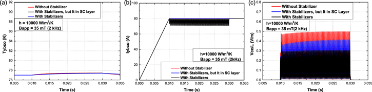
Figure 13. (a) Temperature curves of the YBCO (superconducting) layer in three HTS tapes, (b) transport current (Iybco) flowing in the YBCO layers, and (c) the electrical field (or voltage per meter length) (Vcc/L) generated on three HTS tapes.
Download figure:
Standard image High-resolution imageFigure 13(c) shows the electrical field (or voltage per meter length) (Vcc/L) generated on three HTS tapes. Results show that the existence of Cu-stabilizer layer greatly reduces the electrical field (Vcc/L) generated on DC carrying HTS CC tapes subjecting to AC external applied field (Bapp). It is easy to understand that the current sharing ability of Cu-stabilizer will decrease the electrical field (Vcc/L) because the electrical field or is a product of the resistance (Rybco/L) and current (Iybco) in YBCO (superconducting) layer. However, mechanism is not so simple for the decrease of electrical field (Vcc/L). Our results in figure 14 reveal the existence of the magnetic field shielding effect of the Cu-stabilizer and its impacts on the dynamic resistance of the superconducting (YBCO) layer.
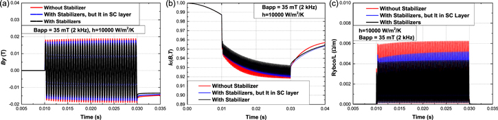
Figure 14. (a) The perpendicular field magnitude (By) at the center point of YBCO layer's up surface of three HTS tapes, (b) the temperature and magnetic field dependent critical current (Ic(B,T)) of three HTS tape, and (c) the resistance (Rybco/L) of superconducting (YBCO) layer of three HTS tapes.
Download figure:
Standard image High-resolution imageFigure 14(a) shows the perpendicular field magnitude (By) at the center point of YBCO layer's up surface, which can tell the intensity of the field shielding effect of Cu-stabilizers. Figure 14(b) shows the temperature and magnetic field dependent critical current (Ic(B,T)) of HTS tape. The temperature curves are the same for three HTS tapes, therefore Ic(B,T) is a good monitor for field shielding effect. Both figures 14(a) and (b) successfully show that the perpendicular field magnitude at the center point of YBCO layer's up surface is reduced due to the upper and lower Cu-stabilizers' shielding effect. Figure 14(c) shows the resistance (Rybco/L) of superconducting (YBCO) layer. Their waveforms show that the resistances are totally dynamic resistance. From [5], we know that the dynamic resistance in a certain fixed width HTS tape is determined by the magnitude of perpendicular component (By) of AC applied external magnetic field, if the field frequency is fixed as well:

So, for tape (ii) (the transport current (It) only flows in the YBCO (Superconducting) layer), the dynamic resistance (Rybco/L) decreases a lot simply because the up and down Cu-stabilizers shield a portion of the perpendicular field (By). For tape (iii), the transport current (It) can be shared by the Cu-stabilizers naturally. This situation is more complicated. Both the current sharing phenomenon and shielding effect of the Cu-stabilizers lead to a further reduced dynamic resistance (Rybco/L). On one hand, the shielding effect of the Cu-stabilizer can reduce the perpendicular field (By) to some extent, which has already been verified in above discussion. On the other hand, when the dynamic resistance appears in the superconducting (YBCO) layer due to the AC perpendicular field, a portion of transport current (It) flows into the upper and lower Cu-stabilizer layers. As a result, Iybco decreases and so the YBCO layer can screen more applied field. The screening effect of the YBCO layer becomes stronger under the same AC field, compared to tape (ii). This also further reduces the AC perpendicular field (By). Figure 14(a) provides good evidence for this explanation, where AC perpendicular field (By) in tape (iii) is further reduced, compared with tape (ii). The further reduced AC perpendicular field (By), caused by both the Cu-stabilizers' shielding effect directly and by their current sharing ability indirectly, finally results in a higher Ic(B,T) and a lower dynamic resistance (Rybco/L) of superconducting (YBCO) layer, which are clearly presented in figures 14(b) and (c) respectively.
Now, let's move back to figure 13(c): the electric field (Vcc/L) generated on three HTS tapes. After the analysis and discussion above, the mechanism behind the decrease of electrical field (Vcc/L) for tape (iii) is clear now: (a) Firstly, Cu-stabilizers' shielding effect directly reduces the dynamic resistance (Rybco/L) of superconducting (YBCO) layer, and the Cu-stabilizers' current sharing ability also indirectly reduces dynamic resistance (Rybco/L) of superconducting (YBCO) layer. (b) Secondly, the Cu-stabilizers share a portion of transport current (It), which reduces the transport current (Iybco) in YBCO (superconducting) layer. As a result, compared to tape (i) and tape (ii), the electrical field (Vcc/L) generated on HTS tape (iii) is further reduced due to the drop in both the resistance (Rybco/L) and transport current (Iybco) in YBCO (superconducting) layer. (For the multilayer coated conductor, Vcc/L = Vybco/L = Vcu_stabilizer/L because the multilayers are electrically connected in parallel).
To conclude, our simulation models and results have deepened our understanding on the impact of the Cu-stabilizer on the behavior of the DC carrying HTS CC tapes subjecting to AC external applied field. The simulation results have verified the shielding effect and current sharing ability of Cu-stabilizer. The existence of the Cu-stabilizers will decrease the dynamic resistance and the dynamic voltage of the HTS coated conductors due to both the shielding effect and current sharing ability, directly and indirectly. Our analysis and discussion here are useful for the future design of HTS persistence current switches, flux pumps, and cables.
3.4.2. Frequency dependence of shielding effect
This section presents the frequency dependence of the shielding effect. Figure 15(a1)–(a3) shows the perpendicular field magnitude (By) at the center point of YBCO layer's up surface under 1, 2, and 4 kHz field frequency, for tape (i) and tape (iii). Figures 15(b1)–(b3) shows the dynamic resistance (Rybco/L) of superconducting (YBCO) layer accordingly. Tape (ii) is not the real situation for the HTS coated conductor, so it is not discussed here. The magnitude of the applied perpendicular AC field is 35 mT, but the measured perpendicular field magnitude (By) at the center point of YBCO layer's up surface is around or less than 20 mT. It is caused by the shielding effect of the whole coated conductor, including the superconducting layer (predominately) and Cu-stabilizer layers (slightly). But it would not influence our study on the frequency dependence of shielding effect below.

Figure 15. The perpendicular field magnitude (By) at the center point of YBCO layer's up surface for tape (i) and tape (iii) under 1 kHz (a1), 2 kHz (a2), and 4 kHz (a3) field frequency. And the dynamic resistance (Rybco/L) of superconducting (YBCO) layer accordingly (b1)–(b3).
Download figure:
Standard image High-resolution imageAs shown in figure 15(a1)–(a3), when the field frequency is 1 kHz, the By decreases slightly due to the existence of Cu-stabilizers. When the frequency increases, the By further decreases due to the existence of Cu-stabilizer. When the field frequency increases to 4 kHz, the field By decreases greatly, by around ¼, due to the existence of Cu-stabilizers. Figure 15(b1)–(b3) shows that the frequency dependency for dynamic resistance (Rybco/L) of superconducting layer is more significant as a result of the existence of Cu-stabilizers. When the field frequency increases to 4 kHz, the dynamic resistance (Rybco/L) of the superconducting layer decreases by around half, as a result of existence of Cu-stabilizers on both sides of the coated conductor.
Figure 16 shows the percentage of the total eddy current loss (two Cu-stabilizer layers) to the total loss of the HTS CC wire when carrying DC current and subjecting to perpendicular AC external applied field. As a comparison, the percentage of the transport current loss of the two Cu-stabilizer layers is also presented. Results show that: as the field frequency increases from 1 to 4 kHz, the percentage of the eddy current loss in two Cu-stabilizer layers increases significantly from 4% to 12.5%. It means that the shielding effect of the Cu-stabilizers has a strong field frequency dependence in the high frequency working zone like kHz level. In contrast, the percentage of the transport loss of the two Cu-stabilizers increases slightly as the field frequency goes up. It shows that the current sharing ability of the Cu-stabilizers does not have an obvious field frequency dependence. The reason for the slight increases in percentage of the transport loss of two Cu-stabilizers might be: when the field frequency increases from 1 to 4 kHz, the dynamic resistance (Rybco/L) of superconducting layer increases from 2.8 mΩ m−1 to around 7.0 mΩ m−1. A higher dynamic resistance (Rybco/L) of superconducting layer pushes more transport current into the two Cu-stabilizer layers, which results in a slightly higher percentage of the transport loss from Cu-stabilizers.

Figure 16. The percentage of the total eddy current loss (two Cu-stabilizer layers) to the total loss of the HTS CC wire when carrying DC current and subjecting to perpendicular AC external applied field: (Qcu_eddy/Qcc), and the percentage of the transport current loss of two Cu-stabilizer layers to the total loss: (Qcu_trans/Qcc).
Download figure:
Standard image High-resolution image
To conclude, this section reveals the strong frequency dependence of the field shielding effect of the Cu-stabilizer layer under kHz level high frequency field. As the frequency of the applied perpendicular AC field rises, the shielding effect becomes stronger, and the proportion of the eddy current loss from Cu-Stabilizer becomes higher and higher. Moreover, the strong shielding effect also decreases the dynamic resistance of the superconducting layer, and finally reduces the dynamic voltage (Vcc/L) of the HTS coated conductor. From the above results, we found that both the shielding effect of the Cu-stabilizers and its directly triggered eddy current loss are detrimental to the performance of the DC carrying HTS CC tapes subjecting to AC external applied field, especially when it is used as the AC field-controlled switch and in the switches-based HTS flux pumps.
4. Conclusions
This paper presents a 2D temperature-dependent multilayer model of the 2G HTS CC based on the H-formulation and a general heat transfer equation. This model has successfully coupled electromagnetic and thermal physics, and it can correctly simulate the thermal-electromagnetic response of the DC carrying CC conductor to the external applied field with various magnitudes. It is a powerful tool to study the behavior of the 2G HTS CC, especially when the impact of temperature rise must be considered. This multilayer model is also a very useful tool in analyzing the impact of the different layers of 2G HTS CCs. Complicated characteristics in the CCs which could not be accurately measured, such as the current sharing, and different loss components from different layers, can be carefully analyzed. By using this model, we found that the Cu-stabilizer has both the current sharing ability and the shielding effect. Thesis two phenomena significantly impact on the dynamic resistance, dynamic voltage, and the loss of the HTS CC. While the current sharing ability of the Cu-stabilizer is good for safety and stability, the shielding effect is detrimental: it not only decreases the dynamic resistance and the dynamic voltage of the CC, but also introduces an extra eddy current loss to the HTS CC which increases the risk to quench. These findings can help design high-performance AC magnetic field controlled persistent current switches and switches-based applications such as flux pumps, in terms of increasing the off-state resistance, minimizing detrimental losses, and enhancing the safety and stability.
Future work will focus on weakening the detrimental shielding effect of the stabilizer layer, reducing its eddy current loss, but retaining the current sharing ability of the Cu-stabilizer layer. The impact of the thickness and resistivity of the stabilizer layer on the HTS CC will also be studied.
Acknowledgments
Jun Ma would like to thank the Charles M Vest NAE Grand Challenges for EngineeringTM International Scholarship Program for providing the Vest Scholarship to support his research in North Carolina State University (NCSU). He would also like to acknowledge Cambridge Trust and CSC for the scholarship to support his study in Cambridge. The authors would like to thank the support from the Department of Material Science and Engineering, NCSU. Jun Ma would like to thank Mr Jamie Gawith for the careful proofreading for this paper.