


Abstract
During the coherent diffraction imaging (CDI) of a single object with an intense x-ray free-electron laser (FEL) pulse, the structure of the object changes due to the progressing radiation damage. Electrons are released from atoms and ions during photo-, Auger- and collisional ionization processes. More and more ions appear in the sample. The repulsive force between ions makes them move apart. Form factors of the created ions are reduced when compared with the atomic form factors. Additional scattering of energetic photons from the free electrons confined within the beam focus deteriorates the obtained diffractive signal. Here, we consider pulses short enough to neglect ionic movement and investigate how (i) the decrease of atomic form factors due to the progressing ionization of the sample and (ii) the scattering from the free electrons influence the signal obtained during the CDI. We quantify the loss of structural information about the object due to these effects with hydrodynamic simulations. Our study has implications for the experiments planned on high-resolution three-dimensional imaging of single reproducible particles with x-ray FELs.
Export citation and abstract BibTeX RIS

Content from this work may be used under the terms of the Creative Commons Attribution-NonCommercial-ShareAlike 3.0 licence. Any further distribution of this work must maintain attribution to the author(s) and the title of the work, journal citation and DOI.
1. Introduction
The x-ray free-electron laser (XFEL) is expected to open up new horizons in the structural studies of biological systems. Biological samples are highly radiation sensitive. The rapid progress of their radiation damage prevents accurate structure determination of single macromolecular assemblies in standard diffraction experiments. However, computer simulations of the damage formation have shown [1–5] that the radiation tolerance might be extended at very high dose intensities (1011–1013 photons of 12 keV energy focused to a 100 nm spot) using ultrafast imaging such as is possible with the recently developed and operating x-ray FELs (LCLS, SACLA and the European XFEL) [6–8]. This new barrier of radiation tolerance indicates the possibility of recording images of single biological particles at high resolution without the need to amplify scattered radiation through Bragg reflections. This application of FELs can have a tremendous impact on the structural studies at both the molecular and cellular levels with profound implications for biology and medicine. Recent experiments performed at FLASH [9–13] and at LCLS [11–15] have demonstrated a proof of the imaging principle and the radiation tolerance at high resolution (from 7 down to 2 Å).
However, there are still many physical and technical problems that have to be clarified on the way to atomic resolution [16, 17]. Here we approach an important question: how does the radiation damage progressing within an imaged object deteriorate the structural information about this object recorded in its diffraction image during a three-dimensional (3D) imaging experiment with single (reproducible) objects? Here we will restrict ourselves to non-periodic objects (cf [18] on atomic clusters). We consider pulses short enough to neglect the effect of ionic movement [1] and investigate a possible loss of structural information due to: (i) the decrease of atomic form factors due to the progressing sample ionization and (ii) the scattering of photons on free electrons. We introduce a formalism describing those effects. In the second step, we calculate the loss of structural information for a carbon cluster, imaged at the pulse parameters corresponding to those currently available at LCLS. For the simulation we use a hydrodynamic continuum model. We correct the obtained results for the effect of electron correlations as proposed in [19] and for the effect of ion atomicity by applying the pair distribution function. We also calculate the contribution of inelastic scattering of photons on the bound electrons to the total scattering signal. A detailed discussion of the damage effects then follows, and finally, a summary of our results is given.
2. Scattering signal recorded from an imaged sample
Assuming the coherence time of the pulse (200–300 as) to be short compared to the timescales of the processes occurring within the irradiated sample, the total number of photons scattered at the momentum transfer  during a single XFEL shot is then proportional to the incoherently summed signal intensities recorded at instantaneous snapshots of the system:

As the irradiation occurs at the linear photoabsorption regime, the function h(t) describes the squared modulus of the temporal envelope of the laser pulse, which is ensemble-averaged over XFEL shots. The intensity  is the instantaneous scattering intensity. It separates as follows [20]:

where  ,
,  are the instantaneous scattering intensities, scattered elastically and inelastically at time t. Correspondingly, the total scattered signal,
  , separates to

The elastically scattered intensity is related to the Fourier transform of the electronic density of the system,  (scattering factor), and reads

The treatment of the inelastic scattering contribution is known and well described in the literature. Tabulated values of incoherent scattering functions for all elements can be found, e.g., in [21]. In the experiments already carried out at LCLS, the effect of inelastic scattering was negligible. When the sample is a nanocrystal [22], the strong coherent Bragg peaks dominate over inelastic scattering. Inelastic scattering is also negligible in low-resolution experiments on single objects [23] when the intensity at small scattering vectors is collected. However, the effect of inelastic scattering should be taken into account when planning an atomic resolution imaging of non-periodic samples. In [19] we showed that in this case, inelastic scattering on bound electrons can have a significant impact on the measured intensities: it contributes to the background that reduces the contrast of the recorded image. This effect is more pronounced at larger momentum transfers, i.e. at high resolution [19].
Now we will analyse in detail the elastic contribution to the scattering signal. Following Chihara's treatment [24], we divide the total electron density,  , into the density of the bound electrons,
  , and the density of the unbound electrons. Further, the unbound electron density can be divided into two parts. One part represents the density of the electrons that have escaped from the sample,
  , and the other part is the density of the electrons trapped inside the sample,
  , so that
  . The scattered intensity at time t can then be expressed as

During an experiment, aiming at 3D imaging of single (reproducible) particles, a large number of patterns from single shots is sampled and averaged, so that the average over the measured realizations (R) of the sample evolution must be formed:

where the realization-averaged inelastic component can be calculated from [21] and

In order to investigate the effect of radiation damage, detailed modelling and understanding of ionization dynamics are needed. The continuum approach [25, 26] is an efficient way of modelling radiation damage within large samples. However, it is not straightforward to obtain accurate information about imaging from this approach, as continuum models describe dynamical properties of electrons and ions, using average single-particle densities [19]. The elastically scattered signal intensity that one can construct from the average density obtained from the continuum model is

The difference between  and
and  depends on two-particle correlations during individual realizations.
In [19] we have studied in detail the effect of two-particle electron–electron correlations on x-ray scattering patterns, obtained from systems under conditions similar to those expected during XFEL imaging experiments at atomic resolution. We have shown that to a large extent these correlations can be neglected and that the resulting simple estimate of the scattering intensity given by

can describe the elastically scattered intensity with a good accuracy. The coefficients Nt(t) and Ne(t) denote the total number of trapped and escaped electrons, respectively. They are averaged over the realizations. Here we account for the fact that the electrons that escaped from the sample can still stay within the focus of the beam during the pulse and scatter the XFEL radiation. The intensity, IC, is the elastically scattered intensity, computed from the average bound and trapped electron density within the continuum model:

The correction by the constant offsets, 〈Nt(t)〉R, 〈Ne(t)〉R, originating from the granularity of electrons (self-correlation), is the predominant correction in equation (9) at t > 0 fs. Two-particle correlation effects manifest themselves only in the region of low q, together with the effects of the finite size of the sample, and therefore they can be neglected. Note that the relevant q range for imaging studies is defined by 1/L < q/2π < 2/d, where L is the size of the imaged object and d is the desired resolution.
Another limitation of continuum models originates from the atomicity of ions and atoms. Continuum models evolve smooth ion densities. An imaging experiment collects signal scattered from bound electrons concentrated within localized ions and atoms. In order to account for the ion atomicity, one can introduce ion–ion correlation through a pair distribution function [27]. The smooth ion densities obtained with a given continuum model are then convolved with the pair distribution function of an imaged sample [27], to calculate the scattering intensity:
where the sum extends over all possible ionic configurations in the system (including core–hole configurations), Ncf is the number of ions of a specific configuration,  is the atomic form factor and
  is the density of ions, corresponding to the configuration cf. Finally,
  represents the pair distribution function of two ionic configurations, cf, cf', located at positions
  and
and  , respectively [27].
In the ideal many-shot imaging case, at radiation pulses short enough so that the Coulomb repulsion does not displace ions, we would expect that the relative positions of localized atoms and ions within an imaged sample do not change from shot to shot. However, in reality all the molecules shot into the FEL beam during many-shot imaging will not have an identical structure. In particular, biological molecules may undergo conformational changes, and there is always an intrinsic statistical uncertainty about the positions of individual atoms and ions within such a molecule. Therefore, in what follows, we neglect angular correlations and restrict our analysis to the distance correlation, including one radial dimension. This approach can also be interpreted as a statistical averaging of the relative ion positions over randomly chosen orientation axes within the imaged sample. The ionic scattering intensity,  , then is
where  represents the radial pair distribution function of neutral atoms within liquid carbon [19, 28]. Within this simplified picture it is assumed that the ionizations within the carbon sample are random and uncorrelated. The finite size of the sample is taken into account by setting
  if
if  or
or  is outside the sample.
3. The contribution of damage to the scattering signal from an irradiated carbon cluster
We will now calculate the deterioration of the imaging signal due to the radiation damage, using the results obtained from a simulation of an irradiated carbon cluster of 50 nm radius, which is a prototype object for coherent diffraction imaging (CDI)-related damage studies. This simulation was performed with a hydrodynamic transport code [4, 29] for a set of pulse parameters comparable with those currently achieved experimentally at LCLS. The pulse fluence was in the range of 1011–1013 photons per pulse, focused to a 100 nm spot. Pulse duration was 2,5 and 10 fs. It is expected that at these timescales that are shorter than or comparable with the Auger decay times of light atoms [30], the radiation damage of the sample through photoionization and subsequent impact ionization processes will be suppressed due to hollow-ion formation [31]. Here, as the hydrodynamic model assumes the instantaneous thermalization of the released electrons, the number of secondary ionizations is overestimated. Therefore, our predictions represent an upper limit estimate of the expected radiation damage.
Our analysis did not include e.g. the shot noise in the detector, which can contribute significantly to the signal at low fluences. We estimated that in order to achieve of the order of 0.1 photon per speckle from the scattering on an amorphous carbon sphere of 50 nm radius (at 1 Å resolution with 1 Å wavelength x-rays), a minimum of 1012 photons must be incident on the focus spot. This calculation uses the atomic scattering factor for carbon and assumes that the scattering to high q from a non-periodic sample scales linearly with the number of atoms. The limit of 0.1 photon per speckle comes from the scheme for orientational classification of noisy diffraction patterns proposed in [32, 33].
The hydrodynamic model [4, 29] evolved the electron and ion densities divided into a set of 200 spherical shells. Electrons within the sample were assumed to be instantaneously thermalized. Scattering factors used for the image analysis were obtained with the XATOM code [34].
In figure 1 we show an example of the ionization progress within the carbon cluster of radius 50 nm and initial atomic density 0.11 Å−3. This cluster has been irradiated with a pulse of 10 fs duration. In the case of low fluence, 1011 photons per 100 nm spot, on average two electrons per atom, were released during the exposure. The maximal electron density achieved was ∼0.22 Å−3, which is twice the initial atomic density of the sample. The electrons produced stayed within the sample and screened the ions so that even at the end of the pulse the sample shells almost did not move from their initial positions (the displacement of the outermost shell was less than 0.05 Å). In contrast, in the case of irradiation at the higher fluence of 1013 photons per 100 nm spot, the created electron density at the end of the pulse was ∼0.6 Å−3, i.e. ∼5 times higher than the initial atomic density of the sample. This is reflected by the plotted average number of bound electrons per ion that drops below one bound electron per ion at the end of the pulse. As the highly ionized outer shells are unscreened by electrons, they start to expand during the radiation exposure, so the damage in this case includes also the ion movement. The maximal displacement (of the outermost shell) is of the order of ∼15 Å (not shown). However, the total fraction of ions that moved more than 1 Å (maximal imaging resolution) during the pulse is less than 6% for each considered pulse fluence and pulse duration (not shown).
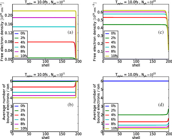
Figure 1. Dynamical properties of the irradiated carbon cluster recorded for different shells at different times, 0–10 fs, during a 10 fs-long laser pulse: (a), (c) free-electron density; (b), (d) average charge per ion, obtained for a fluence of 1011 photons per 100 nm spot per pulse (left), and for 1013 photons per 100 nm spot per pulse (right). The shells are numbered, starting from the centre of the sample.
Download figure:
Standard imageLet us note that here the outermost shell of the sample has the lowest charge. However, this is the transient charge state simulated at short times of 0–10 fs during the 10 fs long pulse. During this time, the intense photoionization of the sample takes place. Fast photoelectrons leave the sample quickly, only weakly ionizing it through collisions. As a result, the net charge of the sample is growing and the outer shell is quickly emptied of any slower electrons that are attracted towards the centre of the sample. Therefore the impact ionization process that contributes significantly to the ionization of the inner part of the sample does not further affect electrons in the outer shell. We can then observe the transient charge distribution as shown in the simulations, as the majority of ionization processes occur inside the sample. This effect can be slightly overestimated within the framework of our model, as the fast thermalization of electrons is assumed [35]. At later evolution stages the proportion of charges between the outer and the inner part of the sample will change, as the electron pressure will push more trapped electrons towards the outer shell, initiating impact ionization processes also there. On the other hand, the three-body recombination effect will be more pronounced at this time. This can significantly reduce the charge of ions within the inner part of the sample, where the density of trapped electrons is high. In this way, the sample will arrive at the final charge distribution with the outer shells ionized higher than the inner shells.
In figure 2 we show the signal intensities for the undamaged and damaged samples obtained at various pulse parameters, and the corresponding residual R-factors. These intensities (expressed in arbitrary units) are shown for different pulse fluences arriving at the sample. As the reference signal we used the signal from the undamaged sample. For the damaged case the calculated contribution of inelastic scattering was added to the calculated elastic signal. These R-factors give a global measure of signal deterioration, estimating the discrepancy between the signal recorded from the undamaged and damaged samples [29, 36]. In the R-factor plots we show for reference the limiting R-factor value of 20% obtained from x-ray crystallographic data found in protein databases [29]. As the hydrodynamic model evolves smooth electron and ion densities, and in the experiment granular ions are imaged, we accounted for the ion atomicity by convolving the ion densities obtained with the hydrodynamic model with the pair distribution function of liquid carbon [28] of density 2 g cm−3, using equation 12, and then computed the scattering signal from equation (10). This procedure was applied also for the case of the highest fluence and the longest pulse duration, as even in this case only a small fraction of ions (⩽6%) became displaced more than the maximal imaging resolution, 1 Å. We also corrected the simulation results for the effects of electron self-correlation, applying equation (9). Following the discussion at the beginning of this section, although the calculated deterioration of the signal for the considered sample is the smallest one in the case of the lowest pulse fluence of 1011 photons (focused to a 100 nm spot), the limiting value of 0.1 photon per speckle can be achieved only at fluences of the order of 1012 photons per pulse.

Figure 2. Signal intensities (left) and R-factors (right) as a function of q, obtained for a carbon cluster irradiated with a pulse of 10 fs duration at a fluence of 1011–1013 photons per 100 nm spot per pulse. The (ideal) signal intensity at the highest fluence of 1013 photons per pulse was normalized to one arbitrary unit at the lowest q value, and the lower fluence cases (1011–1012 photons) were rescaled by 100 and 10 correspondingly.
Download figure:
Standard imageWe note that including the pair distribution function in the analysis of simulation data has a large impact on the calculated scattering intensities and R-factors. For comparison, figure 3 shows the signal intensities and residual R-factors calculated directly from smooth ionic densities obtained from the simulations without convolving them with the pair distribution function. Electron self-correlations were again taken into account, equation (9). In this case the computed R-factors are much larger than in the corresponding case including the pair distribution function: the radiation damage has then a strong effect on the scattering signal. Localization of ions enforced by the pair distribution function strengthens the ionic component of the scattering signal at the high spatial frequencies around q/2π ∼ 0.1 Å−1 and reduces the overall effect of the radiation damage. Therefore, in what follows, we show only results obtained from convolving the simulation data with the pair distribution function.
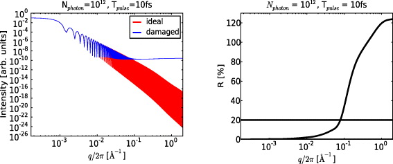
Figure 3. Signal intensities (left) and R-factors (right) as a function of q, obtained for a carbon cluster irradiated with a pulse of 10 fs duration at a fluence of 1012 photons per 100 nm spot per pulse. The data were obtained from smooth ionic densities without convolving them with the pair distribution function.
Download figure:
Standard imageWe have investigated in detail the contribution of specific damage mechanisms to the overall damage effect. Figure 4 shows signal intensities and the R-factors obtained with different damage mechanisms, when: (i) only the change of atomic scattering factors due to ionization of the sample was taken into account and the free-electron contribution was neglected, and (ii) the total signal, including also the free-electron contribution, was recorded. These estimates were obtained for a pulse length of 10 fs and a fluence of 1012 photons per 100 nm spot. In the region of low q (q/2π ⩽ 10−1 Å−1), which corresponds to high inter-particle distances, signal deterioration is caused predominantly by free electrons that are spread all over the sample. At the region of high q values (q/2π ∼ 1 Å−1), corresponding to low inter-atomic distances, the ionic damage dominates. This is the q-region where ion–ion correlations, introduced by the pair distribution function, manifest.
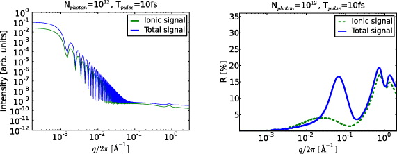
Figure 4. Signal intensities (left) and R-factors (right) (plotted as a function of q) reflecting specific damage mechanisms contributing to the signal deterioration, when: (i) only the change of atomic scattering factors due to ionization of the sample was taken into account and free-electron contribution was neglected, and (ii) total signal, including also the free-electron contribution, was recorded. These estimates were obtained for a pulse length of 10 fs and a fluence of 1012 photons per 100 nm spot.
Download figure:
Standard imageTherefore the total R-factors obtained from our analysis show characteristic maxima. The first one at low q/2π ∼ 10−1 Å−1 shows the cumulated discrepancies between the damaged and undamaged signal intensities due to the presence of the free-electron cloud. The second and third peaks reflect the discrepancies in the signal intensities in the q-region sensitive to the ion–ion correlations (q/2π ∼ 1 Å−1). These high q regions are important for high-resolution studies. For comparison, figure 5 shows the corresponding correlation peak at q/2π ∼ 1 Å−1 in the structure factor calculated for the liquid carbon. In the case of lower pulse fluence (1011 per 100 nm spot), the intensity obtained for the irradiated sample does not differ much from the ideal case (R < 10%). With increasing fluence (1011–1012 per 100 nm spot) the differences between the ideal and the damaged signal increase, however, with R-factors still reaching maximally ∼20% in the entire q region. The full set of R-factors obtained from our analysis is shown in figure 6. Again, for all the considered pulse fluences and pulse durations the R-factor remains less than or around 20% in the entire q region, which implies that the structural information about the cluster is preserved to a large extent.
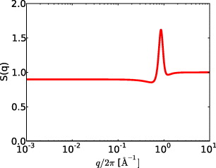
Figure 5. Structure factor calculated for liquid carbon. The pair distribution function is taken from [28].
Download figure:
Standard image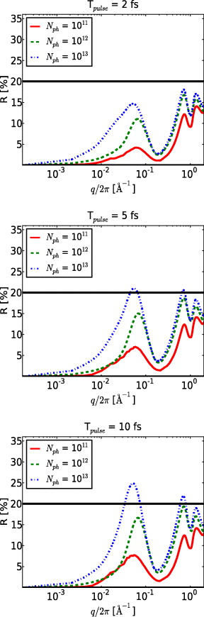
Figure 6. R-factors of the irradiated carbon cluster as a function of q, obtained at a fluence of 1011–1013 per 100 nm spot, and pulse durations 2–10 fs.
Download figure:
Standard image4. Summary
We analysed the effect of radiation damage on the structural information contained in the diffraction image of an irradiated object, a carbon cluster of 50 nm radius, which is a prototype object for CDI-related damage studies. We used hydrodynamic simulations and corrected them for the electron correlation and ion atomicity effects. We estimated also the contribution of inelastic scattering of photons on bound electrons to the scattering signal. We considered the damage due to: (i) the decrease of atomic form factors due to the progressing ionization of the sample and (ii) the scattering from the free electrons trapped within the sample. The first effect was found to be dominant in the region of high q (q/2π ∼ 1 Å−1) and the second one in the region of low q (q/2π ∼ 10−1 Å−1). The calculated R-factors did not exceed 20% at all the considered pulse durations (2–10 fs) and pulse fluences (1011–1013 per 100 nm spot) in the entire q region. This suggests that imaging at atomic resolution could be accessible at the currently available XFEL pulse parameters. However, our calculations show that in order to achieve of the order of 0.1 photon per speckle from the scattering on a 50 nm radius amorphous carbon cluster at 1 Å resolution with 1 Å wavelength x-rays, a minimum of 1012 photons must be incident on the focus spot. 3D reconstruction can then only be achieved with dedicated classification techniques that are able to handle noisy patterns [32, 33, 37–39] by analysing many patterns of the same molecule. Such an analysis will significantly improve with many-shot imaging at a high repetition rate such as will be available in the future European XFEL facility [40].
Acknowledgments
We thank Anton Barty, Veit Elser, Adrian Mancuso and Robert Thiele for useful comments and discussions. Part of this work was performed under the auspices of the US Department of Energy by the Lawrence Livermore National Laboratory under contract number DE-AC52-07NA27344.