


Abstract
We utilize a three-dimensional (3D) visible spectroscopy to reveal and explore coherent coupling between excitons localized to GaAs quantum wells separated by barriers 4 and 6 nm wide. The coupled excitons were energetically separated by 43 meV, close to the longitudinal optical phonon energy, due to the different widths of the quantum wells to which they were localized. The ability to isolate coherence pathways in 3D spectroscopy has made it possible to not only identify weak coherent coupling, but also to explore the nature of the coupling through analysis of the peak shapes. This peak shape analysis showed inhomogeneous broadening of the excitons localized to different wells to be uncorrelated, as expected, while coupling between heavy-hole and light-hole excitons localized to the same well was shown to be correlated. To gain some insight into the coupling mechanism we explored the dependence of the coupling strength on the barrier width and hence spatial separation. Based on these results we discuss the possibility of phonon-assisted dipole coupling.
Export citation and abstract BibTeX RIS

Content from this work may be used under the terms of the Creative Commons Attribution 3.0 licence. Any further distribution of this work must maintain attribution to the author(s) and the title of the work, journal citation and DOI.
1. Introduction
Coherent coupling between spatially separated quantum systems is a significant process in a number of important contexts. In the field of quantum information the ability to control coherent coupling between qubits is essential for two-qubit operations which form an important part of most proposed schemes. This same type of coherent coupling has recently been observed in the light-harvesting architecture of various natural photosynthetic organisms [1–3]. Understanding the precise mechanisms of coherent coupling in such complex condensed matter systems brings with it the possibility to control quantum states for quantum information or enhance the efficiency of directed energy transfer in future solar energy solutions.
Semiconductor quantum wells (QWs) and quantum dots have been of significant interest for studying fundamental physics and for device applications since epitaxial growth techniques were developed to produce such structures. Recent experiments exploring coherent coupling between spatially separated quantum dots have revealed strong coupling over distances up to 1 μm with very little dependence of the coupling strength on the separation [4, 5]. Such strong coupling without any discernible distance dependence cannot be explained by any of the standard coupling mechanisms such as dipole–dipole interactions, Auger decay or two-photon absorption processes. The most well-supported explanation offered to date identifies the coupling to a biexcitonic renormalization, in which the long-range nature of the coupling is attributed to the existence of spatially extended exciton states [4].
Here, we explore the coupling as a function of spatial separation between excitons localized to QWs which have different widths and hence different transition energies. These GaAs/AlGaAs asymmetric double QW (ADQW) samples were designed so that the energy difference is resonant with the longitudinal optical (LO) phonon energy in AlGaAs. This has been predicted to enhance the dipole–dipole coupling strength and increase the distance over which it can act [6]. The role and nature of phonon-assisted dipole–dipole coupling for energy transfer in natural photosynthetic systems is also becoming an important question [7–10].
In order to identify and understand coherent coupling between excitons in these ADQW samples, we use coherent three-dimensional (3D) optical spectroscopy. This technique is based on transient four-wave mixing (FWM) experiments, which have been utilized to reveal dynamics in semiconductor wells for over two decades [11–13]. The extension of transient FWM experiments to multidimensional spectroscopy has facilitated means to identify and resolve different many-body interactions in semiconductor QWs and to identify coherent coupling between different exciton states [14–20]. By extending two-dimensional (2D) spectroscopy to three dimensions further separation of different signal pathways can provide greater insight into the quantum mechanical properties of the system under investigation [21, 22]. Here we utilize 3D spectroscopy to isolate coherence pathways, which in 2D spectra are often dominated by signals from population pathways, revealing otherwise hidden couplings. By examining slices of the 3D spectrum that correspond to coherence pathways we are able not only to identify the coherences but also to access details that are otherwise extremely difficult or impossible to obtain.
2. Three-dimensional spectroscopy—techniques and advantages
In many 2D visible spectroscopy experiments much of the analysis is based on observing changes to the 2D spectrum as a function of the waiting time (the delay between the second and third pulses). It is typically assumed that over this waiting time the system is in a population state with no phase evolution. Recently, however, there has been considerable interest in coherent superpositions of excited states, which do have some phase evolution over this waiting time. Indeed, such oscillations have been used as the primary evidence for long-lived coherences in photosynthetic light harvesting complexes at room temperature [2, 3]. Previous work has fitted each point in the 2D spectrum to exponentially decaying oscillating functions of waiting time, as a means of gaining insight into the properties of these coherences, such as their decay times and the relative contributions of inhomogeneous broadening [23, 24]. To further understand the nature and properties of this type of coherent evolution, however, it is desirable to separate these coherence pathways from population pathways, which have components that overlap in the 2D spectra. One way of achieving this is to perform narrow-band two-colour experiments, to excite specifically the coherence pathways [8, 25, 26], though this limits the temporal resolution. Alternatively, a Fourier transform of the data with respect to the waiting time will generate a 3D spectrum with the coherence pathways separated from the population pathways [3, 17, 19, 21, 22]. This type of 3D spectrum is quite distinct from other 3D spectroscopies that have been reported, such as 3D spectra that involve a two-quantum coherence or the 3D spectra in infrared spectroscopy that plot data against three one-quantum axes from fifth-order experiments [27, 28].
A slice from the 3D spectrum in the (ωτ,ωt) plane at the value of ωT corresponding to the coherence frequency resembles a familiar 2D spectrum. To understand the nature of such a slice we turn to the projection slice theorem, which is commonly used to compare traditional 2D spectra to pump–probe data. This tells us that a projection of the 3D spectrum along the ωT axis is equivalent to the 2D slice at T = 0. Similarly, the projection along the T-axis would give the 2D-spectrum at ωT = 0. Furthermore, if a phase shift is added as a function of T then a slice at any value of ωT can be obtained from the projection along T, depending on the phase shift. In other words, a single 2D slice at a given value of ωT represents the component of the data oscillating at that frequency, integrated over the range of T. By examining such slices we overcome some of the problems of analysing coherence pathways in standard 2D spectra. For example, in standard 2D spectra the phase of coherence peaks evolve as the value of T is varied, making it difficult to determine the peak properties such as peak shape. This is not a problem in such a 2D slice of the 3D spectrum, allowing standard peak shape analysis tools to be applied. For example, a peak elongated along the diagonal indicates inhomogeneous broadening of the two states in the coherent superposition that is correlated, whereas a round peak indicates that if there is any inhomogeneous broadening of the two states then it is uncorrelated [22].
Just as the electronic transitions excited by the laser pulses have finite line widths, so too do the coherent superpositions. This leads to peaks that are not necessarily confined to a single 2D plane, but which extend over the range of the line width. Furthermore, it is expected that the peak shape in the 2D slice will change as we move away from the centre of the peak along the ωT axis, much like the phase of a peak changes in a 2D spectrum as one moves away from the centre (except along the diagonal). Calculations based on a three-level system with correlated inhomogeneous broadening [29] demonstrate this expected behaviour. Figures 1(a) and (b) show the real rephasing part of the calculated 3D spectrum from different perspectives, while slices of the 3D spectrum are shown in (c)–(g) at ωT = −0.06, 0.06, −0.001, 0 and 0.001 eV, respectively. These plots reveal that a typical absorptive lineshape is seen in 2D slices at the centre of a peak on the ωT axis (c), (d), (f). As we move along the ωT axis, however, dispersive lineshapes become apparent (e), (g), with a π phase shift in data obtained on one side of the peak centre relative to the other. From the 3D spectrum it can also be seen that a line can be defined which is equivalent to the diagonal in a 2D spectrum for which the phase of the peak remains zero.
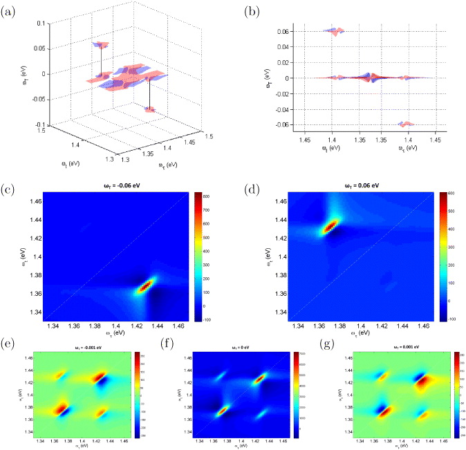
Figure 1. Panels (a) and (b) show the real part of the rephasing 3D spectrum presented as an isosurface viewed from two different angles. The red isosurface indicates positive values, while the blue is negative. Panel (b) shows the perspective looking down the diagonal of the (ωτ,ωt) plane. Slices of the 3D spectrum are shown in (c)–(g) at ωT = −0.06, 0.06, 0.001, 0 and 0.001 eV, respectively.
Download figure:
Standard image High-resolution imageFigures 1(c) and (d) show the real part of the slices at ±0.06 meV, corresponding to the maximum of the coherence peak. As these data contain only the rephasing contributions, only cross-peaks arising from coherence pathways are present (non-rephasing spectra are shown in the supplementary material, available from stacks.iop.org/NJP/15/045028/mmedia). These peaks are both elongated along the diagonal, as expected for the correlated inhomogeneous broadening that has been introduced. Both peaks also show positive absorptive peak shapes that are indicative of the stimulated emission type pathway. In contrast, if the peaks were negative, this would indicate an excited state absorption from the coherent superposition of states. These details only become evident by examining the 3D spectrum or slices of them, and cannot easily be determined simply by following the signal evolution as a function of T.
3. Sample details
We report here results from three samples, each consisting of two GaAs QWs 5.7 and 8.0 nm wide, separated by Al0.35Ga0.65As barriers 4, 6 and 20 nm wide. We calculated the eigenstates for electrons in the conduction band and light- and heavy-holes in the valence band by solving the one-dimensional Schrödinger equation for the potential profiles in the growth direction. Numerov's method is used to determine the wavefunctions from the Schrödinger equation in conjunction with the shooting method with bisection to determine the eigenenergies. The effective masses in GaAs were taken to be 0.067, 0.51 and 0.082me for, respectively, the electron (E), heavy-hole (HH) and light-hole (LH), where me is the free electron mass. The band gaps of GaAs and Al0.35Ga0.65As were taken to be 1.51 and 1.93 eV, respectively, with a conduction band offset of 280 meV. These calculations neglect Coulomb interactions between the particles and hence the exciton binding energy, which we expect to be ∼10 meV. Regardless, the purpose of these calculations is not to give a precise calculation of the transition energies but, rather, to determine wavefunction overlaps and transition probabilities. The results of these calculations and the defining potentials are plotted in figure 2.

Figure 2. The quantum well profiles of each of the samples investigated, together with the calculated wavefunctions for electrons in the conduction band and LHs and HHs in the valence band.
Download figure:
Standard image High-resolution imageThe calculations show that each of the E, HH and LH wavefunctions are localized to a single quantum well for the sample with the 20 nm wide barrier. The HH wavefunctions are also well-localized to the individual QWs for the sample with the 4 and 6 nm wide barriers but there is a significant tunnelling probability for the LHs. In order to assess the extent of localization we calculate the probability of finding each of the wavefunctions on the other side of the centre of the barrier (see table 1). These values confirm that the HHs are well localized, even for the 4 nm barrier, whereas the LHs have a much greater probability of tunnelling into the other well and the electrons in the conduction band have a finite but small probability of tunnelling, which becomes less than 0.3% with 6 nm barriers.
Table 1. The probability of finding each particle in either QW.
| Wavefunction | Barrier (nm) | Wide well | Narrow well (%) |
|---|---|---|---|
| HHw | 4 | 99.998% | 0.002 |
| 6 | 100% | 0.0001 | |
| 20 | 100 | 0 | |
| HHn | 4 | 0.01% | 99.990 |
| 6 | 0.0006% | 99.9994 | |
| 20 | 0 | 100 | |
| LHw | 4 | 95.7% | 4.3 |
| 6 | 99.2% | 0.2 | |
| 20 | 100% | 0 | |
| LHn | 4 | 5.8% | 94.2 |
| 6 | 1.4% | 98.6 | |
| 20 | 0 | 100 | |
| Ew | 4 | 98.8% | 1.2% |
| 6 | 99.86% | 0.14% | |
| 20 | 100% | 0 | |
| En | 4 | 1.8% | 98.2% |
| 6 | 0.3% | 99.7% | |
| 20 | 0 | 100% |
As a result of the tunnelling, spatially indirect transitions involving an electron state predominantly localized in one well and a hole state localized in the other well become increasingly probable. The transition probability is directly proportional to the electron–hole wavefunction overlap, which in the case of the 4 nm barrier gives values around 10% of the spatially direct transitions for each of the spatially indirect transitions. For the 6 nm barrier these transition probabilities reduce to ∼5% for the LH indirect transitions and ∼3% for the HH indirect transitions. A table with all calculated transition energies and wavefunction overlaps is presented in the supplementary material (available from stacks.iop.org/NJP/15/045028/mmedia). We use these calculations to support the interpretation of the experimental results.
4. Experimental results
We perform coherent multidimensional spectroscopy as described previously [22, 30, 31] on each of the samples at a temperature of 20 K. In each of the samples four peaks corresponding to the four spatially direct transitions can be observed and are attributed, in order of increasing energy, to the HH exciton localized to the wide well (HHw), the LH exciton localized to the wide well (LHw), the HH exciton localized to the narrow well (HHn) and the LH exciton localized to the narrow well (LHn). These peaks are spectrally spread over ∼80 meV, which is greater than the bandwidth achievable with our laser system (Spectra Physics Tsunami). We have therefore conducted experiments with the laser spectrum centred to excite the three lowest energy transitions and in some cases resonant with the two highest energy transitions. In all experiments the laser pulses were co-linearly polarized with 250 ± 50 nJ cm−2 per pulse, exciting ∼1010 excitons per well cm−2. Frequency-resolved optical gating measurements revealed the pulses to be ∼60 fs long, and nearly transform-limited in all cases.
Figure 3(a) shows the 2D spectrum from the sample with the 4 nm barrier with a waiting time, T = 0. In figure 3(b) the projection of the 2D spectrum onto the ωt detection energy axis reveals three peaks corresponding to the HHw, LHw and HHn transitions as labelled. The relative amplitudes of these peaks is due to the convolution of the oscillator strengths with the exciting laser spectrum shown. Peaks on the diagonal from each of these three transitions can be identified in the 2D spectrum. The strong peak at ∼1.615 eV from the HHn exciton is elongated along the diagonal, as expected for an inhomogeneously broadened transition. The two weaker peaks at 1.57 and 1.59 eV due to the HHw and LHw transitions, are elongated along the ωτ axis. This stretching along the ωτ axis is a reflection of the very rapid dephasing of these excitons caused by the excitation and subsequent scattering of free-carriers in the wide well [32–34]. The HHn exciton does not display this behaviour because the excitation spectrum does not extend to sufficiently high energy to excite free-carriers in the narrow well. This suggests that the effects of the free-carriers in the wide well on the HHn exciton is minimal, despite the calculations that show finite probability for the tunnelling of the predominantly wide well electron and LH states. This also suggests that the different carriers are all well-localized and that spatial overlap is minimal, even in the sample with a 4 nm barrier.
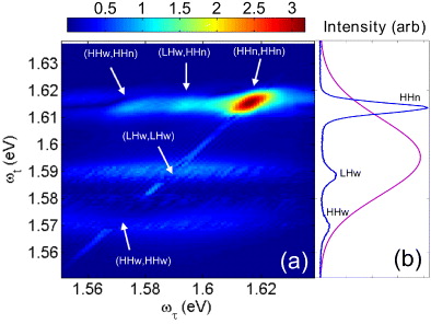
Figure 3. For the sample with the 4 nm barrier (a) the absolute value 2D spectrum at T = 0 for the rephasing part of the data with asinh colour scaling. (b) The projection of the 2D plot onto the ωt axis, which reveals three peaks corresponding to HHw, LHw and HHn, as labelled. The oscillator strengths of these transitions are convoluted with the laser spectrum shown to give the relative peak heights.
Download figure:
Standard image High-resolution imageIn addition to the diagonal peaks, some cross-peaks with emission at the HHn energy are also present. It is, however, difficult to resolve separate peaks in this amplitude 2D spectrum at T = 0. Figure 4 shows the real part of the 2D spectrum at four different time delays. In each case, the diagonal peak from the HHn exciton exhibits an almost dispersive line-shape, as has been seen previously [14, 15]. This deviation from the expected absorptive peak-shape is attributed to many-body effects such as excitation-induced shift and excitation-induced dephasing. The cross-peak with absorption at the HHw energy (ωτ = 1.57 eV) is predominantly positive, suggesting a stimulated emission or ground state bleach signal pathway. As the waiting time delay is changed, however, the profile of the peak changes. By 20 fs the peak exhibits more of a dispersive profile, at 40 fs the peak is negative and at 90 fs the peak is predominantly positive again. This temporal oscillation in the phase of the peak continues out to at least 250 fs, as can be seen in the movie in the supplementary material (available from stacks.iop.org/NJP/15/045028/mmedia). These phase oscillations make the identification of the peak shape and nature of the signal pathway very difficult. Similarly the cross-peak with absorption at the LHw exciton energy (ωτ = 1.59 eV) fluctuates as a function of waiting time, though the phase oscillations are less clear.
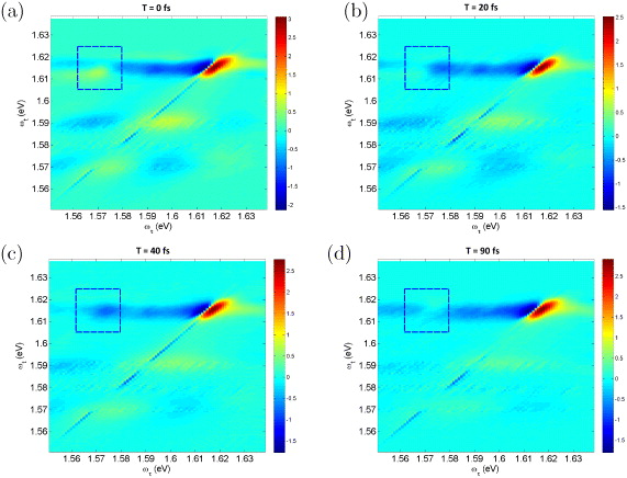
Figure 4. The real 2D spectra of the rephasing part of the data from the ADQW sample with a 4 nm barrier at waiting times of (a) 0, (b) 20, (c) 40 and (d) 90 fs. An arcsinh colour scaling is used to highlight the low-amplitude parts of the signal and allow the phase evolution of the cross-peak (indicated by the box in each spectrum) to be seen.
Download figure:
Standard image High-resolution imageBy performing the Fourier transformation with respect to T the 3D spectrum shown in figure 5 is obtained, which shows contributions from both cross-peaks that have been separated along the ωT axis, indicating signal pathways that go via a coherence during the waiting time, T. Slices of the real parts of the 3D spectrum are shown in figure 6. The slice at ωT = 46 meV shows the enhanced cross-peak at (ωτ,ωt) = (HHw, HHn) = (1.57 eV, 1.615 eV). This peak shows no elongation along the diagonal direction, as indicated by the peak width along the diagonal (8.5 ± 0.5 meV) and anti-diagonal (7.6 ± 0.5 meV) directions (see supplementary material for fitting details). This symmetric peak shape is indicative of uncorrelated inhomogeneous broadening [22]. In the real part a positive absorptive profile is apparent, as expected for the Raman-like coherence pathway. Given that the inhomogeneous broadening is predominantly due to interface fluctuations and defects, which are different for the different wells, broadening that is not correlated between the different wells is expected. In contrast, the coherence between HH and LH excitons in the same well should experience much the same inhomogeneous broadening and thus lead to coherence peaks that are elongated along the diagonal direction.
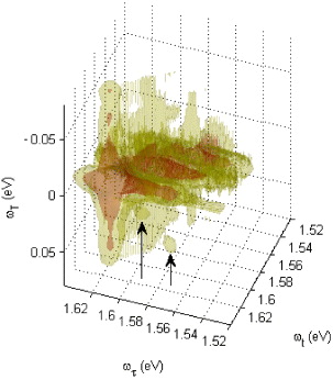
Figure 5. The 3D spectrum showing isosurfaces of the amplitude from the sample with 4 nm barriers. Modified from [22].
Download figure:
Standard image High-resolution image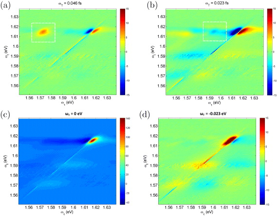
Figure 6. Slices of the 3D spectrum from the sample with 4 nm barriers showing the real rephasing contribution at ωT = (a) 46, (b) 23, (c) 0 and (d) −23 meV. The cross-peaks discussed in the text have a box around them. Each slice covers a range of 7 meV along the ωT axis.
Download figure:
Standard image High-resolution imageIn figure 6 cross-peaks due to coupling between the HHw and LHw excitons cannot be resolved due to the free-carrier contribution and rapid dephasing of the excitons in the wide well. Figure 7 shows slices of the 3D spectrum when the laser spectrum was shifted to excite just the HHn and LHn transitions. In this case the cross-peaks amplitudes are much larger than those in figure 6 due to the greater coupling strength. The slice at ωT = 24 meV shows the cross-peak elongated along the diagonal, with diagonal width 6.6 ± 0.3 meV and anti-diagonal width 4.4 ± 0.3 meV, indicating strongly correlated inhomogeneous broadening (see supplementary material, available from stacks.iop.org/NJP/15/045028/mmedia for fitting details). The slice at ωT = −24 meV shows the conjugate cross-peak enhanced, although the total amplitude is significantly lower due to the lower LH oscillator strength. These two cross-peaks, above and below the diagonal, evolve with conjugate coherent superpositions over the waiting time so that they are at conjugate points on the ωT axis, as well as being at conjugate points in the (ωτ,ωt) plane.
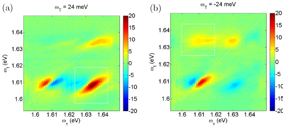
Figure 7. Slices of the real value 3D spectrum of the rephasing part of the data recorded when the laser pulse was resonant with the LHn and HHn transitions only. Slices covering a range of 7 meV are shown at (a) ωT = −24 meV and (b) ωT = 24 meV, where conjugate cross-peaks are enhanced and show positive peaks elongated along the diagonal, indicative of correlated inhomogeneous broadening.
Download figure:
Standard image High-resolution imageIn figure 6 only the 'above-diagonal' cross-peaks are present. We attribute this to the weak third-order emission from the excitons localized to the wide well due to the rapid dephasing caused by unbound electrons and holes. This type of asymmetry in cross-peaks has been observed previously and similarly explained by a combination of many-body effects and different dephasing times [18, 36]. In the discussion that follows we consider only this above-diagonal cross-peak and its properties.
The slice of the 3D spectrum in figure 6(b) at ωT = 23 meV shows the enhanced cross-peak at (ωτ,ωt) = (LHw,HHn) = (1.59 eV,1.615 eV). In this case however, the cross-peak is negative. This suggests an excited state absorption from the coherence to the mixed biexciton state. The presence of a biexciton involving excitons localized to different wells may initially seem unexpected but it becomes more likely because of the presence of strong coupling, which is evidenced by the presence of the coherent superposition. It is not clear, however, why the biexciton pathway appears to dominate over the stimulated emission (stimulated Raman) pathway, which would give a positive peak.
Further evidence for the presence of biexcitons is apparent in the slice at ωT = 0 in figure 6. In this real rephasing spectrum there are cross-peak signals present in the region around the absorption energies corresponding to HHw and LHw excitons and emission at the HHn energy. All of this signal is negative, however, indicating excited state absorption and the presence of biexcitons. In contrast, the presence of any positive cross-peak in this slice at ωT = 0 would be indicative of a shared ground state between the HHn exciton and the LHw or HHw exciton. The absence of such a signal provides confirmation that the spatially direct excitons are indeed well localized to the individual QWs, yet coherent coupling between excitons localized to different wells is present.
An alternative possibility that we consider is that the observed coherence cross-peaks are not actually due to coupling between two spatially direct excitons but due to coupling between one spatially direct exciton and a spatially indirect exciton that shares either an electron or hole state with the direct exciton. Table S1 in the supplementary material (available from stacks.iop.org/NJP/15/045028/mmedia) shows that several indirect excitons are relatively bright, with transition probabilities 10% of the direct excitons, and transitions energies close to those of the direct excitons. This would provide a clear mechanism for the coupling; if this were the case, however, positive cross-peaks in the slice at ωT = 0 would be expected but they are not seen.
There are several possible mechanisms for the coherent coupling of these spatially separated excitons, including dipole–dipole interactions, which are expected to be short-range, intrinsic structural inhomogeneity in the barriers, Auger processes and two-photon absorption processes. In an attempt to clarify the mechanism responsible for the observations we have repeated these measurements for the samples with 6 and 20 nm barriers.
The 2D spectra from these samples at T = 0 are shown in figure 8. The overall appearance of these spectra is much the same as for the sample with the 4 nm barrier. A strong diagonal peak is observed due to the HHn exciton, together with two weaker and lower energy peaks on the diagonal from the HHw and LHw excitons that are stretched along ωτ due to scatter from the free-carriers excited in the wide well. In both cases there is also some signal in the cross-peak region, but again, it is difficult to discern clear peaks and impossible to say whether or not there is any clear coherent coupling between spatially separate excitons.
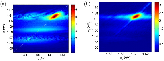
Figure 8. The 2D spectra at T = 0 fs for the samples with (a) 6 nm and (b) 20 nm barriers.
Download figure:
Standard image High-resolution imageThe slices from the 3D spectra at ωT = 46 and 23 meV are shown in figure 9. In both cases there is no apparent cross-peak in the slice at ωT = 23 meV. In the sample with 6 nm barriers, however, there is a weak but clear cross-peak corresponding to absorption at the HHw transition and emission at the HHn transition energy. This coherence cross-peak is very weak and as a result the low signal to noise makes determining the peak shape difficult. Nonetheless, there is clearly a peak here which is indicative of coherent coupling between spatially separated excitons (slices at other values of ωT are shown in the supplementary material (available from stacks.iop.org/NJP/15/045028/mmedia) to confirm that this peak is isolated along the ωT axis).

Figure 9. Slices covering a range of 7 meV along the ωT axis from the 3D spectra for the samples with the 6 nm barrier (a), (b) and 20 nm barrier (c), (d). At values of ωT = 23 meV no clear cross-peaks are seen in either sample (a), (c). At ωT = 46 meV, (b), a cross-peak can be seen in the sample with a 6 nm barrier.
Download figure:
Standard image High-resolution image
To gain an estimate of the relative coupling strength we integrate the signal amplitude of the cross-peak in the slice at ωT = 46 meV and the diagonal peak in the slice at ωT = 0. With the 4 nm barrier the integrated HHw/HHn coherence cross-peak amplitude is 10% of the integrated amplitude of the HHn diagonal peak. For the 6 nm barrier this ratio has been reduced to ∼2%. In both cases this fraction is much greater than the calculated probability of finding the HH in the other well, and substantially more than the electron tunnelling probability. Furthermore, if the coupling were in some way dependent on the extent of wavefunction tunnelling, then coupling between the LHw and HHn excitons would be expected to be greater than the HHw/HHn coupling because of the much greater tunnelling probability of the LH. In both the 4 and 6 nm barriers this is not the case and the opposite is true.
Dipole–dipole coupling is expected to exhibit a very rapid fall off with spatial separation. As the barrier was increased from 4 to 6 nm the coupling strength did decrease substantially. The dipole coupling strength is, however, also expected to fall off as the energy separation increases, again suggesting that the LHw/HHn coupling should be stronger. In the case of phonon-assisted dipole coupling, however, this need not be the case, and the spatial range of the coupling can be enhanced [6]. For this to be a feasible mechanism the energy separation of the 1s levels needs to be equal to the LO-phonon energy [6]. The energy separation in this case is ∼43 meV, which is close to the LO-phonon energy in Al0.35Ga0.65As (39 meV). When considering phonon-assisted processes there are two possibilities. In the case considered by Batsch et al [6] the energy transfer between QWs separated by the LO-phonon energy is greatly enhanced, but is incoherent [18]. Coherent interactions between phonons and excitons are, however, possible [35] and one may conceive a coherent dipole coupling between one exciton and another exciton coupled to an LO-phonon. This type of process would suggest that coherent phonons may be required. Another possible coupling mechanism is structural inhomogeneity in the barrier where channels of low potential are created by microscopic clustering of like molecules, which enables percolation-like transport processes [18, 37].
Finally, we have so far focused on the cross-peaks and the role of coupling between excitons localized to different wells. The slices of the 3D spectrum can also help reveal the different many-body effects through the line-shape of the diagonal peaks. In the simulations without many-body effects the slice at ωT = 0 shows a positive absorptive peak profile and at other values of ωT it has a dispersive peak shape, with opposite phase depending on which side of ωT = 0 it is. The phenomenological inclusion of many-body effects changes these profiles, effectively introducing a phase shift across the peak and some elongation in the ωτ and/or ωt directions, depending on the type of excitation induced effect. Similarly, excitation induced effects that depend on exciton populations, as opposed to polarizations, will introduce some additional waiting time dependence and hence some extension of the diagonal peak in the ωT direction. Recent work has identified that both population and polarization induced many-body effects are important [38] and this presents a possible means of separating the different contributions. A full and detailed description of how different many-body effects can be identified in slices of the 3D spectrum will be the topic of future work.
5. Summary
We have detailed several properties of 3D visible spectra and demonstrated some of the unique benefits. This technique provides an important additional means to separate different signal pathways and allows analysis that is otherwise complicated by overlapping and oscillating signals.
By examining slices of the 3D spectrum from ADQWs we have been able to identify coherent coupling between spatially separated excitons and identify the uncorrelated nature of the inhomogeneous broadening. In the same manner we have identified coherent coupling between HH and LH excitons localized in the same well, with inhomogeneous broadening that is correlated.
The coherent coupling between the HH excitons localized to the two different wells became substantially weaker as the barrier width was increased from 4 to 6 nm and was not observed when the barrier was 20 nm wide. This strong separation dependence is consistent with several possible coupling mechanisms. The 43 meV energy separation of the two excitons suggests a possible role for coherent phonons, perhaps in the form of phonon-mediated dipole–dipole coupling. To clearly identify the coupling mechanism, however, further work exploring the dependence on energy and spatial separation of the excitons is required.
Acknowledgments
We thank A/Professor Hoe Tan and Professor Jagadish for providing the samples and the Australian National Fabrication facility for providing the growth facilities. We also acknowledge support from the Australian Research Council Discovery Projects and Future Fellowship schemes.