Continuum theory of gene expression waves during vertebrate segmentation

In all vertebrate animals, the segmentation of the body plan proceeds during embryonic development in a process termed somitogenesis [1]. During somitogenesis, the elongating body axis segments rhythmically and sequentially into somites, the precursors of vertebrae and ribs. Failure of proper segmentation, caused for instance by mutations, can give rise to birth defects such as congenital scoliosis [2]. Somites are formed in characteristic time intervals from an unsegmented progenitor tissue, the presomitic mesoderm (PSM) (figure 1(A)). The temporal regularity with which somites form has provoked the idea that a biological clock comprised of cellular oscillators coordinates the temporal progress of segmentation in the PSM. The so-called 'clock-and-wavefront' mechanism suggests that a wavefront at the anterior end of the PSM reads out the state of this clock and triggers the formation of a new segment upon each completed clock cycle [3]. Indeed, patterns of oscillating gene expression have been found in the PSM of various vertebrates such as zebrafish, chick, mouse, frog, and snake [1]. These patterns resemble traveling waves sweeping through the PSM and occur as a result of coordinated cellular oscillations in the concentration of gene products (figure 1(B)). Genetic oscillations are proposed to occur autonomously in single cells as a result of delayed autorepression of specific genes [5, 6]. Cellular oscillators mutually couple through Delta–Notch signaling between neighboring cells, which tends to locally synchronize their oscillatory dynamics [7–11]. Local synchronization due to coupling is important to maintain coherent wave patterns by preventing the cellular oscillators from drifting out of phase due to noise in gene expression [12–14]. The emergence of traveling waves at the tissue level has been linked to a gradual slowdown of genetic oscillations in the PSM along the body axis [1, 13, 15, 16]. This gradual slowdown corresponds to a spatial profile of intrinsic frequencies of the cellular oscillators.

Zoom In Zoom Out Reset image size

During segmentation, the waves of gene expression emerge at the posterior of the PSM and travel towards its anterior end, where the new segments are formed (figure 1(B)). Segment formation occurs upon arrival of a wave at the anterior end of the PSM. This corresponds to the formation of one segment with each completed oscillation cycle at the anterior end [4]. Segmentation is a highly dynamic process: in parallel with segment formation, the body axis elongates while at the same time PSM changes its length as cells leave the PSM at the anterior end to form somites [4, 16]. A shortening of the PSM, as observed in Zebra fish moves relative to the waves giving rise to a Doppler effect (figure 1(C)) [4]. The motion of the anterior end relative to the posterior tip leads to an increase of the frequency of oscillations seen by an observer at the anterior end. Since the oscillation frequency at the anterior end specifies the rate of segmentation, this Doppler effect contributes to a decrease of the period of morphological segment formation. In addition to the Doppler effect, the wavelength of the pattern dynamically changes over time. This leads to a modulation of the local frequency and contributes to an increase of the period of segmentation. Together, both effects combine to determine the timing of segment formation. Hence, in addition to the time scale of genetic oscillations, the rate of segment formation is regulated by the time scale set by tissue shortening and the wavelength of the wave pattern. These observations highlight the need to capture the effects of tissue deformation in theories of vertebrate segmentation.

In this paper, we present a minimal continuum theory of vertebrate segmentation based on coupled phase oscillators in a dynamic medium that takes into account local growth and shortening of the oscillating tissue during the segmentation process. In section 2, we introduce our continuum theory of vertebrate segmentation and the key observables that can be obtained from the theory. In section 3, we illustrate the basic mechanism of pattern formation with oscillators using a simplified scenario with constant length of the oscillating tissue. In section 4, we apply our theory to quantitatively describe segmentation in developing zebrafish embryo, taking into account tissue shortening. In section 5, we discuss the factors that regulate the period of segmentation and show how a Doppler effect and a dynamic wavelength effect emerge from the interplay of tissue shortening and changing wave patterns. In section 6, we discuss our findings and give an outlook for further research.

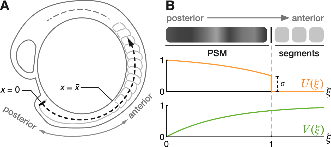
Here we introduce a theory that aims to describe the wave patterns in the PSM and the dynamic features of segmentation that result from these wave patterns. The wave patterns and the timing of segmentation have previously been quantified in transgenic zebrafish embryos, in which oscillating genes have been tagged with a fluorescent marker protein [4]. Waves can be traced by introducing a one-dimensional coordinate x along the curved embryonic body axis and measuring the fluorescent intensity level along this axis over time (figures 1(B) and 2(A)). Since these wave patterns are a tissue-level phenomenon and phase differences between neighboring cellular oscillators are typically small, we here choose a coarse-grained continuum description of the oscillatory medium. We describe the local state of oscillation by a phase field $\phi (x,t).$ Our theory combines three key ingredients involved in pattern formation during vertebrate segmentation: (i) autonomous oscillators with a spatial profile $\omega (x)$ of intrinsic frequencies [13, 15], (ii) local oscillator coupling with strength [10, 13], and (iii) a cell velocity field v(x) capturing deformation and elongation of the segmenting body axis [17, 18]. The dynamic equation for the phase field ϕ is given by [13]

$$\begin{eqnarray}&&\displaystyle \frac{\partial \phi }{\partial t}+v\displaystyle \frac{\partial \phi }{\partial x}=\omega +\displaystyle \frac{\varepsilon }{2}\displaystyle \frac{{\partial }^{2}\phi }{\partial {x}^{2}}.\end{eqnarray} \tag{ 1 }$$

The intrinsic frequency of the oscillators is described by a position-dependent frequency profile $\omega (x).$ Motion of the cellular oscillators is described by an advective term where v is the cell velocity. In previous work, we have considered a constant velocity v. Local oscillator coupling with strength is described by a term that tends to even out local phase differences and thus describes the oscillators' tendency to locally synchronize [19]. We impose open boundary conditions, $(\partial \phi /\partial x){| }_{x=0}=0,$ which corresponds to the situation where there are no oscillators beyond the posterior tip.

In order to describe a shortening PSM, we consider the simple case where the frequency and the velocity profile are rescaled with tissue length

$$\begin{eqnarray}&&\omega ={\omega }_{0}U(x/\bar{x}(t)),\end{eqnarray} \tag{ 2 }$$

$$\begin{eqnarray}&&v={v}_{0}V(x/\bar{x}(t)),\end{eqnarray} \tag{ 3 }$$

where U and V are spatial profiles that are adjusted to the variant length $\bar{x}(t)$ of the PSM, ${\omega }_{0}$ is the maximum frequency at the posterior tip x = 0, and v₀ is a typical velocity.

Phase waves travel in an anterior direction if the frequency profile attains its maximum frequency at the posterior tip x = 0 and decays in an anterior direction [13, 15]. For simplicity, we consider that oscillations have ceased beyond the wavefront and therefore choose the following frequency profile

$$\begin{eqnarray}U(\xi )=\left\{\begin{array}{ll}\sigma +(1-\sigma )\displaystyle \frac{1-{{\rm{e}}}^{k(\xi -1)}}{1-{{\rm{e}}}^{-k}} & \xi \leqslant 1\\ 0 & \xi \gt 1,\end{array}\right.\end{eqnarray} \tag{ 4 }$$

see figure 2(B), where $\xi =x/\bar{x}$ denotes a non-dimensional position coordinate and k⁻¹ is a characteristic (non-dimensional) length scale of the profile. The function U has the boundary values $U(0)=1$ and $U(1)=\sigma$ (figure 2(B)).

Zoom In Zoom Out Reset image size

The velocity field in the segmented region can be estimated from experiments by tracking the velocity of segment boundaries, see appendix A. Choosing the boundary condition $v(0)=0,$ a simple choice for the velocity profile consistent with the quantified data is

$$\begin{eqnarray}&&V(\xi )=1-{{\rm{e}}}^{-q\xi },\end{eqnarray} \tag{ 5 }$$

see figure 4(B). The velocity gradient v corresponds to local growth rate with a profile $\partial v/\partial x=({{qv}}_{0}/\bar{x}){{\rm{e}}}^{-{qx}/\bar{x}}$ that takes its maximum value at the posterior tip x = 0 and decays over the characteristic length scale $\bar{x}/q.$ The choice of the functional forms for U and V are motivated by experimental observations as they give rise to the type of wave patterns observed in experiments with waves moving in anterior direction and slowing down as they approach the anterior end, see section 3.

Zoom In Zoom Out Reset image size

Zoom In Zoom Out Reset image size

The number of waves that simultaneously sweep through the PSM is a key observable that can be measured in experiments [1]. In terms of the phase field ϕ, the number of waves K(t) is given by

$$\begin{eqnarray}&&K(t)=\displaystyle \frac{\phi (0,t)-\phi (\bar{x}(t),t)}{2\pi }.\end{eqnarray} \tag{ 6 }$$

Hence, $2\pi K$ is the total phase difference between the posterior tip x = 0 and the anterior end $x=\bar{x}$ of the PSM. A new segment is formed after each completed oscillation cycle at the anterior end $x=\bar{x}$ [4]. Accordingly, the number of formed segments at time t is given by

$$\begin{eqnarray}&&N(t)=\displaystyle \frac{\phi (\bar{x}(t),t)}{2\pi }\end{eqnarray} \tag{ 7 }$$

and the rate of segment formation is ${\rm{d}}N/{\rm{d}}t.$ The length S of the formed segments at the time t of their formation is given by the wavelength of the pattern at the anterior end, and obeys $| \phi (\bar{x},t)-\phi (\bar{x}+S(t),t)| =2\pi .$ In the case where $\partial \phi /\partial x$ does not vary strongly over the length S, the segment length can be approximated as

$$\begin{eqnarray}&&S(t)\simeq \displaystyle \frac{2\pi }{\left|\displaystyle \frac{\partial \phi }{\partial x}(\bar{x}(t),t)\right|}.\end{eqnarray} \tag{ 8 }$$

We first discuss time-periodic patterns to illustrate how the properties of the wave pattern depend on the parameters of our theory. Such patterns occur for constant PSM length, $\bar{x}(t)={\bar{x}}_{0}.$ Figure 3(A) shows a kymograph of a time-periodic solution to equation (1). Starting with $\phi (x,t=0)=0,$ the system attains a time-periodic state after transient dynamics. This time-periodic state can be expressed in the form [13, 19]

$$\begin{eqnarray}&&\phi (x,t)={\rm{\Omega }}t+\psi (x),\end{eqnarray} \tag{ 9 }$$

where Ω is the collective frequency and the spatiotemporal pattern $\mathrm{sin}\phi (x,t)$ is fully characterized by the time-independent phase profile $\psi (x).$ The rate of segment formation ${\rm{d}}N/{\rm{d}}t,$ defined through equation (7), is given by ${\rm{d}}N/{\rm{d}}t={\rm{\Omega }}/2\pi$ and hence given by the collective frequency. Using the time-periodic ansatz equation (9) in equation (1), the phase profile ψ obeys the ordinary differential equation

$$\begin{eqnarray}&&{\rm{\Omega }}+v{\psi }^{\prime }=\omega +\displaystyle \frac{\varepsilon }{2}{\psi }^{\prime\prime }\end{eqnarray} \tag{ 10 }$$

with boundary condition ${\psi }^{\prime }(0)=0.$ It is instructive to consider the case of weak coupling, in which the coupling term provides only a minor correction to the collective frequency and the phase profile (figure 3(B)). Neglecting $(\varepsilon /2){\psi }^{\prime\prime }$ in equation (10), we find the collective frequency ${\rm{\Omega }}\simeq {\omega }_{0},$ the maximum of the frequency profile at the posterior tip. The phase profile ψ can then be approximated as

$$\begin{eqnarray}&&\psi (x)\simeq {\displaystyle \int }_{0}^{x}\displaystyle \frac{\omega (x^{\prime} )-{\rm{\Omega }}}{v(x^{\prime} )}\;{\rm{d}}x^{\prime} .\end{eqnarray} \tag{ 11 }$$

Figure 3(B) shows the approximation equation (11) together with the phase profile obtained from a numerical solution of equation (1) including the effects of coupling. The number of waves that simultaneously sweep through the PSM is given by $K=| \psi ({\bar{x}}_{0})| /2\pi .$ The length S of formed segments is constant and given by equation (8) as

$$\begin{eqnarray}&&S=\displaystyle \frac{2\pi }{| {\psi }^{\prime }({\bar{x}}_{0})| }\simeq {v}_{0}T,\end{eqnarray} \tag{ 12 }$$

where we have approximated $v({\bar{x}}_{0})\simeq {v}_{0}$ and defined the collective period $T=2\pi /{\rm{\Omega }}.$ This relationship is well-known from the clock-and-wavefront model [3, 13]. Note that in the case of a velocity profile it only holds approximately and only for time-periodic solutions. The phase velocity $\tilde{v}={\rm{d}}{x}_{*}/{\rm{d}}t$ of the waves can be obtained as the velocity of a point x_* with constant phase, $\phi ({x}_{*}(t),t)={\phi }_{*}$ [20]. Differentiating this relation with respect to time yields the phase velocity $\tilde{v}=-(\partial \phi /\partial t)/(\partial \phi /\partial x){| }_{x={x}_{*}(t)},$ which exists at any position x. Using equations (9) and (11), we obtain

$$\begin{eqnarray}&&\tilde{v}(x)\simeq \displaystyle \frac{v(x)}{1-\omega (x)/{\omega }_{0}}.\end{eqnarray} \tag{ 13 }$$

The phase velocity $\tilde{v}(x)$ is always positive and larger than v(x) because $0\lt \omega (x)\leqslant {\omega }_{0}.$ This implies that the waves move in anterior direction and faster than the underlying medium moves away from the tip.

We now consider the more realistic situation where the oscillating tissue changes its length as is the case for the PSM in developing vertebrate embryos. Here we focus on the spatiotemporal pattern of the oscillating gene Her1. The patterns of this gene product can be observed in vivo by a fluorescent label that is introduced in the transgenic zebrafish line Looping [4]. In zebrafish, the PSM substantially shortens during segmentation [4]. The time dependence of the PSM length $\bar{x}(t)$ can be well captured by the function [4]

$$\begin{eqnarray}&&\bar{x}(t)={x}_{0}+{x}_{1}\mathrm{tanh}\eta (t-\bar{t}).\end{eqnarray} \tag{ 14 }$$

Figure 4(A) shows this function with parameters given in table 1 together with experimental data points from [4]. Here, t = 0 corresponds to the formation time of the 7th segment. We now discuss our model taking into account this time dependence of the PSM length.

Table 1.  Parameters used for the phase model equation (1) to describe segmentation of the transgenic zebrafish line Looping at 23.5 °C.

Param.	Value	Description	Source
${\omega }_{0}$	$0.15\ \mathrm{rad}\;{\mathrm{min}}^{-1}$	Maximum frequency	[4]
v0	$0.87\ \mu {\rm{m}}\;{\mathrm{min}}^{-1}$	Maximum velocity	Quantified (appendix A)
	$7\ \mu {{\rm{m}}}^{2}\;{\mathrm{min}}^{-1}$	Coupling strength	[14, 19]
k	2.07	Frequency profile shape parameter	Fit (appendix B)
σ	0.34	Frequency profile shape parameter	Fit (appendix B)
q	1.80	Velocity profile shape parameter	Fit (appendix B)
t0	$-256\ \mathrm{min}$	Initial time	Fit (appendix B)
x0	$417\ \mu {\rm{m}}$	Parameters of the time-dep.	[4]
x1	$202\ \mu {\rm{m}}$	PSM length equation (14)
η	$-5.09\times {10}^{-3}\ {\mathrm{min}}^{-1}$
$\bar{t}$	$192\ \mathrm{min}$

Figure 5(A) shows a kymograph of a numerical solution to equations (1)–(3) using equation (14). The experimentally obtained phase profile from [4] is shown in figure 5(B) for comparison. Comparison of figures 5(A) and (B) show that the theoretical and experimental wave patterns qualitatively agree. Parameters were chosen such that the theory captures the features of the experimentally obtained wave patterns: the velocity v₀ in the segmented region was obtained from quantification of segment boundary positions as a function of time (figure 4(B)), see appendix A. The remaining parameters were obtained from fits of the theoretical phase profile to the experimental wave pattern shown in figure 5(B) (for fit procedures see appendix B). An alternative way to display the wave pattern is to introduce the time-dependent phase profile

$$\begin{eqnarray}&&\psi (x,t)=\phi (x,t)-\phi (0,t),\end{eqnarray} \tag{ 15 }$$

see figure 6(A). Note that for time-periodic solutions this becomes the time-independent phase profile defined in equation (9). Figure 6(A) reveals that the wavelength of pattern decreases over time as wave peaks are moving closer together. Furthermore, it can be seen that the number of waves in the PSM decreases over time as the anterior end cuts off one wave peak while the PSM is shortening. The fact that the number of waves in the PSM changes over time shows that the phase profile does not simply scale with the PSM length. Figure 6(B) shows the number of waves as a function of the number of formed segments both from numerical solutions of the phase model and from experiments as presented in [4]. The number of waves substantially decreases during segmentation, which is captured well by the theory (figure 6(B)). The discrepancy between the solid line in figure 6(B) and the experimental data for segments $N\geqslant 18$ suggests that the scaling frequency and velocity profiles, equations (2) and (3), are too simple to capture the wave patterns at late times.

Zoom In Zoom Out Reset image size

Zoom In Zoom Out Reset image size

Our theory can also quantitatively account for the features of morphological segment formation. Figures 6(C) and (D) show a comparison of our theory to experiments for the formation time and segment length as a function of the segment number N, respectively (for details see appendix A). The segment length S shows a non-monotonic behavior with largest segments being formed around the 12-segment mark, a behavior also found in wildtype zebrafish [21]. This demonstrates that our theory can quantitatively account for the dynamic features of vertebrate segmentation.

5.1. Period of segmentation

A fundamental feature of segmentation is that segments are formed rhythmically and sequentially. Which factors determine the period of morphological segment formation? From the definition equation (7) of the segment number N, it follows that the rate of segmentation is given by the local frequency at the moving anterior end, ${\rm{d}}N/{\rm{d}}t={{\rm{\Omega }}}_{{\rm{A}}}/2\pi ,$ where

$$\begin{eqnarray}&&{{\rm{\Omega }}}_{{\rm{A}}}=\displaystyle \frac{{\rm{d}}}{{\rm{d}}t}\phi (\bar{x}(t),t).\end{eqnarray} \tag{ 16 }$$

Hence, the rate of segment formation is generally time-dependent. We now show how the wave pattern influences Ω_A. To this end, we decompose Ω_A into different contributions [4]

$$\begin{eqnarray}&&{{\rm{\Omega }}}_{{\rm{A}}}={{\rm{\Omega }}}_{{\rm{P}}}+{{\rm{\Omega }}}_{{\rm{D}}}+{{\rm{\Omega }}}_{{\rm{W}}},\end{eqnarray} \tag{ 17 }$$

where Ω_P is the posterior frequency, Ω_D is a Doppler contribution and Ω_W is a 'dynamic wavelength' contribution. These frequencies are defined by

$$\begin{eqnarray}{{\rm{\Omega }}}_{{\rm{P}}} & = & \displaystyle \frac{\partial \phi }{\partial t}(0,t),\\ {{\rm{\Omega }}}_{{\rm{D}}} & = & \displaystyle \frac{{\rm{d}}\bar{x}}{{\rm{d}}t}\displaystyle \frac{\partial \psi }{\partial x}(\bar{x}(t),t),\\ {{\rm{\Omega }}}_{{\rm{W}}} & = & \displaystyle \frac{\partial \psi }{\partial t}(\bar{x}(t),t),\end{eqnarray} \tag{ 18 }$$

where the phase profile ψ is defined in equation (15). The contribution Ω_P is the local frequency at the posterior tip of the tissue at x = 0. The contribution Ω_D results from a Doppler effect where ${\rm{d}}\bar{x}/{\rm{d}}t$ is the speed of the moving observer (the anterior end) traveling into a wave with wavelength $2\pi {(\partial \psi /\partial x)}^{-1}.$ The contribution Ω_W is caused by the change of the phase profile ψ over time, which corresponds to a dynamic change of the wavelength.

Using our theory, we can derive an explicit relation between Ω_A and Ω_P for the simple case of linear shortening of the PSM, ${\rm{d}}\bar{x}/{\rm{d}}t=-\bar{v},$ see appendix C. We find

$$\begin{eqnarray}&&{{\rm{\Omega }}}_{{\rm{A}}}\simeq \left(1+\displaystyle \frac{\bar{v}}{{v}_{0}}\right)(1-{\rm{\Delta }}){{\rm{\Omega }}}_{{\rm{P}}},\end{eqnarray} \tag{ 19 }$$

where

$$\begin{eqnarray}&&{\rm{\Delta }}={\displaystyle \int }_{0}^{1}\displaystyle \frac{\bar{v}/{v}_{0}}{{(1+\bar{v}\xi /{v}_{0})}^{2}}\displaystyle \frac{\omega (\xi )}{{\omega }_{0}}\;{\rm{d}}\xi .\end{eqnarray} \tag{ 20 }$$

In equation (19), the factor $1+\bar{v}/{v}_{0}$ describes the Doppler effect with the speed $\bar{v}$ of the moving observer (the anterior end) and the cell velocity v₀. The factor $1-{\rm{\Delta }}$ describes the effects caused by changing phase profile due to the shortening of the frequency profile with the PSM length. Hence, this term describes the dynamic wavelength effect. Because ${\rm{\Delta }}\gt 0,$ this factor opposes the Doppler effect.

Figure 7 displays theoretical and experimental results for the anterior frequency Ω_A and the contributions Ω_P, Ω_D, and Ω_W, together with the approximation equation (19) for Ω_A. The Doppler effect yields a positive contribution (${{\rm{\Omega }}}_{{\rm{D}}}\gt 0$), the dynamic wavelength yields a negative contribution (${{\rm{\Omega }}}_{{\rm{W}}}\lt 0$) with the Doppler effect having larger magnitude, consistent with experiments [4]. The average anterior frequency Ω_A is thus larger than the posterior frequency Ω_P.

Zoom In Zoom Out Reset image size

The Doppler effect and the dynamic wavelength effect can be discussed in the context of classical wave physics.

5.2. Doppler effect

Consider a wave equation in one-dimension

$$\begin{eqnarray}&&\displaystyle \frac{{\partial }^{2}u}{\partial {t}^{2}}-{c}^{2}\displaystyle \frac{{\partial }^{2}u}{\partial {x}^{2}}=0,\end{eqnarray} \tag{ 21 }$$

where $u(x,t)$ is the amplitude of the wave and c is the wave propagation speed. We consider a wave-emitting source with frequency ω and amplitude u₀ at x = 0 through the boundary condition

$$\begin{eqnarray}&&u(0,t)={u}_{0}\mathrm{sin}\omega t.\end{eqnarray} \tag{ 22 }$$

Furthermore, we impose the zero initial conditions

$$\begin{eqnarray}&&u(x,0)=0.\end{eqnarray} \tag{ 23 }$$

A simple solution to equation (21) satisfying the boundary and initial conditions (22) and (23) is

$$\begin{eqnarray}&&u(x,t)={u}_{0}\mathrm{sin}(\omega t-2\pi x/\lambda ),\end{eqnarray} \tag{ 24 }$$

a plane wave with wavelength $\lambda =2\pi c/\omega .$ The phase pattern of this wave is $\phi (x,t)=\omega t-{qx}.$ An observer with position $\bar{x}(t)$ moving with constant velocity ${\rm{d}}\bar{x}/{\rm{d}}t=-\bar{v}$ observes the frequency ${\rm{\Omega }}={\rm{d}}\bar{\phi }/{\rm{d}}t$ with $\bar{\phi }(t)=\phi (\bar{x}(t),t).$ Using

$$\begin{eqnarray}&&\displaystyle \frac{{\rm{d}}\bar{\phi }}{{\rm{d}}t}={\left.\left(\displaystyle \frac{\partial \phi }{\partial t}+\displaystyle \frac{\partial \phi }{\partial x}\displaystyle \frac{{\rm{d}}\bar{x}}{{\rm{d}}t}\right)\right|}_{x=\bar{x}(t)},\end{eqnarray} \tag{ 25 }$$

we have

$$\begin{eqnarray}&&{\rm{\Omega }}=\omega +{{\rm{\Omega }}}_{{\rm{D}}},\end{eqnarray} \tag{ 26 }$$

where

$$\begin{eqnarray}&&{{\rm{\Omega }}}_{{\rm{D}}}=\displaystyle \frac{{\rm{d}}\bar{x}}{{\rm{d}}t}\displaystyle \frac{\partial \phi }{\partial x}(\bar{x}(t),t),\end{eqnarray} \tag{ 27 }$$

which corresponds to Ω_D in equation (18). Note that ${\rm{\Omega }}=(1+\bar{v}/c)\omega ,$ which is the usual expression for the Doppler effect of a moving observer [22]. The wave pattern described by equation (24) is shown as a kymograph in figure 8(A). This pattern can be used to illustrate the Doppler effect by considering an observer at rest (dashed white line) compared to an observer moving towards the source (solid white line). The moving observer crosses more wave peaks as compared to the observer at rest during the same time interval and hence observes a higher frequency.

Zoom In Zoom Out Reset image size

5.3. Dynamic wavelength effect

A dynamic wavelength effect, i.e., a time-dependent change of the wavelength at a fixed point in space, can occur if waves propagate in a medium with a time-dependent index of refraction $n(t).$ In this case, the dynamic equation for the waves is given by

$$\begin{eqnarray}&&\displaystyle \frac{{\partial }^{2}u}{\partial {t}^{2}}-\displaystyle \frac{{c}^{2}}{n{(t)}^{2}}\displaystyle \frac{{\partial }^{2}u}{\partial {x}^{2}}=0,\end{eqnarray} \tag{ 28 }$$

To illustrate how the dynamic wavelength effect emerges, we here consider for simplicity

$$\begin{eqnarray}&&n(t)={{rt}}^{2},\end{eqnarray} \tag{ 29 }$$

For this case, a solution to equation (28) with the boundary and initial conditions (22) and (23) is given by

$$\begin{eqnarray}&&u(x,t)={u}_{0}\left(1+\displaystyle \frac{r}{c}{xt}\right)\mathrm{sin}\left(\displaystyle \frac{\omega t}{1+\displaystyle \frac{r}{c}{xt}}\right)\end{eqnarray} \tag{ 30 }$$

In this case, the phase profile is given by $\phi (x,t)=\omega t/(1+{rxt}/c).$ The prefactor ${u}_{0}(1+{rxt}/c)$ describes a position and time-dependent wave amplitude. Equation (30) describes waves which propagates with a phase velocity $\tilde{v}=-(\partial \phi /\partial t)/(\partial \phi /\partial x)=c/n(t).$ The local wavelength $\lambda =2\pi /| \partial \phi /\partial x|$ at position x and time t is given by

$$\begin{eqnarray}&&\lambda (x,t)=\displaystyle \frac{2\pi }{{rc}\omega }{\left({rx}+\displaystyle \frac{c}{t}\right)}^{2}.\end{eqnarray} \tag{ 31 }$$

Hence, at a fixed position x, the wavelength decreases over time, even though the source emits waves with a constant frequency ω. The phase pattern becomes stationary for large times because $\lambda (x,t)$ becomes time-independent in the large-time limit. The frequency ${\rm{\Omega }}=\partial \phi /\partial t$ seen by an observer at rest with position x is given by

$$\begin{eqnarray}&&{\rm{\Omega }}=\displaystyle \frac{\omega }{{(1+{rxt}/c)}^{2}},\end{eqnarray} \tag{ 32 }$$

which depends on position and time. For $x\gt 0$ and $t\gt 0,$ ${\rm{\Omega }}=\omega +{{\rm{\Omega }}}_{{\rm{W}}}$, where ${{\rm{\Omega }}}_{{\rm{W}}}\lt 0.$ The wave pattern described by equation (30) is shown as a kymograph in figure 8(B). This pattern can be used to illustrate the dynamic wavelength effect by considering two observers at rest with different positions. An observer at rest that is more distant from the source (solid white line) crosses a smaller number of wave peaks compared to an observer closer to the source (dashed white line). Hence, the observer more distant from the source observes a smaller frequency.

Doppler effects are commonly found in wave physics. However, the dynamic wavelength effect is more unconventional. A time-dependent index of refraction as illustrated here occurs, e.g., in gases ionized by laser pulses due to a spatially and temporally inhomogeneous distribution of free electrons [23, 24].

In this paper, we have introduced a continuum model of coupled phase oscillators in a dynamic medium to capture the dynamics of vertebrate segmentation. For simplicity, we have considered frequency and velocity profiles that scale with the time-dependent PSM length. Note that the phase profile itself does not scale in contrast to an earlier proposal [25]. Extending previous work [3, 13, 15, 19, 26], our approach takes into account tissue deformation due to growth of the embryonic body axis and the change of the PSM length over time. This enables us to quantitatively account for the morphological features of segmentation such as the timing of segment formation and the length of newly formed segments as observed in developing zebrafish embryos. The frequency and velocity profiles that scale with PSM length capture well the time-dependence of the experimentally observed wave patterns. The parameters obtained from the fit to the experimental data suggest that the frequency profile at the anterior end jumps from a finite value to zero. Such a behavior could, e.g., be caused by a Hopf bifurcation. Indeed, if the cellular oscillations pass a Hopf bifurcation from the oscillating state to the non-oscillating state when reaching the anterior end of the PSM, this would give rise to a frequency jump. Moreover, our theory describes the experimentally observed Doppler and dynamic wavelength effects, which regulate the timing of segment formation [4]. In particular, our results imply that the rate of segmentation in zebrafish is faster than the fastest local oscillation frequency found anywhere in the system. This remarkable behavior is due to the interplay of wave patterns and tissue shortening. The Doppler and dynamic wavelength effects observed in zebrafish are a result of the shortening of the PSM and the corresponding decrease in the local wavelength of the wave pattern. We predict these effects in general to occur also in other species. However, the signs and their role during different developmental stages could vary. The signaling pathways and the cellular processes that regulate and mediate the shortening of the PSM, the elongation of the body axis, and the specification of the frequency profile are as yet unknown and remain open challenges for future experimental and theoretical research.

We thank Lucas Wetzel for constructive comments on the manuscript and Stefan Skupin for pointing out occurrences of the dynamic wavelength effect in nonlinear optics. LGM acknowledges support from ANPCyT PICT 2012 1954 and the warm hospitality of the Max Planck Institute for the Physics of Complex Systems. ACO and DS acknowledge support from the Medical Research Council UK (award MC_UP_1202/3) and the Wellcome Trust (WT098025MA).

We use the time-dependent phase profiles of the transgenic zebrafish reporter line Looping determined previously [4]. In embryos of the same transgenic line, we quantified the cell velocity field in the segmented region and the length of segments at the time of formation from brightfield movies. These embryos developed at a temperature of 23.5 °C. For each frame of the movie, we defined a curved coordinate axis according to figure 2(A). We obtain the intensity values along this axis for each frame using FIJI image analysis software [27]. This procedure yields the kymograph figure A1 (A), which shows the profile of intensity values along the body axis as a function of time. In figure A1(A), dark gray lines indicate the segment boundaries. The slopes of these lines correspond to the speed of the segment boundaries relative to the posterior tip and thus carry information about the velocity field in the segmented region. To track the motion of the segment boundaries systematically, a peak-finding and tracking algorithm for the intensity level was developed and applied to a contrast-enhanced version of figure A1(A) smoothened with a moving average of width 12 pixels. Subsequently, the local intensity minima, which correspond to the positions of the segment boundaries, are determined with a peak-finding algorithm. The result is shown in figure A1(B). In the next step, nearby points are connected to obtain time series of the segment boundaries' positions. The resulting traces are shown in figure A1(C). For each segment boundary, we perform linear fits of the boundary position at early and late times to determine its velocity. To obtain a velocity profile, we compute the average position of each segment boundary and assign the velocity of the corresponding boundary to it (figure 4(B)). The velocity profile within the PSM is inaccessible with the available dataset.

Zoom In Zoom Out Reset image size

The segment length at the time of segment formation (figure 6(D)) was determined from these time-lapse microscopy movies following the procedure described in [21]. Specifically, the segment length was obtained by determining the distance between two successive indentations of the PSM at the anterior end of the tissue (figure A2 ).

Zoom In Zoom Out Reset image size

We use the shape parameters σ, k, and q of the frequency and velocity profiles as fit parameters. To generate dynamic patterns in our theory, we start the system at time ${t}_{0}\lt 0$ with $\phi (x,{t}_{0})=0$ to create initial conditions at t = 0. We fit the calculated patterns $\phi (x,t)$ for $t\geqslant 0$ to the experimental data, using σ, k, q, and t₀ as fit parameters. The time t = 0 corresponds to the formation time of the 7th segment. The experimental phase map is obtained as an average over 18 embryos as described in [4]. Fits are performed by minimizing the squared average difference

$$\begin{eqnarray}&&R={\displaystyle \int }_{0}^{{t}_{\mathrm{final}}}{\rm{d}}t{\displaystyle \int }_{0}^{\bar{x}(t)}{\rm{d}}x\;{(\psi (x,t)-{\psi }_{\mathrm{exp}}(x,t))}^{2}\end{eqnarray} \tag{ B.1 }$$

between the theoretical and the experimental time-dependent phase profiles ψ and ${\psi }_{\mathrm{exp}}.$ Here, $\bar{x}(t)$ is the time-dependent PSM length, equation (14). We minimize equation (B.1) using a stochastic optimization process. Starting from an initial parameter choice, a random parameter set is created by adding numbers from Gaussian distributions with zero mean and specified variance to the reference parameter set. We only consider parameter sets for which the initial number of waves matches the observed one within 10% of the standard deviation (first data point in figure 7(B)). If such a random parameter set leads to a reduction of R, equation (B.1), it is chosen as a new reference parameter set. The algorithm converges to an optimal parameter region which can be refined by reducing the variances of the Gaussian distribution.

We determine a relationship between the anterior and posterior frequencies in the limit of small coupling strength and constant velocity profile $v(x)={v}_{0}.$ Hence, we simplify equation (1) by

$$\begin{eqnarray}&&\displaystyle \frac{\partial \phi }{\partial t}(x,t)+{v}_{0}\displaystyle \frac{\partial \phi }{\partial x}(x,t)={\omega }_{0}U(x/\bar{x}(t)),\end{eqnarray} \tag{ C.1 }$$

where $\bar{x}(t)$ is the time-dependent PSM length and $U$ is the profile function given by equation (4). The general solution to this equation is given by

$$\begin{eqnarray}&&\phi (x,t)=\varphi (t-x/{v}_{0})+\displaystyle \frac{{\omega }_{0}}{{v}_{0}}{\displaystyle \int }_{0}^{x}U\left(\displaystyle \frac{x^{\prime} }{\bar{x}(t-\displaystyle \frac{x-x^{\prime} }{{v}_{0}})}\right)\;{\rm{d}}x^{\prime} ,\end{eqnarray} \tag{ C.2 }$$

where the function $\varphi (u)$ can be determined as follows. The partial derivatives of this solution are given by

$$\begin{eqnarray}&&\displaystyle \frac{\partial \phi }{\partial t}(x,t)=\dot{\varphi }(t-x/{v}_{0})-{\omega }_{0}{\rm{\Lambda }}(x,t),\end{eqnarray} \tag{ C.3 }$$

$$\begin{eqnarray}&&{v}_{0}\displaystyle \frac{\partial \phi }{\partial x}(x,t)=-\dot{\varphi }(t-x/{v}_{0})+{\omega }_{0}{\rm{\Lambda }}(x,t)+{\omega }_{0}U(x/\bar{x}(t)),\end{eqnarray} \tag{ C.4 }$$

where $\dot{\varphi }={\rm{d}}\varphi /{\rm{d}}u,$ and

$$\begin{eqnarray}&&{\rm{\Lambda }}(x,t)=\displaystyle \frac{1}{{v}_{0}}{\displaystyle \int }_{0}^{x}x^{\prime} \displaystyle \frac{\dot{\bar{x}}(t-\displaystyle \frac{x-x^{\prime} }{{v}_{0}})}{\bar{x}{(t-\displaystyle \frac{x-x^{\prime} }{{v}_{0}})}^{2}}U^{\prime} \left(\displaystyle \frac{x^{\prime} }{\bar{x}(t-\displaystyle \frac{x-x^{\prime} }{{v}_{0}})}\right){\rm{d}}x^{\prime} ,\end{eqnarray} \tag{ C.5 }$$

with $\dot{\bar{x}}={\rm{d}}\bar{x}/{\rm{d}}t$ and ${U}^{\prime }={\rm{d}}U/{\rm{d}}\xi .$ The explicit form of $\varphi (u)$ can now be found using initial and boundary conditions. We evaluate equation (C.4) at x = 0 using open boundary conditions, $(\partial \phi /\partial x){| }_{x=0}=0$ to obtain

$$\begin{eqnarray}&&\dot{\varphi }(u)={\omega }_{0}.\end{eqnarray} \tag{ C.6 }$$

for $u\gt 0.$ Using the initial condition $\phi {| }_{t=0}=0$ and evaluating equation (C.2) at t = 0, we can likewise find the solution for φ for $u\lt 0.$ According to equation (C.2), $u\gt 0$ describes the solution at positions $x\lt {v}_{0}t.$

We are interested in the behavior of the anterior frequency at large times, for which $\bar{x}(t)\lt {v}_{0}t,$ and thus only consider $\varphi (u)$ for $u\gt 0.$ Using equation (C.6) in equations (C.3) and (C.4), we find the anterior frequency ${{\rm{\Omega }}}_{{\rm{A}}}=({\rm{d}}/{\rm{d}}t)\phi (\bar{x}(t),t)$ as

$$\begin{eqnarray}&&{{\rm{\Omega }}}_{{\rm{A}}}=\left[\left(1-\displaystyle \frac{\dot{\bar{x}}}{{v}_{0}}\right)\left(1-{\rm{\Lambda }}(\bar{x}(t),t)\right)+\displaystyle \frac{\dot{\bar{x}}}{{v}_{0}}U(1)\right]{\omega }_{0}\end{eqnarray} \tag{ C.7 }$$

This expression holds for arbitrary time-dependence $\bar{x}(t).$ We now consider linear tissue shortening at constant velocity $\dot{\bar{x}}=-\bar{v}.$ Using this relation in equation (C.5), we find

$$\begin{eqnarray}&&{\rm{\Lambda }}(\bar{x}(t),t)={-{\displaystyle \int }_{0}^{\bar{x}(t)}}_{}^{}\displaystyle \frac{\beta x}{{[(1+\beta )\bar{x}(t)-\beta x]}^{2}}U^{\prime} \left(\displaystyle \frac{x}{(1+\beta )\bar{x}(t)-\beta x}\right)\;{\rm{d}}x,\end{eqnarray} \tag{ C.8 }$$

where

$$\begin{eqnarray}&&\beta =\bar{v}/{v}_{0}\end{eqnarray} \tag{ C.9 }$$

and $\bar{x}(t)={\bar{x}}_{0}-\bar{v}t.$ Using the variable transform $\xi =x/[(1+\beta )\bar{x}(t)-\beta x]$ reveals that ${\rm{\Lambda }}(\bar{x}(t),t)={{\rm{\Lambda }}}_{0}$ with

$$\begin{eqnarray}{{\rm{\Lambda }}}_{0} & = & {-\displaystyle \int }_{0}^{1}\displaystyle \frac{\beta \xi }{1+\beta \xi }{U}^{\prime }(\xi )\;{\rm{d}}\xi \\ & = & {\rm{\Delta }}-\displaystyle \frac{\beta }{1+\beta }U(1),\end{eqnarray} \tag{ C.10 }$$

is time-independent. In the second line of equation (C.10), we have integrated by parts and introduced Δ given by equation (20). Using the result (C.10) and $\dot{\bar{x}}=-\bar{v}$ in equation (C.7), we finally obtain

$$\begin{eqnarray}&&{{\rm{\Omega }}}_{{\rm{A}}}=(1+\beta )(1-{\rm{\Delta }}){\omega }_{0}.\end{eqnarray} \tag{ C.11 }$$

The posterior frequency Ω_P =$(\partial \phi /\partial t){| }_{x=0}$ can be obtained using equations (C.3) and (C.6), which yields ${{\rm{\Omega }}}_{{\rm{P}}}={\omega }_{0}.$ Thus, we can interpret equation (C.11) as a relation between Ω_A and Ω_P. This completes the derivation of equation (19).