


Abstract
We report on the nonlinear magnetization dynamics of a HoFeO3 crystal induced by a strong terahertz magnetic field resonantly enhanced with a split ring resonator and measured with magneto-optical Kerr effect microscopy. The terahertz magnetic field induces a large change (∼40%) in the spontaneous magnetization. The frequency of the antiferromagnetic resonance decreases in proportion to the square of the magnetization change. A modified Landau–Lifshitz–Gilbert equation with a phenomenological nonlinear damping term quantitatively reproduced the nonlinear dynamics.
Export citation and abstract BibTeX RIS

Original content from this work may be used under the terms of the Creative Commons Attribution 3.0 licence. Any further distribution of this work must maintain attribution to the author(s) and the title of the work, journal citation and DOI.
1. Introduction
Ultrafast control of magnetization dynamics by a femtosecond optical laser pulse has attracted considerable attention from the perspective of fundamental physics and technological applications of magnetic recording and information processing [1]. The first observation of subpicosecond demagnetization of a ferromagnetic nickel film demonstrated that a femtosecond laser pulse is a powerful stimulus of ultrafast magnetization dynamics [2], and it has led to numerous theoretical and experimental investigations on metallic and semiconducting magnets [3–8]. The electronic state created by the laser pulse has a strongly nonequilibrium distribution of free electrons, which consequently leads to demagnetization or even magnetic reversal [1, 2, 9–11]. However, the speed of the magnetization change is limited by the slow thermal relaxation and diffusion, and an alternative technique without the limits of such a thermal control and without excessive thermal energy would be desirable.
In dielectric magnetic media, carrier heating hardly occurs, since no free electrons are present [12]. Consequently, great effort has been devoted to clarifying the spin dynamics in magnetic dielectrics by means of femtosecond laser pulses. A typical method for nonthermal optical control of magnetism is the inverse Faraday effect, where circularly polarized intense laser irradiation induces an effective magnetic field in the medium. Recently, new optical excitation methods avoiding the thermal effect such as the magneto-acoustic effect is also reported [13, 14]. In particular, these techniques have been used in many studies on antiferromagnetic dielectrics because compared with ferromagnets, antiferromagnets have inherently higher spin precessional frequencies that extend into the terahertz (THz) regime [12, 15]. Additionally, ultrafast manipulation of the antiferromagnetic order parameter may be exploited in order to control the magnetization of an adjacent ferromagnet through the exchange interaction [16]. The THz wave generation technique is possibly a new way of optical spin control through direct magnetic excitation without undesirable thermal effects [17–19]. As yet however, no technique has been successful in driving magnetic motion excited directly by a magnetic field into a nonlinear dynamics regime that would presumably be followed by a magnetization reversal [20–22].
In our previous work [23], we demonstrated that the THz magnetic field can be resonantly enhanced with a split ring resonator (SRR) and may become a tool for the efficient excitation of a magnetic resonance mode of antiferromagnetic dielectric HoFeO3. We applied a Faraday rotation technique to detect the magnetization change but the observed Faraday signal averaged the information about inhomogeneous magnetization induced by localized THz magnetic field of the SRR over the sample thickness [23]. In this letter, we have developed a time-resolved magneto-optical Kerr effect (MOKE) microscopy in order to access the extremely field-enhanced region, sample surface near the SRR structure. As a result, the magnetic response deviates from the linear response in the strong THz magnetic field regime, remarkably showing a redshift of the antiferromagnetic resonance frequency that is proportional to the square of the magnetization change. The observed nonlinear dynamics could be reproduced with a modified Landau–Lifshitz–Gilbert (LLG) equation having an additional phenomenological nonlinear damping term.
2. Experimental setup
Figure 1 shows the experimental setup of MOKE microscopy with a THz pump pulse excitation. Intense single-cycle THz pulses were generated by optical rectification of near-infrared pulses in a LiNbO3 crystal [24–26]; the maximum peak electric field was 610 kV cm−1 at focus. The sample was a HoFeO3 single crystal polished to a thickness of 145 μm, with a c-cut surface in the Pbnm setting [27]. (The x-, y-, and z-axes are parallel to the crystallographic a-, b-, and c-axes, respectively.) Before the THz pump excitation, we applied a DC magnetic field to the sample to saturate its magnetization along the crystallographic c-axis. We fabricated an array of SRRs on the crystal surface by using gold with a thickness of 250 nm. The incident THz electric field, parallel to the metallic arm with the SRR gap (the x-axis), drove a circulating current that resulted in a strong magnetic near-field normal to the crystal surface [23, 28, 29]. The SRR is essentially subwavelength LC circuit, and the current induces magnetic field Bnr oscillating with the LC resonance frequency (the Q-factor is around 4). The right side of the inset in figure 1 shows the spatial distribution of the magnetic field of the SRR at the LC resonance frequency as calculated by the finite-difference time-domain (FDTD) method. Around the corner the current density in the metal is very high, inducing the extremely enhanced magnetic field in the HoFeO3 [29].
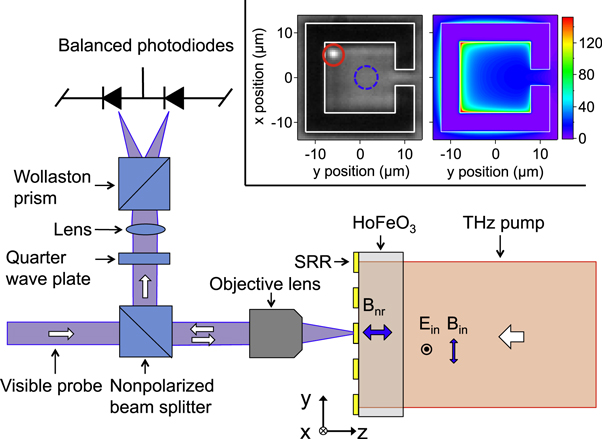
Figure 1. Schematic setup of THz pump-visible MOKE measurement. The left side of the inset shows the photograph of SRR fabricated on the c-cut surface of the HoFeO3 crystal and the white solid line indicates the edge of the SRR. The red solid and blue dashed circles indicate the probe spots for the MOKE measurement. The right side of the inset shows the spatial distribution of the enhancement factor calculated by the FDTD method, i.e., the ratio between the Fourier amplitude at νLC of the z-component of Bnr (at z = 0) and the incident THz pulse Bin.
Download figure:
Standard image High-resolution imageAt room temperature, the two magnetizations mi (i = 1, 2) of the different iron sublattices in HoFeO3 are almost antiferromagnetically aligned along the x-axis with a slight canting angle β0(=0.63°) owing to the Dzyaloshinskii field and form a spontaneous magnetization MS along the z-axis [30]. In the THz region, there are two antiferromagnetic resonance modes (quasiantiferromagnetic (AF) and quasiferromagnetic (F) mode [31]). The magnetic field Bnr generated along the z-axis in our setup causes AF-mode motion; as illustrated in figure 2(a), the Zeeman torque pulls the spins along the y-axis, thereby triggering precessional motions of mi about the equilibrium directions. The precessional motions cause the macroscopic magnetization M = m1 + m2 to oscillate in the z-direction [32, 33]. The resultant magnetization change ΔMz(t) modulates the anti-symmetric off-diagonal element of the dielectric tensor  and induces a MOKE signal (Kerr ellipticity change Δθ) [34, 35] (see appendix
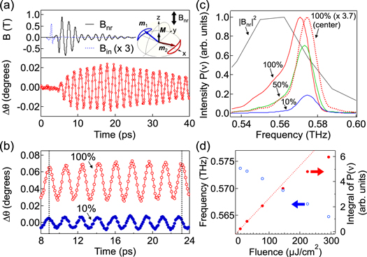
Figure 2. (a) Upper panel: incident magnetic field of the THz pump pulse Bin estimated by electro-optic sampling (dashed line) and the THz magnetic near-field Bnr calculated by the FDTD method (solid line). The illustration shows the magnetization motion for the AF-mode. Lower panel: the MOKE signal for a pump fluence of 292 μJ cm−2 (100%). (b) Comparison of two MOKE signals for different pump fluences, vertically offset for clarity. (c) The FFT power spectrum of the magnetic near-field Bnr (black solid line). The spectra P(ν) of the MOKE signals for a series of pump fluences obtained at the corner (solid lines) and at the center (blue dashed circle in the inset of figure 1) for a pump fluence of 100% (dashed line). Each spectrum of the MOKE signal is normalized by the peak amplitude at the corner for a pump fluence of 100%. (d) Intensity dependence of the center-of-mass frequency (open circles) and the integral (closed circles) of the P(ν).
Download figure:
Standard image High-resolution image3. Results and discussions
Figure 2(a) (upper panel) shows the calculated temporal magnetic waveform together with the incident magnetic field. The maximum peak amplitude is four times that of the incident THz pulse in the time domain and reaches 0.91 T. The magnetic field continues to ring until around 25 ps after the incident pulse has decayed away. The spectrum of the pulse shown in figure 2(c) has a peak at the LC resonance frequency (νLC = 0.56 THz) of the SRR, which is designed to coincide with the resonance frequency of the AF-mode ( Figure 2(a) (lower panel) shows the time development of the MOKE signal Δθ for the highest THz excitation intensity (pump fluence I of 292 μJ cm−2 and maximum peak magnetic field Bmax of 0.91 T). The temporal evolution of Δθ is similar to that of the Faraday rotation measured in the previous study and the magnetization oscillates harmonically with a period of ∼2 ps [23], implying that the THz magnetic field coherently drives the AF-mode motion.
As shown in figure 2(b), as the incident pump pulse intensity increases, the oscillation period becomes longer. The Fourier transform spectra of the MOKE signals for different pump intensities are plotted in figure 2(c). As the excitation intensity increases, the spectrum becomes asymmetrically broadened on the lower frequency side and its peak frequency becomes redshifted. Figure 2(d) plots the center-of-mass frequency (open circles) and the integral (closed circles) of the power spectrum P(ν) as a function of incident pulse fluence. The center frequency monotonically redshifts and P(ν) begins to saturate. As shown in figure 2(c), the MOKE spectra obtained at the center of the SRR (indicated in the inset of figure 1) does not show a redshift even for the highest intensity excitation, suggesting that the observed redshift originates from the nonlinearity of the precessional spin motion rather than that of the SRR response. We took the analytic signal approach (ASA) to obtain the time development of the instantaneous frequency ν(t) (figure 3(c)) and the envelope amplitude ζ0(t) (figure 3(d)) from the measured magnetization change ζ(t) = ΔMz(t)/|MS| (figure 3(b)) (see appendix  This result indicates that the signals below t = 25 ps are affected by the persisting driving field and the redshift may originate from the forced oscillation. As long as the magnetic response is under the linear regime, the instantaneous frequency is independent on the pump fluence. However, for the high pump fluence (100%) a redshift (a maximum redshift of ∼15 GHz relative to the constant frequency
  appears in the delay time (t < 25 ps) and even after the driving field decays away (t > 25 ps) the frequency continues to be redshifted as long as the amplitude of the magnetization change is large. These results suggest that the frequency redshift in the high intensity case depends on the magnitude of the magnetization change, implying that its origin is a nonlinear precessional spin motion with a large amplitude.

Figure 3. (a) FDTD calculated magnetic field Bnr for pump fluence of 100%. (b) Temporal evolution of the magnetization change obtained from the experimental data (gray circles) and the LLG model (red line). (c) Instantaneous frequencies and (d) envelope amplitudes for pump fluences of 100% and 10% obtained by the analytic signals calculated from the experimental data (circles) and the LLG simulation with nonlinear damping parameter (α1 = 1 × 10⁻³, solid lines) and without one (α1 = 0, dashed line).
Download figure:
Standard image High-resolution imageThe temperature increase due to the THz absorption (for HoFeO3 ΔT = 1.7 × 10⁻³ K, for gold SRR ΔT = 1 K) is very small (see appendix
Figure 4 shows a parametric plot of the instantaneous frequency ν(t) and envelope amplitude ζ0(t) for the high pump fluence (100%). The instantaneous frequency shift for t > 25 ps has a square dependence on the amplitude, i.e.,  To quantify the relationship between the redshift and magnetization change, it would be helpful to have an analytical expression of the AF mode frequency νAF as a function of the magnetization change, which is derived from the LLG equation based on the two-lattice model [32, 33]. The dynamics of the sublattice magnetizations mi (i = 1, 2), as shown in the inset of figure 2(a), are described by

where Ri = mi/m0 (m0 = |mi|) is the unit directional vector of the sublattice magnetizations, γ = 1.76 × 10¹¹ s−1 T−1 is the gyromagnetic ratio, V(Ri) is the free energy of the iron spin system normalized with m0, and  is the effective magnetic field given by
  (i = 1, 2) (see appendix
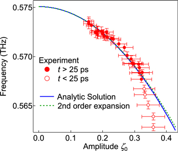
Figure 4. Relation between instantaneous frequency ν and envelope amplitude ζ0 obtained from the magnetization change; for t < 25 ps (open circles) and for t > 25 ps (closed circles), the analytic solution (blue line) and second order expansion of the analytic solution (green dashed line). Errors are estimated from the spatial inhomogeneity of the driving magnetic field (see appendix
Download figure:
Standard image High-resolution imageSince Beff, i depends on the sublattice magnetizations mi and the product of these quantities appears on the right side of equation (1), the LLG equation is intrinsically nonlinear. If the angle of the sublattice magnetization precession is sufficiently small, equation (1) can be linearized and the two fixed AF- and F-modes for the weak excitation can be derived. However, as shown in figure 3(b), the deduced maximum magnetization change ζ reaches ∼0.4, corresponding to precession angles of 0.25° in the xz-plane and 15° in the xy-plane. Thus, the magnetization change might be too large to use the linear approximation. For such a large magnetization motion, assuming the amplitude of the F-mode is zero and α = 0 in equation (1), the AF mode frequency νAF in the nonlinear regime can be deduced as


where K(D) is the complete elliptic integral of the first kind, rAF( 60) is the ellipticity of the sublattice magnetization precession trajectory of the AF-mode (see appendix
  and matches the observed redshift for t > 25 ps, showing that the frequency approximately decreases with the square of ζ(t). The discrepancy of the experimental data from the theoretical curve (t < 25 ps) may be due to the forced oscillation of the AF-mode caused by the driving field.
To elaborate the nonlinear damping effects, we compared the measured ζ(t) with that calculated from the LLG equation with the damping term. As shown in figures 3(c) and (d), the experiment for the high intensity excitation deviates from the simulation with a constant Gilbert damping (dashed lines) even in the t > 25 ps time region, suggesting nonlinear damping becomes significant in the large amplitude region. To describe the nonlinear damping phenomenologically, we modified the LLG equation so as to make the Gilbert damping parameter depend on the displacement of the sublattice magnetization from its equilibrium position, α(Ri) = α0 + α1ΔRi. As shown in figures 3(b)–(d), the magnetization change ζ(t) derived with equation (1) (solid line) with the damping parameters (α0 = 2.27 × 10⁻⁴ and α1 = 1 × 10⁻³) nicely reproduces the experiments for both the high (100%) and low (10%) excitations6 . These results suggest that the nonlinear damping plays a significant role in the large amplitude magnetization dynamics. Most plausible mechanism for the nonlinear damping is four magnon scattering process, which has been introduced to quantitatively evaluate the magnon mode instability of ferromagnet in the nonlinear response regime [37].
4. Conclusions
In conclusion, we studied the nonlinear magnetization dynamics of a HoFeO3 crystal excited by a THz magnetic field and measured by MOKE microscopy. The intense THz field can induce the large magnetization change (∼40%), and the magnetization change can be kept large enough to induce the redshift even after the field has gone, enabling us to separate the contributions of the applied magnetic field and magnetization change to the frequency shift in the time domain. The resonance frequency decreases in proportion to the square of the magnetization change. A modified LLG equation with a phenomenological nonlinear damping term quantitatively reproduced the nonlinear dynamics. This suggests that a nonlinear spin relaxation process should take place in a strongly driven regime. This study opens the way to the study of the practical limits of the speed and efficiency of magnetization reversal, which is of vital importance for magnetic recording and information processing technologies.
Acknowledgments
We are grateful to Shintaro Takayoshi, Masahiro Sato, and Takashi Oka for their discussions with us. This study was supported by a JSPS grants (KAKENHI 26286061 and 26247052) and Industry-Academia Collaborative R&D grant from the Japan Science and Technology Agency (JST).
Appendix A.: Detection scheme of MOKE measurement
We show the details of the detection scheme of the MOKE measurement. A probe pulse for the MOKE measurement propagates along the z-direction. By using the Jones vector [38], an electric field E0 of the probe pulse polarized linearly along the x-axis is described as

The probe pulse E1 reflected from the HoFeO3 surface becomes elliptically polarized with a polarization rotation angle ϕ and a ellipticity angle θ. It can be written as

where  is the Jones matrix describing π/2 phase retardation of the y component with respect to the x component

and  is the rotation matrix

The reflected light passes through the quarter wave plate, which is arranged such that its fast axis is tilted by an angle of 45° to the x-axis. The Jones matrix of the wave plate is given by

Thus, the probe light E2 after the quarter wave plate is described as follows

The Wollaston prism after the quarter wave plate splits the x and y-polarization components of the probe light E2. The spatially separated two pulses are incident to the balanced detector and the detected probe pulse intensity ratio of the differential signal to the total corresponds to the Kerr ellipticity angle as follows

In the main text, we show the Kerr ellipticity change Δθ = θw − θwo, where the ellipticity angles (θw and θwo) are respectively obtained with and without the THz pump excitation.
Appendix B.: ASA and short time Fourier transform (STFT)
The ASA allows the extraction of the time evolution of the frequency and amplitude by a simple procedure and assumes that the signal contains a single oscillator component. In our study, we measure only the MOKE signal originating from the AF-mode and it can be expected that the single oscillator assumption is valid. In the ASA, the time profile of the magnetization change ζ(t) is converted into an analytic signal ψ(t), which is a complex function defined by using the Hilbert transform [39]


where the p is the Cauthy principal value. The real part of ψ(t) corresponds to ζ(t). The real function ζ0(t) and ϕ(t) represent the envelope amplitude and instantaneous phase of the magnetization change. The instantaneous frequency ω(t)(=2πν(t)) is given by ω(t) = dϕ(t)/dt. In the analysis, we averaged ζ0(t) and ω(t) over a ten picosecond time range.
To confirm whether the ASA gives appropriate results, as shown in figure B.1 we compare them with those obtained by the STFT. As shown in figure B.1(a), the time–frequency plot shows only one oscillatory component of the AF-mode. As shown in figures B.1(b) and (c), the instantaneous frequencies and amplitudes obtained by the ASA and the STFT are very similar. Because the ASA provides us the instantaneous amplitude with a simple procedure, we showed the time evolutions of frequency and amplitude derived by the ASA in the main text.

Figure B.1. (a) Time-dependence of the power spectrum of the magnetization oscillation for the highest THz excitation (I = 292 μJ cm−2) obtained by the STFT. Comparison of (b) instantaneous frequencies and (c) amplitudes obtained by the ASA and STFT with a time window with FWHM of 10 ps.
Download figure:
Standard image High-resolution imageAppendix C.: Determination of conversion coefficient g and linear damping parameter α0
The conversion coefficient g and the linear damping parameter α0(=α) in equation (1) are determined by fitting the experimental MOKE signal Δθ(t) for the low pump fluence of 29.2 μJ cm−2 with the LLG calculation of the magnetization change ζ(t). Figure C.1 shows the MOKE signal Δθ(t) (circle) and the calculated magnetization change ζ(t) (solid line). From the least-squares fit of the calculated result to the experiment by using a linear relation, i.e., ζ(t) = gΔθ(t), we obtained the parameters g(=17.8 degrees−1) and α0(=2.27 × 10⁻⁴).

Figure C.1. Experimentally observed MOKE signal Δθ (circle) and LLG simulation result of the magnetization change ζ (solid line) for the pump fluence of 29.2 μJ cm−2.
Download figure:
Standard image High-resolution imageAppendix D.: Laser heating effect
The details of the calculation of the temperature change are as follows:
- For HoFeO3:
The absorption coefficient αabs of HoFeO3 at 0.5 THz is ∼4.4 cm−1 [40]; the fluence IHFO absorbed by HoFeO3 can be calculated as IHFO = I(1−exp(−αabsd)), where d (=145 μm) is the sample thickness and I is the THz pump fluence. For the highest pump fluence, I = 292 μJ cm−2, IHFO is 18.1 μJ cm−2. Since the sample thickness is much smaller than the penetration depth,  we assume that the heating of the sample due to the THz absorption is homogeneous. By using the heat capacity Cp of 100 J mol−1 K−1 [27], and the molar volume v of ∼1.4 × 102 cm3 mol−1 [27], the temperature change ΔT can be estimated as ΔT = IHFOv/Cpd ∼ 1.7 × 10⁻³ K.
- For gold resonator (SRR):
The SRR has an absorption band (center frequency ∼0.56 THz, band width ∼50 GHz) originated from the LC resonance (figure 2(c)). Assuming the SRR absorbs all incident THz light in this frequency band, the absorbed energy accounts for 3% of the total pulse energy. Hence, for the highest THz pump fluence, I = 292 μJ cm−2, the fluence absorbed by the SRR is Igold = 8.76 μJ cm−2. By using the heat capacity Cp of 0.13 J g−1 K−1 [41], the number of the SRRs per unit area N of 4 × 104 cm−2, and the mass of the SRR m of 1.6 × 10⁻⁹ g, the temperature change ΔT can be estimated as ΔT = Igold/CpNm ∼ 1 K.
Appendix E.: Free energy of HoFeO3
The free energy F of the iron spin (Fe3+) system based on the two-lattice model is a function of two different iron sublattice magnetizations mi, and composed of the exchange energy and one-site anisotropy energy [32, 33]. The free energy normalized by the sublattice magnetization magnitude, V = F/m0 (m0 = |mi|), can be expanded as a power series in the unit directional vector of the sublattice magnetizations, Ri = mi/m0 = (Xi, Yi, Zi). In the magnetic phase Γ4 (T > 58 K), the normalized free energy is given as follows [32, 33]:

where E(=6.4 × 10² T) and D(=1.5 × 10 T) for HoFeO3 are respectively the symmetric and antisymmetric exchange field [42]. Axx and Azz are the anisotropy constants. As mentioned in appendix F, the temperature dependent values of the anisotropy constants can be determined from the antiferromagnetic resonance frequencies. The canting angle of Ri to the x-axis  under no magnetic field is given by

Appendix F.: Linearized resonance modes and anisotropy constants (Axx and Azz)
The nonlinear LLG equation of equation (1) can be linearized and the two derived eigenmodes correspond to the AF and F-mode. The sublattice magnetization motion for each mode is given by the harmonic oscillation of mode coordinates; for the AF-mode (QAF, PAF) = ((X1 − X2) + (Z1 + Z2)
 Y1 − Y2), and for the F-mode (QF, PF) = ((X1 + X2)
 − (Z1−Z2)
 Y1 + Y2),


where AAF,F represents the amplitude of each mode. ωAF,F, and rAF,F are the resonance frequencies and ellipticities, which are given by


where γ = 1.76 × 10¹¹ s−1 T−1 is the gyromagnetic ratio, and


Substituting the literature values of the exchange fields (E = 6.4 × 10² T and D = 1.5 × 10 T [42]) and the resonance frequencies at room temperature (ωAF/2π = 0.575 THz and ωF/2π = 0.37 THz) to equations (F.5) and (F.6), Axx and Azz can be determined to 8.8 × 10⁻² T and 1.9 × 10⁻² T.
Appendix G.: MOKE measurement for the spontaneous magnetization
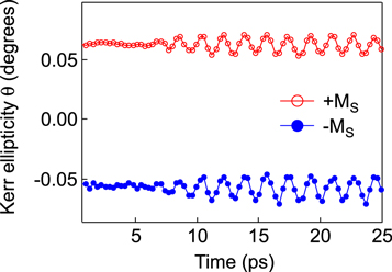
Figure G.1. The MOKE signals, the temporal change of the Kerr ellipticity  measured for different initial conditions with oppositely directed magnetizations.
Download figure:
Standard image High-resolution imageFigure G.1 shows time-development of the MOKE signals for the different initial condition with oppositely directed magnetization. We applied the static magnetic field (∼0.3 T) to saturate the magnetization along the z-axis before the THz excitation. The spontaneous magnetization of single crystal HoFeOa can be reversed by the much smaller magnetic field (∼0.01 T) because of the domain wall motion [27]. Then, we separately measured the static Kerr ellipticity angle θoffset and THz induced ellipticity change Δθ for different initial magnetization Mz = ±Ms without the static magnetic field. In figure G.1 we plot the summation of the time resolved MOKE signal Δθ and the static Kerr ellipticity θoffset. The sings of the ellipticity offset angle θoffset for the different spontaneous magnetization (±MS) are different and their magnitudes are ∼0.05 degrees. The conversion coefficient g(=1/θ ∼ 1/0.05 degrees) is estimated to be ∼20 degrees−1, which is similar to the value determined by the LLG fitting (∼17.8 degrees−1). In the case of the AF-mode excitation, the phases of the magnetization oscillations are in-phase regardless of the direction of the spontaneous magnetization M = ±Ms, whereas they are out-of-phase in the case of the F-mode excitation. We can explain this claim as follows: in the case of AF-mode excitation, the external THz magnetic field is directed along the z-direction as shown in the inset of figure 2(a), the signs of the torques acting on the sublattice magnetization mi (i = 1, 2) depends on the direction of mi, however, the resultant oscillation of the macroscopic magnetization M = m1 + m2 along the z-direction has same phase for the different initial condition M = ±Ms. In the case of the F-mode excitation with the external THz magnetic field along the x- or y-direction, the direction of the torques acting on the magnetization M depends on the initial direction and the phase of the F-mode oscillation changes depending on the sign of the spontaneous magnetization ±Ms.
Appendix H.: Influence of the spatial distribution of magnetic field on magnetization change
As shown in the inset of figure 1, the pump magnetic field strongly localizes near the metallic arm of the SRR and the magnetic field strength significantly depends on the spatial position r within the probe pulse spot area. The intensity distribution of the probe pulse Iprobe(r) has an elongated Gaussian distribution with spatial widths of 1.1 μm along the x-axis and 1.4 μm along the y-axis (full width at half maximum (FWHM) intensity). The maximum magnetic field is 1.2 times larger than the minimum one in the spot diameter, causing the different magnetization change dynamics at different positions. To take into account this spatial inhomogeneity to the simulation, the spatially weighted average of magnetization change  has to be calculated as follows:

where ζ(r, t) is a magnetization change at a position r and time t.
Figure H.1(a) shows the simulation result of the spatially averaged magnetization change  and the non-averaged ζ(r0, t) without the nonlinear damping term (α1 = 0), where r0 denotes the peak position of Iprobe(r). For the low excitation intensity (10%),
  is almost the same as ζ(r0,t) as shown in figure H.1(a). On the other hand, for the high excitation intensity, the spatial inhomogeneity of magnetization change dynamics induces a discrepancy between the
  and ζ(r0,t). This discrepancy is caused by the quasi-interference effect between the magnetization dynamics with different frequencies and amplitudes at different positions. Figures H.1(b) and (c) show the instantaneous frequency and envelope amplitude obtained from the data shown in figure H.1(a) by using ASA with the experimental result. For the averaged magnetization change, the frequency redshift is more emphasized (figure H.1(b)) and the decay time becomes shorter (figure H.1(c)). Nonetheless, neither spatially averaged nor non-averaged simulation reproduces the experimental result of the instantaneous frequency (figure H.1(b)) without nonlinear damping term.

Figure H.1. Comparison of the spatially averaged and non-averaged magnetization change for the different pump fluences of 10% and 100%. (a) Temporal evolutions of the magnetization change, (b) instantaneous frequencies and (c) normalized envelope amplitudes. Open circles show the experimental results.
Download figure:
Standard image High-resolution image
Footnotes
- 6
The damping parameter α0 (=2.27 × 10⁻⁴) and conversion coefficient g (=17.8 degrees−1) are determined from the least-squares fit of the calculated result without the nonlinear damping parameter α1 to the experimental MOKE signal for the low pump fluence of 29.2 μJ cm−2. The nonlinear damping parameter α1 (=1.0 × 10⁻³) is obtained by fitting the experimental result for the high intensity case (I = 292 μJ cm−2) with the values of α0 and g obtained for the low excitation experiment. The estimated value of g is consistent with the static MOKE measurement; the Kerr ellipticity induced by the spontaneous magnetization MS is ∼0.05 degrees (g ∼ 20 degrees−1). See appendix G for details on the static Kerr measurement.