


Abstract
We extend time-domain imaging in acoustic metamaterials to gigahertz frequencies. Using a sample consisting of a regular array of ∼1 μm diameter silica microspheres forming a two-dimensional triangular lattice on a substrate, we implement an ultrafast technique to probe surface acoustic wave propagation inside the metamaterial area and incident on the metamaterial from a region containing no microspheres, which reveals the acoustic metamaterial dispersion, the presence of band gaps and the acoustic transmission properties of the interface. A theoretical model of this locally resonant metamaterial based on normal and shear-rotational resonances of the spheres fits the data well. Using this model, we show analytically how the sphere elastic coupling parameters influence the gap widths.
Export citation and abstract BibTeX RIS

Original content from this work may be used under the terms of the Creative Commons Attribution 3.0 licence. Any further distribution of this work must maintain attribution to the author(s) and the title of the work, journal citation and DOI.
Introduction
Wave propagation in metamaterials has led to a host of new perspectives in wave control owing to their tailorable properties. These effective properties include the permittivity and permeability in the electromagnetic case [1, 2], and the density and elastic modulus in the acoustic case [3–5]. Applications that have been explored as a result of this tailorability include cloaking when the parameters are spatially varied [6–8], wave damping when there is a single negative parameter [3, 4, 9, 10], and near-field super-resolution when either one or both parameters are negative [10–14]. Owing to the resulting complex, spatiotemporally varying wave fields, time-domain imaging in metamaterials is thus crucially important to their understanding.
Although time-domain imaging of acoustic waves in metamaterials has been carried out in a variety of studies [15–19], to date the frequency range has been restricted to below 1 MHz. Building on progress in imaging surface acoustic waves (SAWs) in phononic crystals [20–24], in this paper we present results for time-domain imaging of gigahertz-frequency SAWs on a regular array of silica microspheres adhered to a substrate—an acoustic metamaterial exhibiting contact resonances [25–28]—using ultrashort optical point-source excitation inside and outside the metamaterial region. By means of Fourier transforms we derive the acoustic dispersion relation and probe the transmission properties at different frequencies, and interpret the results with an analytical model of the microsphere resonant interactions between themselves and with the substrate.
The sample is similar to that studied by Boechler et al [26], consisting of a monolayer of silica microspheres, hereafter referred to as beads, of diameter  and density
  on a 1.5 mm thick float-glass substrate, as shown in figure 1(a). The glass substrate is coated with a 100 nm thick aluminium film in order to facilitate excitation of acoustic waves. The bead layer is then assembled on the substrate using the wedge-shaped cell convective self-assembly technique, in a manner similar to [26]. At short range, the beads form a triangular lattice; however, multiple defects and grain boundaries are present within the measurement area, as is shown in the optical image of the monolayer in figure 1(b).
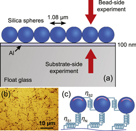
Figure 1. (a) Diagram of the cross section of the sample, showing a monolayer of 1.08 μm diameter spheres on a glass substrate with a thin Al film coating. The red arrows represent the directions of incidence of the laser beams for the bead-side and substrate-side experiments. (b) Optical image of the sample surface. (c) Schematic diagram representing a theoretical model consisting of spheres connected by massless springs. The normal, shear bead-surface, and shear bead-bead stiffness constants are  ,
,  and
and  , respectively.
Download figure:
Standard image High-resolution imageResults
Experimental
We use a time-resolved two-dimensional SAW imaging technique based on an optical pump-probe system operating at a repetition rate of ∼80 MHz [29]. We perform two types of experiment. In the first type, we probe the bead side of the sample in order to obtain contributions to the detected signals from the beads and to allow direct comparisons between acoustic and optical images. In the second type, we probe from the substrate side of the sample in order to avoid any effects of the interaction of the beads with the probe light. The use of spatiotemporal Fourier transforms allows access to frequency-resolved data down to 6 MHz resolution.
The light source is a mode-locked Ti-sapphire laser generating light pulses of central wavelength 830 nm and pulse duration ∼100 fs at a repetition rate of ∼80 MHz. Frequency-doubled 415 nm light pulses are used for the pump, and 830 nm light pulses are used for the probe, with spot diameters ∼2 μm and respective pulse energies 0.1 and 0.05 nJ. The probe spot size is sufficient to resolve spatial details commensurate with the bead diameter. After passing through an acousto-optic modulator that chops the pump beam, the pump pulses thermoelastically excite acoustic waves up to ∼1 GHz with surface displacements ∼10 pm. The continuous repetition of the pump pulses induces a nondestructive local transient temperature rise of ∼50 K and steady-state temperature rise of ∼15 K. The probe beam passes through a common-path interferometer [29], which produces a photodetector output proportional to the component of the acoustic particle velocity normal to the sample surface. For the lower frequency resolution experiments this output is fed to a lock-in amplifier, which synchronously records the in-phase component at the chopping frequency as a function of the probe spot position, which is scanned relative to the pump. This configuration allows an acoustic frequency resolution of ∼80 MHz. For the experiments with higher frequency resolution, we make use of an intensity-modulation scheme for both the pump and probe beams [30]. A delay line is installed in the probe light path, and an extra acousto-optic modulator is set upstream of the delay line. For these experiments both the in-phase and quadrature components at the lock-in amplifier are monitored. This configuration allows fine control of the detected acoustic frequency to ∼25 MHz resolution.
Bead-side imaging
We first image on the bead side, selecting a region near the border between the bead-free surface and the metamaterial region containing the beads. With the position of the pump spot fixed, the probe spot position is focused on the substrate surface and scanned across a  area. The delay time between the pump and the probe pulses is varied from 0 to 12.4 ns, corresponding to the laser repetition rate of 80.4 MHz, and 35 images are recorded at regular time intervals. In these experiments, the pump beam is chopped at a frequency of 1.1 MHz for lock-in detection.
Figure 2(a) shows a probe-beam reflectivity image of the selected region, where the darker section is a metamaterial region and the remainder is a bead-free region. The figure demonstrates an imaging resolution sufficient to discern defects and grain boundaries (c.f. figure 1(b)). We focused the pump to a point on the bead-free surface, as indicated by the central red spot in figure 2(a). Figure 2(b) shows an image over the same area of the normal surface particle velocity at the moment of the pump pulse arrival. The solid black lines indicate the border between the bead-free and metamaterial regions. A circular Rayleigh-wave (RW) wavefront can be seen propagating from the excitation point arising from the pump pulse prior to the one arriving the centre of the image, yielding a surface-wave velocity of  , of the same order as that previously observed for similar float-glass substrates [26, 28, 31]. There are most likely contributions to the signal from both interface and bead motion, although we cannot differentiate between the two. In spite of the interaction of the probe light with the beads, we are still able to clearly resolve the acoustic wavefronts in the metamaterial region, which appear with reduced amplitude. In the time domain, however, the influence of the metamaterial on the SAW velocity is not immediately apparent. The measured velocity corresponds closely to that of the RW on float glass,
  , calculated using Young's modulus
  , Poisson's ratio
  and density
  [32]. The longitudinal and transverse acoustic velocities of float glass are
  and
and  , respectively.
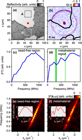
Figure 2. Experimental results for bead-side imaging. (a) Optical probe-beam reflectivity image of the scanned region. The darker area corresponds to the metamaterial region and the lighter area corresponds to the bead-free region. Red dot: location of pump spot. Dotted boxes A and B: regions sampled for the spectra shown in the insets of (e) and (f), respectively. (b) Snapshot of the acoustic field ( , where
  is the position vector and t is the time) at
  , showing the propagating SAW wavefront resulting from the previous laser pulse. The solid black outline shows the border of the metamaterial region. (c) Frequency spectrum corresponding to the bead-free region obtained from the averaged modulus of the temporal Fourier transform (
 ). (d) Frequency spectrum corresponding to the metamaterial region, showing two dips in amplitude around 320 and 640 MHz. The vertical bar and thin line indicate band gaps obtained by theoretical analysis and fits to experimental data for both bead-side and substrate-side imaging. (e) Modulus of the spatiotemporal Fourier transform
  of the acoustic field in the bead-free region A, representing the dispersion relation for + y-directed propagation. The inset shows a straight-line cross section obtained from the bright region of the image. (f) Modulus of the spatiotemporal Fourier transform of the acoustic field in the metamaterial region B, representing the dispersion relation for −y-directed propagation. The inset shows a straight-line cross section obtained from the bright region of the image, with the horizontal axes reversed for ease of comparison with the inset of (e).
Download figure:
Standard image High-resolution imageFigure 2(c) shows the acoustic frequency spectrum corresponding to the bead-free surface, obtained from the average modulus of temporal Fourier transforms sampled over the entire bead-free region (i.e. the regions outside the black lines in figure 2(b)), indicating a broad response up to frequencies >1 GHz. Figure 2(d) shows the equivalent frequency spectrum for the metamaterial region, sampled over the entire metamaterial region (i.e. inside the black lines). The general trend is similar, but two dips appear at around 320 and 640 MHz. As discussed below, this attenuation arises in the region of gaps in the dispersion relation, and can be explained by hybridization of the propagating RWs with the vibrational resonances of the beads interacting between themselves and with the surface [26–28]. Such resonant attenuation has been previously accounted for using a damped oscillation model of the bead dynamics [31]. In contrast to the previous study [26], we record a larger resonant frequency by a factor of ∼1.5 associated with bead vibrations normal to the surface. Variations in the contact resonance frequency have previously been observed and hypothesized to be caused to factors that stem from variations in the sample preparation procedure [33]. In addition, the formation of solid bridges near the contact due to impurities in the colloidal solution and capillary effects have also been suggested as a possible cause of stiffer contacts [34].
Constant-frequency images of the real part of the temporal Fourier transform at intervals of the laser repetition rate, i.e. 80.4 MHz, are shown in figure 3(a) for various frequencies. At 241 MHz, the circular ripple pattern is fairly uniform over the surface, although it is weaker in the metamaterial regions owing to the lower optical reflectivity (0.85). At 321 MHz, the transmission to the metamaterial region is very small. At 482 MHz, the ripple pattern is again fairly uniform, but weaker in the metamaterial regions owing to a combination of lower optical reflectivity and lower transmission. At 643 MHz, there is again a marked difference in wave amplitude between the metamaterial and the bead-free regions, as was the case at 321 MHz. The behaviour at 321 MHz and 643 MHz is consistent with the regions of extra attenuation noted above in the acoustic frequency spectrum of the metamaterial region (figure 2(d)). Figure 3(b) shows corresponding constant-frequency images in k-space, obtained from the modulus of the spatial Fourier transform of the data in figure 3(a) in each case, showing that the surface waves have the highest amplitude in the direction away from the upper boundary between the metamaterial and the bead-free surface owing to the dominant contribution from the +y-excited waves on the bead-free surface. The circular rings in each case confirm the isotropic nature of the dispersion relations. Figures 2(e) and (f) represent the dispersion relations in the bead-free and metamaterial regions, respectively, obtained from the modulus of spatiotemporal Fourier transforms in regions A and B in figure 2(a) for y-directed propagation, illustrating clear amplitude dips for the metamaterial region at wave numbers corresponding to ∼320 MHz and ∼640 MHz, in agreement with the corresponding dips in figure 2(d). The smaller dip height in figure 2(d) is caused by the inclusion of all wave vectors in the averaging process (over the metamaterial that contains grain boundaries and defects) involved in producing the curve of figure 2(d). The overall dispersion of both the bead-free and metamaterial regions can be represented by an approximately straight line with a phase velocity around  , as previously mentioned. However, the experimental frequency resolution is not sufficient to observe the expected deviations in velocity for the metamaterial in the region of the gaps.

Figure 3. Frequency-resolved images of the real part (A cos ϕ) of the temporal Fourier transform of the acoustic field on the sample surface at selected frequencies. (a) Real space images. (b)  -space images of the modulus of the spatiotemporal Fourier transform
  evaluated over the whole imaged area.
Download figure:
Standard image High-resolution imageIn the next section we investigate the frequency response of the metamaterial in more detail using higher frequency resolution, and also make use of probing from the substrate side of the sample in order to provide a comparative set of data.
Substrate-side imaging
Imaging through the transparent substrate at the glass-aluminium interface avoids optical interaction between the probe light and the beads, thus simplifying the detection mechanism. Boechler et al [26] observed that for a sample with the same bead array as in the present experiments, measuring from the substrate side preferentially detects the interface motion, whereas measuring from the bead side preferentially detects the bead motion. So probing from the substrate side therefore provides complementary information on the metamaterial dynamics.
For these experiments, we also considerably improve the frequency resolution compared with the previous section by making use of an arbitrary-frequency set-up [30, 35]. The laser repetition frequency is set to  for these experiments. We record two space-time imaging scans, each of 41 frames covering a
  2 area with ∼25 MHz frequency resolution obtained by adjusting the pump and probe modulation frequencies.
Figure 4 shows an example of a snapshot of the acoustic propagation in a region completely covered with beads, obtained 7.7 ns after the arrival of a pump pulse. As in the bead-side images, the circular SAW wavefronts are evident. A notable difference here is that a faster surface-skimming longitudinal mode wavefront is also clearly visible, which is detected via refractive index changes in the glass. Such surface-skimming longitudinal mode wavefronts have previously been noted in similar samples [26, 31]. The surface-skimming longitudinal mode wavefront velocity is measured to be  , which agrees well with the value
  calculated from the literature [32].

Figure 4. Snapshot of the acoustic field ( )) 7.7 ns after the arrival of a pump pulse obtained by probing from the substrate side of the sample. SAW indicates a Rayleigh-like surface wave. SSLW indicates a surface-skimming longitudinal wave. In the corners of the image, the wavefront of a SAW excited in the previous laser cycle is visible.
Download figure:
Standard image High-resolution imageIn contrast to the simple pump-beam modulation system used for the bead-side imaging, the use of an arbitrary-frequency set-up requires the monitoring of the complex output signal X + iY of the lock-in amplifier. We process this output to obtain the spatiotemporal Fourier transform of X + iY to extract frequency-resolved images of its modulus in both real space and  -space [30, 35]. Figures 5(a)–(c) shows constant-frequency images at 226 MHz, 302 MHz and 378 MHz, which again reveal attenuated SAW propagation at ∼300 MHz compared with nearby frequencies. As before, a spatial Fourier transform of the constant-frequency data allows
  -space to be accessed. Figures 5(d)–(f) shows such images at the same frequencies, where the different modes can be identified by their respective propagation speeds. The large circles represent the slower Rayleigh-like SAWs, and the smaller circles represent the surface-skimming longitudinal waves (SSLWs). The more solid appearance of the rings compared with figure 3 is due to the prominence of the SSLWs, which have smaller
  at a given frequency. Examining the real- and
  -space images at 302 MHz in figure 5 indicates that the wave pattern at this frequency arises almost exclusively from the faster, longer-wavelength, SSLW waves, as expected because of the extra attenuation of the SAWs noted near this frequency.

Figure 5. Constant-frequency images for substrate-side probing. Left-hand side: real space images of the real part (A cos ϕ) of the temporal Fourier transform. Right-hand side:  -space images of the modulus of the spatiotemporal Fourier transform
  evaluated over the whole imaged area.
Download figure:
Standard image High-resolution imageOver the ∼100 μm range of the experimental images, anisotropy of the Fourier modulus in  -space is not apparent, and circular features are formed, as was the case for the bead-side imaging, although some deviations from isotropic behavior are apparent owing to the presence of defects and grain boundaries. Our use of directional averages in polar coordinates
  in
in  -space to extract the acoustic dispersion relation mitigates this effect.
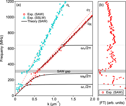
Figure 6(a) shows the experimental dispersion relation obtained by finding the  values corresponding to the peak Fourier modulus at each frequency up to 1.2 GHz after directional averaging. The red circles represent the SAW branch, whereas the blue triangles represent the SSLW branch. The dashed lines correspond to Rayleigh (cR), transverse (cT) and longitudinal waves (cL) in the glass substrate. In the regions outside the bead-motion resonances, the measured dispersions for the SAW and SSLW branches agree very well with velocities cR and cL, respectively. It is not clear at present why the SSLW branch becomes undetectable below ∼300 MHz, at least as far as ∼150 MHz. Figure 6(b) shows the corresponding temporal Fourier transform modulus as a function of frequency for the SAW branch, revealing a dip at ∼300 MHz associated with the previously identified gap near this frequency. There may also be a slight dip at ∼600 MHz suggesting the presence of the second gap, also in agreement with the indications of bead-side imaging, although in this case the dip is not as clear as those in figures 2(d) and (f). The dip may be less apparent for these measurements owing to a combination of (i) different measurement locations and (ii) different measurement and signal processing approaches. For instance, small differences in the level of disorder, whether caused by disorder in the contact stiffnesses or in the interparticle contact network, between the two measurement locations may result in a less pronounced gap for the location corresponding to figure 6 owing to inhomogeneous broadening. Effects such as differences in the contact network would particularly affect the higher gap, as it is dependent upon interparticle contacts even at long wavelengths, whereas the lower gap, which we attribute to out-of-plane motion of the spheres, is not [27]. Along these lines, we note that this effect could be further exacerbated by the use of directional averaging, which was used in the analysis of figure 6. In order to elucidate these findings theoretically, we analyse our results on the basis of an analytical model in the next section.
Figure 6. (a) Experimental and theoretical dispersion relations. Black lines: SAW branches (theoretical). Red circles: SAW branch (experimental). Blue triangles: SSLW branch (experimental). Dashed lines: dispersion relations corresponding to dispersionless Rayleigh (cR), transverse (cT) and longitudinal waves (cL) in the glass substrate. Grey shading: theoretical gaps in the SAW branch. (b) Experimental normalized temporal Fourier transform modulus ( ) as a function of frequency, corresponding to the SAW branch in (a).
Download figure:
Standard image High-resolution image
Discussion
Surface metamaterials consisting of arrays of beads can be understood by means of theoretical models based on the interaction of the beads with the propagating SAWs, as well as interactions between bead nearest neighbours [26–28]. Our approach is similar to previous studies, involving the bead–surface normal interaction as well as the bead–surface shear and bead–bead shear interactions [36]. Internal vibrations of the beads themselves have frequencies higher than the lowest spheroidal resonance of the microspheres at  [26], and so are not relevant in our studied frequency range. Shear forces are non-central, and can induce rotations of the beads in addition to their translations. The beads are modelled as spheres that interact with the surface and each other through massless springs, as illustrated in figure 1(c). The stiffnesses corresponding to the different modes of interaction are
  ,
,  and
and  , respectively, for normal, shear bead–surface, and shear bead–bead interactions. Together the different interactions modify the forces on the coated-substrate surface. The following equation then governs the angular frequency ω as a function of wave number k in the approximation of a dispersionless, lossless substrate:
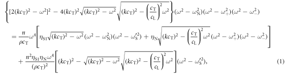
where cT and cL are the transverse and longitudinal substrate acoustic velocities, respectively, ρ is the substrate density and n is the surface concentration of beads (where  assuming hexagonal close packing). Here,
  is the resonance angular frequency corresponding to motion of the beads normal to the surface, and
  and
and  are those depending on shear interactions:


The quantities  ,
,  ,
,  and I are given by


where m is the bead mass. In the above derivation we have neglected the acoustic dispersion arising from the 100 nm aluminium film, which we regard as an excellent approximation [37]. The derivation of equation (1) closely follows the derivation, assumptions and approximations used to derive equation (14) in [27], not for a square- but for a hexagonal-lattice monolayer of beads [25]. As a consequence equation (1) is equivalent in its form to the equation that could have been obtained by equating the determinant of the matrix on the left-hand side of equation (14) from [27] to zero. The difference is in the relations between the total forces/moments acting on an individual bead from its neighbours and in the effective monolayer rigidities of the inter-bead contacts that emerge from the difference in the coordination number of the beads and their mutual orientation in the hexagonal and rectangular lattices.
Equation (1) can be solved for frequency in terms of wave vector ( ) or for wave vector in terms of frequency (
 ). Solving for wave vector as a function of frequency is pertinent to our case where constant-frequency imaging is available, and allows either real or complex wave vector solutions [38–43]. The imaginary part of a complex wave vector represents attenuation in the direction of propagation. In equation (1), pure real solutions correspond to SAW (Rayleigh-like) hybridization with bead resonances, similar to that observed previously [26]. Pure RWs on a uniform half-space do not exhibit dispersion, but at frequencies near the bead resonances the above model predicts a hybridization of these resonances with the SAWs. Fitting our data in figure 6(a) with the parameters
  ,
,  and
and  , we obtain the fit given by the solid black lines using parameters
  ,
,  and
and  kN m−1 and with corresponding resonance frequencies
  /2π = 292,
  /2π = 146 and
  /2π = 643 MHz. For the material properties we used the values given above. This fit is also chosen to be consistent with the bead-side data. The branches representing undamped waves exist in regions in which
  .
.
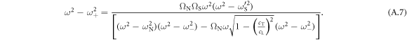
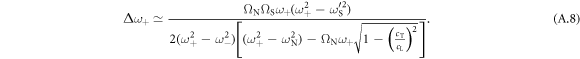
There is a gap associated with the  /2
/2  resonance of predicted width 38 MHz, indicated by the grey shading in figure 6(a), which corresponds to the dip in amplitude close to this frequency in both the bead- and substrate-side experiments (see figures 2(d) and 6(b), respectively). The lower boundary of this main gap is predicted to coincide with the resonance frequency of the normal vibrations of the bead relative to the surface. The upper boundary of this gap corresponds to the intersection of the modified Rayleigh mode (i.e. repelled by the resonance) with the bulk-shear acoustic wave branch. Below this frequency the modified Rayleigh mode becomes supersonic relative to the bulk-shear waves, and is attenuated by their emission. An approximate analytic expression for the main gap width associated with bead motion normal to the surface can in fact be derived (see appendix):

where  , and we have assumed
  and
and  , valid in our case. This gives
 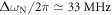 , in reasonable agreement with the numerically derived value of 38 MHz. A more accurate expression is given in the appendix.
A similar avoided-crossing effect is predicted above 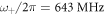 , the upper shear-rotational resonance, and gives rise to a smaller gap of width 0.38 MHz. This gap is also indicated by grey shading in figures 6(a) and (b). As with the main
  gap, the upper boundary corresponds to the intersection of the modified Rayleigh mode with the bulk-shear acoustic wave branch. The frequency 643 MHz of the model corresponds to the dip in amplitude near this frequency observed in the bead-side experiments, as shown in figure 2(d), although this is less clear in the substrate-side experiments, as shown in figure 6(b). A third resonance and avoided crossing are predicted above
 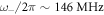 , the lower shear-rotational resonance. In this case, the 'gap' is negative, with a width of −1.60 MHz. This means that the modified Rayleigh branch above the resonance intersects the transverse (cT) branch at a lower frequency than the resonance frequency. This is likely to be caused by the dispersion relation of the horizontal resonance being modified by interaction with the SSLW branch so that it becomes slightly inclined in the vicinity of the cT branch.
Analytical expressions for the smaller gaps  and
and  can also be derived, as shown in detail in the appendix:
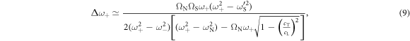
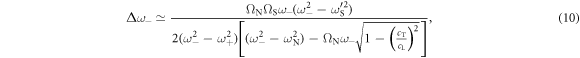
where  . In the above equations, the frequencies
  and
and  , being proportional to the surface concentration of beads and the spring rigidities, characterize the strength of the interactions. These values are relatively small compared with the resonance angular frequencies
  ,
,  and
and  . Equations (9) and (10) show that
  and
and  depend on
  , representing two interactions, whereas equation (8) shows that
  depends only on the larger value
  . This suggests that
  and
and  can be expected to be small compared with
  . Indeed, evaluation of equations (9) and (10) give values of
 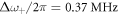 and
and 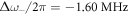 , respectively. These values agree well with the exact values of
 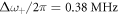 and
and 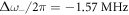 obtained directly by substituting
  into equation (1). Our predictions concerning the relative sizes of these gaps is consistent with previous studies [28].
Further comparisons between the predicted dispersion and experimentally measured dispersion and Fourier moduli data yield several interesting features. As can be seen in figure 6(a), below the main gap around  the lower SAW branch in both experiment and theory shows curvature indicative of avoided crossing. However, some experimental points along the RW branch in figure 6(a) are in the predicted gap region near this resonance. The existence of these points may arise from leaky modes, as has been observed previously [44]. In addition, the SAW amplitude in figure 6(b) also clearly shows the contribution of the ∼
 gap, and the width of the dip in amplitude is in reasonable agreement with, although slightly larger than, the predicted gap width. The broader experimental attenuation zone is to be expected as a result of resonant attenuation and dissipative effects [31]. The analogous predicted avoided-crossing effect at
  is also consistent with experiment, particularly for the bead-side case shown in figure 2(d). As previously mentioned, the amplitude dip around this frequency in the SAW amplitude data of figure 6(b) is smaller compared to the dip in figure 2(d). The third resonance and avoided crossing predicted at
  is not clearly present in either bead- or substrate-side experiments, which may be due in part to a combination of limited experimental frequency resolution and the small (negative) gap size, or weaker attenuation (as was previously shown for this resonance [28]).
It is pertinent to compare these results with those of previous studies on similar surface-wave metamaterials based on triangular-lattice bead arrays. By means of laser-induced transient gratings, Boechler et al [26] identified a single normal resonance in a sample with the same silica beads but with a different substrate, and obtained a normal resonance frequency of 215 MHz and a value  = 2.4 kN m−1, of the same order as our values. By means of scanned laser ultrasonic pumping and probing, Hiraiwa et al, [28] identified three resonances in a sample with 2 μm diameter silica beads, and obtained the values
  ,
,  and
and  kN m−1, again of a similar order to our values. The values of the stiffnesses depend on the exact nature of the contacts in the sample, which are sensitive to the details of the preparation conditions. Raman and Brillouin spectroscopy studies have also revealed the existence of different types of vibrational modes involving particle contact [45, 46]. A microscopic analysis of the origin of our observed stiffnesses is beyond the scope of this paper.
Conclusions
In conclusion, we extend time-domain imaging in acoustic metamaterials to gigahertz frequencies. Time-resolved optical interferometric imaging of a microsphere-based locally resonant metamaterial consisting of a layer of beads on a glass substrate allows us to probe the transmission of surface waves through a bead-free/metamaterial boundary, as well to image point-generated waves in the metamaterial region. We identify by analytical theory three resonances corresponding to different vibrational modes, and find the corresponding microscopic stiffness constants by fitting our experimental results with this theory based on normal and shear-rotational resonances of the beads. Agreement with experiment is good, in particular concerning the frequencies of two metamaterial gaps, for which we provide approximate analytical expressions. This study demonstrates the feasibility of studying metamaterials by acoustic wave imaging on the microscale, and should prove useful for the investigation of other classes of acoustic metamaterial based on different types of micron or sub-micron-sized unit cells.
Acknowledgments
The authors based in Japan acknowledge Grants-in-Aid for Scientific Research from the Ministry of Education, Culture, Sports, Science and Technology (MEXT) as well as support from the Japanese Society for the Promotion of Science (JSPS). NB acknowledges support from the US National Science Foundation (Grant No. CMMI-1333858). The contribution by AAM was supported by the US Department of Energy Grant DE-FG02-00ER15087.
: Appendix. Band-gap calculations
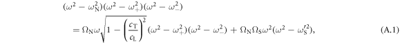
In this appendix we present analytic expressions for the width of the band gaps. The analytical theory represented by equation (1) predicts three resonances:  ,
,  and
and  . For each of these resonances there is a gap,
  ,
,  and
and  , respectively. The upper bound of each gap is the frequency at which the modified Rayleigh mode intersects with the bulk-shear acoustic wave branch,
  . The lower bound of each gap is the frequency of the corresponding resonance. We determine the size of the band gaps analytically by calculating the difference between these two frequencies. Substituting
  into equation (1) gives:
where we define the characteristic frequencies


In order to find  , we can rewrite equation (A.1) as

where  . If we assume
  , the gap can be estimated by

This equation gives 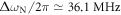 , which agrees well with the exact value of 37.6 MHz, obtained by solving equation (A.1) directly. From the evaluation of equation (A.5), we note that the second term in the brackets is small compared with the first term, so we can simplify the equation further to

This equation gives a value of 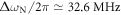 , still in reasonable agreement with the exact value.
A similar calculation can be done for  and
and  . To evaluate
  , we write
Assuming  ,
,  can be expressed as
Similarly,  can be expressed as
