


Abstract
We study theoretically and experimentally the influence of temporally shaping the light pulses in an atom interferometer, with a focus on the phase response of the interferometer. We show that smooth light pulse shapes allow rejecting high frequency phase fluctuations (above the Rabi frequency) and thus relax the requirements on the phase noise or frequency noise of the interrogation lasers driving the interferometer. The light pulse shape is also shown to modify the scale factor of the interferometer, which has to be taken into account in the evaluation of its accuracy budget. We discuss the trade-offs to operate when choosing a particular pulse shape, by taking into account phase noise rejection, velocity selectivity, and applicability to large momentum transfer atom interferometry.
Export citation and abstract BibTeX RIS

Original content from this work may be used under the terms of the Creative Commons Attribution 3.0 licence. Any further distribution of this work must maintain attribution to the author(s) and the title of the work, journal citation and DOI.
1. Introduction
Precision measurements rely on a careful analysis of the relevant noise sources and systematic effects. In the field of inertial sensors, instruments based on light-pulse atom interferometry allow measurements of gravito-inertial effects such as linear accelerations [1–3], rotations [4–6], Earth gravity field [7, 8] and of its gradient [9] or curvature [10]. They have also been used for precise determinations of fundamental constants [11, 12] and tests of the weak equivalence principle (see, e.g. [13–21]), and have been proposed for gravitational wave detection in the sub-10 Hz frequency band [22, 23]. These sensors most often use two counter-propagating laser beams to realize the beam splitters and mirrors for the atomic waves associated to two different momentum states. The stability and accuracy of the sensors critically depends on the control of the intensity and of the relative phase of these two lasers, both spatially and temporally. For example, the spatial profile of the relative laser phase is the main source of systematic effects in most accurate atomic gravimeters [7, 8], and is an important concern in the design of future gravitational wave detectors based on atom interferometers (AIs) [24].
The temporal shape of the light-pulses (i.e. of the laser intensity) driving an AI determines the efficiency of the beam splitters and mirrors acting on the two momentum states of the AI. More precisely, for velocity selective transitions, the transfer efficiency of the pulse is given by the convolution between the velocity distribution of the atoms and the Fourier transform of the pulse shape [25]. Efficient transitions (i.e. high contrasts) can thus be achieved by temporally shaping the pulse intensity and phase, as shown in [26, 27]. Moreover, when driving an interferometer with large momentum transfer (LMT) atom optics, it has been shown that pulses of Gaussian temporal shape significantly improve the transfer efficiency with respect to rectangular pulse shapes [28, 29]. Adiabatic rapid passage (see, e.g. [30]) was also considered in LMT interferometry, but was shown to require stringent control of the laser phase noise compared to pulse shaping [31].
In addition to the influence on the contrast of the interferometer, the temporal shape of the pulse is expected to affect the (frequency-dependent) response of the interferometer to phase fluctuations, which is an important source of instability in AIs. Furthermore, as the phase response of the AI is modified, pulse shaping should introduce a correction to the scale factor of the interferometer, which has to be accounted for in the accuracy budget of atomic sensors.
In this article, we study the phase response of an AI driven by arbitrary temporal light pulse shapes. Our main interest is to highlight the strong difference in the phase response of an AI driven by rectangular and smooth pulse shapes. We concentrate on a few pulse shapes that are representative for the optimization of the following criteria: rejection of high-frequency laser phase (or frequency) noise, velocity selectivity of the pulse, and applicability to LMT interferometry. Experimentally, we focus on the comparison of the phase sensitivity function (section 2) and of the rejection of laser phase noise (section 3) between the two mostly employed rectangular and Gaussian pulses, in order to validate our calculations. In addition to the rectangular and Gaussian pulses, we discuss two other representative pulse shapes: (i) the GSinc pulse, which is the product of a Gaussian and a cardinal sine, and (ii) the Gaussian-Flat pulse (labeled GFlat thereafter) which is a flat pulse with Gaussian edges. For completeness of the presentation, we study in section 4 the influence of pulse shaping on the frequency selectivity, in line with previous works [26, 27]. Finally, we present in section 5 a correction to the interferometer scale factor associated with pulse shaping, and discuss its relevance for different precision measurements involving AI based sensors. We conclude our paper with a discussion of the trade-offs to operate when selecting a given pulse shape for a particular application (section 6).
2. Sensitivity function with arbitrary pulse shape
2.1. Theory
The sensitivity function was first introduced to study the degradation of an atomic clock due to the phase noise of the local oscillator [32], but the idea is more general. It describes the response of an atom interferometer phase to infinitesimal changes of external parameters. We investigate here the response of the AI phase  to an instantaneous variation
  of the relative phase between the two lasers driving the AI, occurring at a given time t. As in previous works [33], we define the sensitivity function as

It can be calculated for an interferometer composed of perfect beam splitters and mirrors using

where  is the Rabi frequency seen by the atoms during the interferometric sequence [34], with
  for
for  . The overall shape of
  depends on the AI configuration, i.e. on the number of light-pulses. In this work, our main interest lies in the effect of temporal pulse shape. Therefore, we consider without loss of generality, a two-light pulse interferometer, i.e. a Ramsey configuration. For a Ramsey sequence with two rectangular
  pulses characterized by a Rabi frequency
  and duration τ separated by Ramsey time T, the sensitivity function reads
where the origin of the time axis is (arbitrarily) aligned with the center of the first light pulse.
We show  as a dashed line in figure 1(a). In the limit of infinitely short laser pulses,
  is box-like, as the interferometer copies the phase jitter of the interrogation laser (
 ) between the two laser pulses.

Figure 1. Sensitivity function  of a Ramsey sequence. (a) Complete
  for two rectangular
  pulses separated by Ramsey time T. (b) Zoom on the rising slope for rectangular (blue) and Gaussian (red) pulses. We compare calculations (lines) according to equation (3) and our measurements (points). Errorbars on the measurements are smaller than the plot symbol.
Download figure:
Standard image High-resolution imageWe show in figure 1(b) a zoom of of the rising slope (i.e. during the first  pulse) of
  for a sequence based on rectangular pulses (blue dashed line) and Gaussian pulses (red dashed–dotted line). We have chosen to use the same peak intensity in our calculation (and our experiments later), and adjust the pulse duration to obtain the desired Rabi angle. This is motivated by the fact that the peak laser intensity depends on the total power available, which is often the limiting experimental factor. The main difference in the sensitivity function takes place around
  , where τ denotes the duration of the rectangular
  pulse. The sudden intensity variation of a rectangular pulse gives rise to a fast rise in the sensitivity function, and a discontinuity in its derivative. This fast rise is in contrast with the gradual change induced by a smooth intensity variation of a Gaussian pulse. Such a difference results in different spectral behaviors of
  for the two pulse shapes, as we will discuss in section 3.
2.2. Measurement of the sensitivity function for rectangular and Gaussian pulses
We measure  using the experimental setup described in [6, 35]. Briefly speaking, we use an atomic fountain to prepare cold cesium-133 atoms. At each experimental cycle, about 106 atoms are prepared into the magnetically insensitive
  ground state and launched into the interferometric zone. The Ramsey pulses are realized via stimulated Raman transitions, using a doubly seeded tapered amplifier [36]. The seeding external cavity diode lasers have a fixed phase relation by means of an optical phase locked loop (PLL) close to the Cs clock transition frequency. Both lasers are about 500 MHz red-detuned from the excited state of the
  line to reduce spontaneous emissions during the Raman transition. At the end of the interferometer sequence, the population in each of the hyperfine ground states N3 and N4 is detected by fluorescence, and the transition probability is obtained by
  .
.
The laser phase jump is implemented by applying a DC voltage  to the feedback port in the PLL through a voltage controlled switch, which is triggered at different times. See figure 2 for the control schematics. The voltage offset corresponds to a phase jump of about 340 mrad. The switch has a delay of
  , whereas the PLL has a locking bandwidth of 1.6 MHz. Thus, the total delay in the phase jump implementation is under
  , much shorter than the duration of the rectangular
  pulse
pulse  (peak Rabi frequency
  ).
).
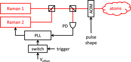
Figure 2. Schematic of the phase jump control. The beat note of two lasers (Raman 1 and 2) is detected on a fast photodiode (PD) and phase locked onto a reference signal at the Cs ground-state hyperfine splitting frequency of about 9.192 GHz. Phase jumps are implemented by sending a DC voltage  to the feedback port of the PLL through a voltage controlled switch. By appropriately attenuating the radio-frequency signal driving the AOM, arbitrary temporal profiles of laser pulses can be sent onto the atoms.
Download figure:
Standard image High-resolution imageWe shape the Raman light pulses by attenuating the radio-frequency signal driving the acousto-optic modulator (AOM), which controls the intensity of the Raman pulses shone on the atoms. A commercial direct digital synthesizer (Rigol 4620) is used to generate a waveform that takes into account the desired waveform (e.g. a Gaussian pulse) as well as the response of the chain of a voltage-controlled attenuator followed by an RF amplifier. This response is calibrated against a monitor photodiode in order to ensure that the intensity of the Raman pulses follows the desired waveform.
With a Ramsey time of T = 20 ms, the phase noise of the clock sequence is about 30 mrad Hz  , which enables a mid-fringe operation of the interferometer. We further stabilize the phase offset of the interferometer by applying a mid-fringe lock [37], which converts the measurement of the atomic transition probability directly to the interferometric phase. This technique is immune to variations in the probability offset and reduces the sensitivity to the noise in the fringe amplitude, thereby allowing a robust measurement of the interferometric phase.
To compare the experimental data with the calculations, we offset the measured phase shift to 0 and normalize by 340 mrad to obtain the experimental  . We display our measurements in figure 1(a) for the complete
  with rectangular pulses [33]. Figure 1(b) shows the rising slope for rectangular (circles) and Gaussian (rectangulars) pulses. The relative phase uncertainty of each measurement is below 4 mrad, i.e. smaller than the plot symbol. The time axis for the experimental data is shifted by
  to account for the delay through the switch and the PLL. Our measurements confirm the temporal form of
  given by equation (3), and well resolve the differences between the two pulse shapes implemented.
3. Frequency response of the AI to pulse shaping
3.1. Calculations
The impact of the sensitivity function on the interferometer phase noise can be more easily understood in Fourier space. According to [33, 35], the variance of the interferometric phase noise can be expressed as

where the transfer function  ,
,  is the Fourier transform of the sensitivity function
  , and
, and  is the power spectral density of the Raman laser phase noise.
We plot in figure 3 the transfer function  as a function of frequency f for a 3 light pulse sequence (
 ) for various pulse shapes: rectangular (blue dashed line), Gaussian (red dashed–dotted line), GSinc (purple dotted line), and GFlat (green). The peak Rabi frequency is the same for all pulse shapes. The calculation is analytic for rectangular pulse and numerical for the other pulse shapes. The Gaussian pulse is truncated at 6 standard deviations on both sides. The definition of the GSinc and GFlat pulse shapes is given in appendix A.
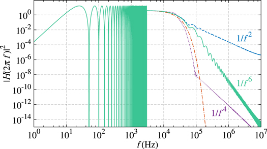
Figure 3. Transfer function  for a 3 pulse AI with T = 20 ms driven by different pulse shapes: rectangular (blue dashed line), Gaussian (red dashed–dotted line), GSinc (purple dotted line), and GFlat (green solid line). The peak Rabi frequency is the same for all pulse shapes.
Download figure:
Standard image High-resolution imageIndependent of the pulse shapes used, the transfer function  is oscillatory with arches spanning
  , i.e. 50 Hz for our choice of T = 20 ms. This is illustrated at low frequency up to 3 kHz, beyond which we plot the mean value over 3 kHz in order to illustrate the general frequency dependence of the envelope.
The difference between the four pulse shapes lies mainly in the low-pass cut-off occurring near the peak Rabi frequency (here 12 kHz). For a rectangular pulse, the high-frequency noise is filtered out with a  scaling of H2, whereas the use of smoother pulses warrants a significantly faster decay, and therefore a better suppression of high-frequency noise. In particular, Gaussian pulses give rise to the strongest high-frequency cut-off in H2. The GSinc pulse gives a similar behavior as the Gaussian pulse around the peak Rabi frequency, before following a
  scaling at high frequency. The frequency at which the slope changes is determined by the width of the Gaussian relative to the length of the sine cardinal (the smaller the width of the Gaussian, the further the change of slope). The GFlat pulse gives rise to
  scaling in H2 beyond the peak Rabi frequency.
To understand the asymptotic behavior of the transfer function qualitatively, we performed calculations with various pulse shapes, including temporally asymmetric pulses, and using different shapes for the  and π pulses. We found that the high frequency behavior is first determined by the steepness of
  at the beginning of the first
  and the end of the last
  pulses. Even faster decay of the transfer function is then related to the steepness of
  at the end of the first
  pulse, the beginning of the last
  pulse, and the π pulse. Further details on this qualitative interpretation in line with equation (2) can be found in appendix B.
3.2. Measurements of the transfer function
We measure the transfer function  for different pulse shapes by realizing a Ramsey sequence (
 ) using co-propagating Raman transitions, with a Ramsey time of
  , and a Rabi frequency of 8.3 kHz. To measure the transfer function, we follow the approach of [33]: we apply a sinusoidal phase modulation of angular frequency ω starting at the first Raman pulse and lasting during the whole interferometer, and measure its effect on the phase of the atom interferometer. We perform two measurements corresponding to two quadratures of the phase modulation, which are added quadratically in order to extract the value of
  . The maximum of
  corresponds to a phase shift of 1.05 rad. The relative uncertainty of the phase measurements are at the level of
  . To show the asymptotic behavior of
  , we measure the position of the maxima of the transfer function over several decades. The measurements are shown in figure 4(a) , together with the calculation presented in the previous subsection, without free parameters. The experimental data and the calculation agree well within the uncertainties of the experimental parameters (
 on the Rabi frequency and
  on the position of the maxima at frequencies above 10 kHz). In particular, the measurements resolve the difference in asymptotic behavior of the three pulse shapes. We also observe that the positions of the zeros of the transfer function are indistinguishable for all pulse shapes at frequencies lower than the Rabi frequency, as illustrated around 8.3 kHz in panel (b).
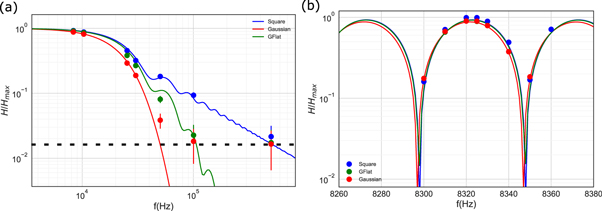
Figure 4. Transfer functions for a Ramsey sequence  with a Rabi frequency of 8.3 kHz, and a Ramsay time of 20 ms. Three pulse shapes are considered: rectangular (total duration of 30 μs), Gaussian, and GFlat. (a) Asymptotic behavior of
  , where the experimental and theoretic data are the maxima of the arches. (b) A zoom around the Rabi frequency. The errorbars correspond to statistical errors at the
  confidence interval. The dashed horizontal line in (a) corresponds to the noise floor of our measurements.
Download figure:
Standard image High-resolution image3.3. Experimental demonstration of noise rejection
To demonstrate experimentally the robustness of smooth pulses against high-frequency laser phase noise (compared to rectangular pulses), we realize Ramsey sequences ( ) with additional relative phase noise in the Raman lasers. The difference between the Ramsey sequence and the 3-pulse sequence (
 ) only lies in the low frequency behavior of the transfer function (at
  ), while the high frequency behavior (for f on the order of and higher than the Rabi frequency) is the same for both sequences. We concentrate on the comparison between Gaussian and rectangular pulse shapes. Adding phase noise is achieved by sending a noisy signal (instead of a switchable DC voltage as illustrated in figure 2) into the feedback port of the PLL. We generate a white noise using a commercial synthesizer, filtered into the 40–300 kHz band pass and amplified using a commercial low-noise amplifier. By varying the amplifer gain, we control the additional phase noise of the Raman lasers, giving rise to the power spectral density shown in figure 5(a). For each noise level, we measure the short-term phase stability of a Ramsey sequence (T = 20 ms) with rectangular (circles) and Gaussian (rectangulars) pulses, as shown in figure 5(b). In comparison, Gaussian pulses consistently rejects a significant fraction of the additional noise.

Figure 5. (a) Power spectral density of the laser phase noise recorded with a spectral analyzer with a resolution bandwidth of 1 kHz. The yellow line shows the spectrum without additional noise (gain = 0 in the low-noise amplifier), whereas the purple, green and cyan lines correspond to increasing noise levels (amplifier gain = 2, 5, and 10). (b) Short-term phase stability of a Ramsey interferometer. We overlay our measurements (points) with calculations (lines) for rectangular (blue) and Gaussian (red) pulses. The errorbars correspond to statistical errors at the  confidence interval.
Download figure:
Standard image High-resolution imageWe calculate numerically the induced phase noise according to equation (4), by numerically integrating over the 10 kHz–2.5 MHz range. The contribution of frequencies out of this band is negligible. The total noise is  , where
  is our measured detection noise. To account for the uncertainty in the absolute phase noise level applied to the interferometer, we multiply the phase noise PSD of figure 5(a) by a global factor. This factor is obtain by matching the calculation and measurement for upper right point in figure 5(a), which is almost exclusively influenced by phase noise (and not detection noise). Apart from this global factor common to both pulse shapes, there are no free parameters. The calculation follows well the experimental data, and shows how the Gaussian pulse rejects the high frequency phase noise, above the Rabi frequency.
3.4. Discussion and applications to inertial sensors and optical clocks
The strong rejection of the relative laser phase noise by a smooth pulse (Gaussian, GSinc, GFlat) at frequencies higher than the Rabi frequency will help designing optical PLLs for AI experiments, as it relaxes the requirements on the PLL bandwidth. Regarding the limitation to the sensitivity of cold atom gravimeters due to Raman laser phase noise, we calculate the noise rejection in state of the art instruments. For the work presented in [38], we compute a phase noise of 7.5 mrad per shot (assuming a π rectangular pulse with a duration of 15 μs), in agreement with the measured short term stability. Using a GFlat pulse yields a noise of 6.1 mrad, and a Gaussian pulse reduces this contribution to 5.9 mrad per shot. For the work presented in [39], the rectangular pulse corresponds to a phase noise of 1.1 mrad per shot, which will be reduced to 0.5 mrad per shot when using GFlat or Gaussian pulses.
In AIs driven by Bragg diffraction, the relative phase noise between the two Bragg lasers is not a concern, since the two momentum states used in the two interferometer arms correspond to the same internal energy state. However, because of propagation delay from the atoms to the mirror which retro-reflects the Bragg lasers, the laser frequency noise converts into phase noise on the AI [40]. Such noise is a major concern in long baseline AI gradiometers, e.g. in gravitational wave detectors based on AIs [23, 41]. Smooth pulses can therefore relax the requirements on the laser frequency noise at high frequencies (above the Rabi frequency, i.e. above typically 10–100 kHz).
We also investigate the potential interest of temporally shaping pulses to improve the stability of optical clocks. The stability of optical clocks critically depends on the frequency stability of the interrogation laser [42], the design of which requires careful attention [43]. In that context, we found that pulse shaping in clocks is less interesting than in AIs. The reason is that the relevant transfer function for the measurement of frequency (instead of phase) is  , which scales as
  (for a rectangular pulse) after the cut-off given by the pulse Rabi frequency
  . For white frequency noise, the contribution of high frequencies (
 ) is thus 1/3 of that of low frequencies (
 ), in power of the noise. Therefore, faster decay (than
  ) of the transfer function does not significantly impact the stability. Pulse shaping can however be used to relax the constraints on potential spurious high frequency noise components in the clock laser, e.g. in field applications or compact clock design [44].
4. Frequency selectivity of the pulse
We investigate in this section the frequency selectivity of the pulse shapes studied in this article, in line with previous works [26, 27]. We measure the influence of the pulse shape on the frequency selectivity of the pulse, by varying the Raman laser frequency difference and measuring the transition probability. The results are presented in figures 6(a) and (b) for a  pulse and a π pulse correspondingly, for the four pulse shapes investigated in the previous section: rectangular, Gaussian, GFlat, and GSinc.
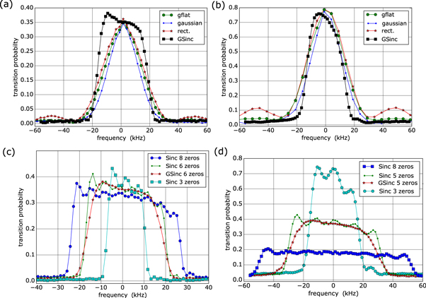
Figure 6. Spectroscopy of different pulse shapes. (a)  pulse. (b) π pulse. In both cases, the duration of the rectangular pulse is 30 μs. The peak power is the same for all pulse shapes in (a), and the same for all pulse shapes in (b). In (c), the total duration of each pulse is
  and the peak power is varied to perform a
  pulse. In (d), the peak power is kept constant and the pulse duration is kept constant to 150 μs. The maximum measured probabilities for the
  and π pulse are different from the ideal values of, respectively, 0.5 and 1 because of experimental imperfections (inhomogeneous Rabi frequency and imperfect normalization of the transition probability).
Download figure:
Standard image High-resolution imageThe GSinc pulse is technically more difficult to implement than the other pulse shapes as it requires the introduction of phase jumps of π at the points in time corresponding to the zeros of the power envelope in order to reverse the sign of the effective Rabi frequency (see figure A2 in the appendix for the time trace of the Sinc pulse). The π phase jumps are applied on the relative phase between the two Raman lasers through the phase lock loop, in a similar way as for the measurement of the sensitivity function presented in section 2.2. For the data presented in panels (a) and (b), the GSinc is the product of a Gaussian and of a Sinc function with 5 zeros on each side of the maximum (see appendix A). The total duration of the pulse is 300 μs, and the peak power is the same as for all pulse shapes. The standard deviation of the Gaussian multiplying the Sinc function is 1/6 of the total duration (i.e. 50 μs).
The experimental data are in agreement with the theoretical expectation, shown in figure 7, that the spectroscopy is the Fourier transform of the pulse shape. In particular, the side lobes associated to the rectangular pulse are absent in the GFlat, Gaussian, and GSinc pulses. The measurements also resolve the larger width of the GFlat pulse compared to the Gaussian pulse. Finally, the GSinc pulse clearly shows sharper edges than the other pulse shapes. The asymmetry in the GSinc spectroscopy is not fully understood: we think that it is due to a nonlinearity in the acousto-optic modulator which is driven for a longer duration for the GSinc pulse (300 μs) compared to the other pulse shapes (the spectroscopy were less asymetric when using shorter pulses).

Figure 7. Calculations of the line shapes. The panels correspond to the measurement shown in figure 6. The parameters are fixed to the values measured in the experiment (pulse duration, peak Rabi frequency). Note that the maximal probability of transition in this ideal calculation is 0.5 for the  pulses and 1 for the π pulses.
Download figure:
Standard image High-resolution imageWe investigate experimentally in further details the influence of the number of zeros in the Sinc pulse on the sharpness of the spectroscopy. The results are shown in figures 6(c) and (d). Panel (c) shows the measurements for a  pulse where the total duration of all pulses is kept constant to 300 μs, and the peak power is varied. Panel (d) shows measurements were the peak power is kept constant and the pulse duration is kept constant to 150 μs.
In conclusion, the Sinc and GSinc pulses exhibit an almost flat response to detuning, and a sharper decay than the other pulse shapes. They therefore optimizes the velocity acceptance of the pulse, at the expense of more complexity in the implementation.
5. Scale factor of the interferometer
The finite duration of the light pulses influences the scale factor of atom interferometers, i.e. their response to inertial effects. The interferometer phase Φ is related to the relative laser phase  through the sensitivity function as
  . Without loss of generality, we look at the example of a Mach–Zehnder-like interferometer sequence, where there are three light pulses (
 –π–
–π– pulses) separated by T between each consecutive pulse pairs. See figure 8 for an illustration. The finite duration τ of the
  (rectangular) pulses modifies the scale factor of an atom accelerometer from
  to
to  , with
  [45]2
. For experiments where the inertial effect is inferred from a phase measurement, such a change of scale factor has to be taken into account when evaluating the accuracy budget.
[45]2
. For experiments where the inertial effect is inferred from a phase measurement, such a change of scale factor has to be taken into account when evaluating the accuracy budget.
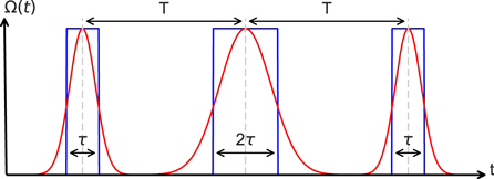
Figure 8. Illustration of the three-pulse interferometer sequence for rectangular and Gaussian pulse shapes. The pulse separation T denotes the time elapsed between the center of two consecutive light pulses, and τ is the duration of the  rectangular pulse.
Download figure:
Standard image High-resolution imageFurthermore, by modifying the temporal pulse shape, the scale factor  differs from that of rectangular pulses
  . Since
  is typically on the order of
  or smaller, the relative correction
  scales linearly with
  , and can be evaluated numerically with the appropriate form of
  . For example, for T = 100 ms and a peak Rabi frequency of 12.5 kHz (
 rectangular pulse), this correction amounts to
  for a sequence of Gaussian pulses,
  for GSinc pulses and
  for GFlat pulses.
6. Discussion
We summarize the properties of the four pulse shapes studied in this article in table 1. We report (i) the velocity selectivity of a  pulse (defined as the bandwidth in units of the peak Rabi frequency, see appendix A), (ii) the suitability for LMT interferometry, (iii) the rejection of phase noise at high frequencies (according to section 3), and (iv) the ease of implementation. The main focus of this article was on the phase noise rejection. Details on the velocity selectivity are given in appendix A.
Table 1. Summary of the properties of the pulse shapes studied in this article. The bandwidth is defined as the two-photon detuning (in units of the peak Rabi frequency) where the transition probability falls to 50% and 95% of its maximum value. The phase noise rejection (weak/strong) is defined according to the decay of the transfer function above the Rabi frequency, as shown in figure 3.
| Pulse | Bandwidth (50%  95%) 95%) |
LMT | Noise rejection | Ease of implementation |
|---|---|---|---|---|
| Rectangular | 1.73  0.49 0.49 |
Not suitable | Weak, 
|
Easiest |
| Gaussian | 1.31  0.36 0.36 |
Suitable | Strong | Medium |
| GSinc | 1.73  1.01 1.01 |
Suitable | Strong | Difficult |
| GFlat | 1.65  0.47 0.47 |
Suitable |

|
Medium |
Regarding LMT applications [28, 29], we extended the numerical calculations performed in [46] to implement arbitrary pulse shapes, and computed the Rabi oscillations for  LMT atom optics. We found that all smooth pulse shapes (Gaussian, GSinc, GFlat) support LMT beam splitters for pulse durations of few inverse peak Rabi frequency, in contrast to the rectangular pulse.
Regarding the ease of implementation, the rectangular pulse is the most simple as it only requires a digital signal to drive, typically, a voltage controlled oscillator. The implementation of the Gaussian or the GFlat pulse shapes require a waveform generator and can be realized with relative ease. The GSinc pulse (characterized by negative values in the Rabi frequency) can be implemented experimentally by setting π phase shifts at the points of zero crossing. It requires a waveform generator in combination with a sufficiently fast phase modulation, and is thus more challenging to implement.
Disregarding the implementation of the pulse shapes, the GSinc pulse is suited for all applications, as it presents the largest velocity acceptance, can efficiently perform LMT transitions, and rejects high frequency laser phase noise. In comparison, although the GFlat pulse has a reduced velocity acceptance, it fulfills all other criteria, and can therefore be considered as a good compromise for various applications.
As a final note in this discussion, we remark that the interest of using an optical cavity to drive the light pulses in an AI has been raised recently [46, 47]. The power enhancement at the cavity resonance requires sufficient finesse  , which modifies the intensity build up time
  , and therefore the temporal shape of the pulse. The effect on the pulse shape will be particularly important in long-baseline gradiometers using AIs in an optical cavity, as planned in [41], where
  may be of the order of the pulse duration (i.e. few μs). We computed the sensitivity function for such a cavity-like pulse shape (see appendix C), which shows a
  high-frequency behavior.
7. Conclusion
We investigated the influence of temporally shaping the light pulses on the response of an AI. The main focus of our study was on the modification of the AI sensitivity function to phase, at frequencies of the order of and higher than the effective Rabi frequency. We demonstrated that smooth pulse shapes allow for a significant rejection of high frequency phase fluctuations compared to rectangular pulses. We also presented the modification of the scale factor of the AI due to pulse shaping, which has to be considered in the evaluation of systematic effects of AI sensors. We finally discussed the trade-offs between the different representative pulse shapes considered in the article. One important conclusion of our study is that the rejection of high frequency phase fluctuations can be achieved with a minor effect on the velocity acceptance of the pulse by employing, for example, a GFlat pulse shape, which can also efficiently perform LMT beam splitters.
In the context of LMT interferometry, future work should study the modifications of the sensitivity function for AIs driven by LMT beam splitters (see [48] for a preliminary analysis) and the influence on the rejection of the laser frequency noise, as has been done, for example, for laser intensity noise induced light shift [49].
Acknowledgments
We acknowledge the financial support from Ville de Paris (project HSENS-MWGRAV), FIRST-TF (ANR-10-LABX-48-01), Centre National d'Etudes Saptiales (CNES), DIM Nano-K, and Action Spécifique du CNRSGravitation, Références, Astronomie et Métrologie (GRAM) and Sorbonne Universités (project LORINVACC). BF is funded by Conseil Scientifique de l'Observatoire de Paris, NM by Ville de Paris, DS by Direction Générale de l'Armement, and MA by the EDPIF doctoral school. We thank Azer Trimèche for his work on the programming of the arbitrary waveform generator used in this work, Pierre Dussarrat for pointing the GSinc pulse to our attention, and Leonid Sidorenkov for his contributions in the completion of this work.
Appendix A.: Definition of the pulse shapes
We define the time-dependent Rabi frequency as

with  the peak Rabi frequency. The pulses are defined by the function
  with maximal amplitude 1.
The GSinc pulse is defined as

With  , t1 the time of the first zero of the sinc,
  the standard deviation of the Gaussian modulation. The total pulse duration is defined as
  . In figure 3 the parameters of the GSinc pulse are n = 6 and
  .
.
The GFlat pulse is even and defined as

where t0 is the half length of the plateau, and  is the standard deviation of the Gaussian. The total pulse duration is defined as
  . In the main text, we consider GFlat pulses with r = 1 and n = 6.
The pulse shapes are illustrated in figure A1.

Figure A1. Illustration of the different pulse shapes considered in this article: rectangular (plain blue line), Gaussian (green dashed), GFlat (violet dotted–dashed), GSinc (dotted red). Note that the peak Rabi frequency is kept constant for all pulse shapes. For ease of illustration, we have cropped the GSinc pulse to its center part in the main panel. The inset shows the full GSinc pulse shape. The time axis is in units of the inverse Rabi frequency.
Download figure:
Standard image High-resolution imageIn section 4 we study experimentally several Sinc pulse shapes with different number of zeros on each side of the maximum. As an illustration of implementation of such pulses, a time trace of a Sinc pulse with 8 zeros on each side of the maximum is shown in figure A2.

Figure A2. Time trace of the sinc pulse with 8 zeros on each side of the maximum. The blue line shows the voltage recorded by the photodiode which monitors the power of the Raman beam. The green trace shows the digital signal which triggers phase jumps of π applied to the phase lock loop. The inset is a zoom on the zeros of the power and on the phase jumps.
Download figure:
Standard image High-resolution imageAppendix B.: Details on the qualitative study of the influence of the pulse shape on the transfer function
The high frequency behavior of the transfer function can be qualitatively understood from the pulse shape according to the position of the pulses in the interferometric sequence. We recall that the transfer function is  , where
  is the Fourier transform of
  , which is itself the sine of the integral of the time-dependent Rabi frequency, see equation (2). We define
  .
.
Our first observation, illustrated in figure B1(left), is that a decay faster than  can be obtained by smoothing the beginning of the first
  and the end of the last
  pulses. At these points in time, where
  , the sensitivity function can be Taylor-expanded as
  . A rectangular pulse results in a triangular form of
  , giving rise to a
  dependence in
  and hence to a
  dependence in
  . In contrast, smooth pulses are characterized by a slower growth of
  and hence a faster decay of
  . This is illustrated in figure B1(left) by calculating the transfer function using half Gaussian pulses for the
  pulses and a rectangular π pulse.
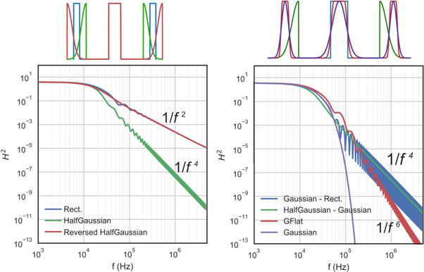
Figure B1. Illustration of the behavior of  at high frequency using different sequences of pulses. The calculations are for a 3 pulse interferometer with 12 kHz peak Rabi frequency and T = 20 ms, using different pulse shapes. The top panel shows the considered pulse sequences. Left: evolution from the
  scaling to the
  scaling, which occurs when smoothing the outer parts of the interferometer pulses, i.e. the beginning of the first
  pulse and the end of the last
  pulse. Right: evolution from the
  scaling to even faster decays when smoothing the inner parts of the interferometer pulses.
Download figure:
Standard image High-resolution imageEvolution from  to a faster decay is governed by the end of the first
  pulse, the beginning of the last
  pulse, and the beginning and end of the central π pulse. At these positions,
  , and the sensitivity function can be approximated by
  . Here the leading order of the time-dependence is quadratic, which explains why the influence of this part of the pulses has a weaker influence on the high frequency behavior. The rectangular π-pulse, for example, results in a parabolic shape of
  , yielding a
  dependence of
  . Figure B1(right) illustrates the need to smooth these parts of the pulses in order to obtain a decay faster than
  in the transfer function.
Appendix C.: Transfer function for an atom interferometer in an optical cavity
We present in figure C1 the temporal shape (top), the velocity selectivity (middle) and the transfer function for a pulse shape resembling the response of an optical cavity. We assumed an intensity build up time of  . Compared with rectangular pulses (blue), cavity pulses is more selective to detuning but rejects better the high-frequency laser phase noise.

Figure C1. (Top) Shape of a cavity-like pulse and (middle) selectivity to detuning for a  pulse. Here
  . We show the shape of a rectangular pulse for comparison. Bottom:
  in a 3 pulse interferometer with 12 kHz peak Rabi frequency and T = 20 ms. We show here again the response of the rectangular and Gaussian pulses for the ease of comparison.
Download figure:
Standard image High-resolution image
Footnotes
- 2
The correction in the main text corresponds to equation (2.45) on page 38 with T defined as the time elapsed between the center of adjacent pulses.