


Abstract
Epidemic spreading processes on multiplex networks have richer dynamical properties than those on single layered networks. To describe the intertwined processes on such networks, heterogeneous mean field (HMF) approach for continuous-time processes and microscopic Markov chain approach for discrete-time processes have been proposed. However, it has been shown that the time evolution of infected individuals and the final epidemic size obtained from these approaches have noticeable discrepancy comparing to those from Monte Carlo simulations. In this paper, we extend the approach of effective degree theory (EDT) on multiplex networks. We will show that predictions obtained from the EDT have excellent agreement with Monte Carlo simulations. Moreover, since the dynamics on multiplex networks involve more dynamical variables, which may invoke more computations, to reduce the computational burden, we further develop an approach based on partial effective degree theory (PEDT) for analyzing the dynamics on multiplex networks, where one layer adopts EDT and the other layer adopts the HMF. Our results show that PEDT has a good performance in predicting the target dynamical process.
Export citation and abstract BibTeX RIS

Original content from this work may be used under the terms of the Creative Commons Attribution 3.0 licence. Any further distribution of this work must maintain attribution to the author(s) and the title of the work, journal citation and DOI.
1. Introduction
Epidemic spreading is an extensively studied topic in the field of complex networks [1, 2]. On the practical side, the study of this topic contributes to the understanding of behaviors of epidemics, while on the theoretical side, it provides a simple dynamical framework to demonstrate rich phase diagrams for analysis. Several mathematical models have been proposed to describe common infectious diseases, including two-state SIS model and three-state SIR model with S standing for susceptible, I for infected, and R for recovery in the epidemiological terminology [3, 4]. A variety of methods have been developed to analyze the epidemic spreading processes, including generating function [5, 6], pair-approximation [7], heterogeneous mean field theory [8–10], probability generating function [11, 12], and branching process approximation [13, 14].
Beyond the studies on single layered networks, growing attention has been focused on epidemic spreading on multiplex networks [15–17]. Recently, the intertwined effect of epidemic spreading and information diffusion on multiplex networks [18], where the microscopic Markov chain approach (MMCA) is taken to understand the interplay between an epidemic spreading process and an awareness spreading process. Further, other effects are studied under this framework, such as the effect of mass media [19], awareness cascade [20], and heterogeneous responses [21]. The relevant analysis are mostly based on MMCA.
The MMCA has been previously proposed on single layered quenched networks for discrete-time epidemic processes [22, 23]. However, it has been shown that the predictions of the time evolution of epidemics and the final epidemic sizes have noticeable discrepancy comparing to the Monte Carlo simulations, especially when the infection is slightly above the epidemic threshold [24]. This defect comes from neglecting the correlation of the underlying dynamics. Since accurate prediction of epidemic processes is important and valuable in both theoretical and practical considerations, an effective degree theory (EDT), which considers the dynamical correlations, is proposed for gaining more accurate predictions in [24]. An approach, similar to the EDT, while on a node-based and link-based perspective is also proposed for this purpose [25]. In single layered networks, the EDT has been developed for SIS and SIR epidemics models [26, 27], a wide class of binary-state dynamics [28, 29], and correlated networks [30]. However, despite the rapid advance in the studies about spreading dynamics on multiplex networks, an approach to accurately predict relevant behavior is still in demand, which deserves in-depth investigations.
In this paper, we develop an EDT on multiplex networks based on the UAU-SIS model [18], where the epidemics and the awareness dynamics co-evolve. Our results show that the new approach could predict the dynamics in high accuracy, outperforming both HMF and MMCA. Moreover, to enhance the efficiency of the approach, we further develop a partial effective degree theory (PEDT), in which the dynamics one layer adopts EDT and the dynamics in the other layer adopts HMF. We show that the PEDT provides satisfactory accuracy for the dynamics in the layer adopted EDT meanwhile systematically reducing the dimensions of the governing equations in computations.
The paper is organized as follows. In section 2, we introduce the two-layered networks based on the UAU-SIS model. In section 3, we provide the EDT for the model, and in section 4 we show the numerical results. In section 5, we propose the partial EDT for the model. Finally, we conclude the paper by section 6.
2. Model
To start, recall the UAU-SIS model [18, 19]. Specifically, consider a multiplex network composing of two layers, each layer has the same number N of individuals with different connectivity configurations. In one layer (the upper layer in figure 1), an individual could be in two states: aware (A) and unaware (U), denoting whether it is aware of certain news, i.e. the spreading of an epidemic. The state of an individual could evolve between U and A, thus forming a UAU process. For simplicity, this layer is referred to as awareness layer. In the other layer (the lower layer in figure 1), epidemic spreads and an individual could be either infected (I) or susceptible (S), forming an SIS process. For simplicity, this layer is referred as epidemic layer. Combining the two layers, at any time each individual in this multiplex network can be in one of the four types of states: unaware and susceptible (US), unaware and infected (UI), aware and susceptible (AS), aware and infected (AI).
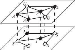
Figure 1. Model of spreading dynamics on a multiplex network. The upper layer represents the network where the awareness of the epidemic diffuses. Nodes in this layer can be in two types of states: unaware (U) and aware (A). The lower layer represents the network where the epidemic spreads. Nodes in this layer can be in two types of states: susceptible (S) and infected (I). Therefore, a node could be in four types of states: unaware and susceptible (US), unaware and infected (UI), aware and susceptible (AS), and aware and infected (AI).
Download figure:
Standard image High-resolution imageDetails of the dynamics on the multiplex network are as follows: for the UAU process, the dynamics are composed of two parts. On one hand, an unaware individual (node) may become aware due to two reasons: first, it may be informed by its aware neighbours, and each aware neighbour could send the news to it at a rate α. Second, if an unaware individual has been infected, it may be aware of the epidemic at a rate τ due to self-awareness, which reflects a direct impact from the epidemic layer. On the other hand, an aware individual may return to be unaware because of forgetting the news at a rate f. For the SIS process, a susceptible individual can be infected by an infectious neighbour. If this susceptible individual is unaware (aware) of the epidemic, i.e. an US (AS), the infection rate by an infected neighbour will be  (
( ), where
  as an effect of preventive measures taken by aware ones. For simplicity, assume
  with a reduction coefficient
 ![$\theta \in [0,1]$](https://content.cld.iop.org/journals/1367-2630/21/3/035002/revision2/njpab0458ieqn5.gif) , where
, where  will be abbreviated as β in the rest of the paper. This reduction coefficient θ reflects the direct impact from the awareness layer. In addition, an infected individual can be recovered to become susceptible at a rate r.
3. Effective degree theory
The EDT is now extended to be on multiplex networks. A feature of EDT is that the states of the individuals, the number of their neighbours and related dynamical states are also taken into account, based on which the dynamical correlation is considered. To realize this feature, individuals are grouped into classes of  , where
  and
and  , and the subscripts u, a, s, i denote the numbers of unaware, aware, susceptible, infected neighbours they have, respectively.
If not causing confusion,  are used also to denote the fraction of individuals in respective classes. Thus, one may immediately obtain the conservation law as
  . Then suppose that initially a fraction a0 of individuals are aware of the epidemics and a fraction i0 of individuals are infected, which are randomly distributed in the respective layers with no correlations. Then,
  , where
  denotes the fraction of individuals in the state X(Y) with a number of u unaware (s susceptible) and a aware (i infected) neighbours. Suppose that the degree distributions of the awareness layer and epidemic layer are pi and qk, which denote the fraction of individuals who have i and k neighbours in the respective layer. Then, one obtains

In this paper, the dynamics are in continuous-time processes and the EDT approach to be developed will be presented by a set of ordinary differential equations (ODEs). To simplify the analysis, the whole process is separated into four sub-processes, named the infection process, recovery process, awareness process, and forgetting process, respectively. In the continuous-time process, the time interval of each update is very small. Thus, the nonlinear impacts among different sub-processes in a short time interval could be ignored, and the update of the whole process is equivalent to the summation of those on the four sub-processes. Therefore, for each class of individuals, one first calculates their variations in the four sub-processes, respectively, and then sums them up to obtain the variation of the whole process. Denoting the differential operators of the ODEs of the four sub-processes and the whole process as  ,
,  ,
,  ,
,  , and d/dt, respectively, one has
  . All possible state transitions for individuals in a certain class of
  is presented in figure 2, and in the following we will derive the governing equations of these sub-processes accordingly.
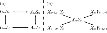
Figure 2. Possible states transitions for individuals in the class of  where
where  and
and  . (a) The possible state transitions on individuals in the class of
  . (b) The possible state transitions on a neighbor of individuals in the class of
  .
.
Download figure:
Standard image High-resolution imageNow, the EDT of the four sub-processes is shown in sequence. Start from the infection process. Since, in the continuous-time description, the possibility of two events happen in one time interval can be ignored, the change in the states of an individual's neighbours due to the infection process could only be the case of  , i.e. an susceptible neighbour changes to be infected through the infection. However, since this susceptible neighbour could be either US or AS, the estimation of its changing rate should account for the different infection rate β or θβ due to the two kinds of states. Here, mean field approximation is used to estimate its changing rate. This susceptible neighbour could be either an
  or a
or a  one. Suppose that it is
  . Note that the possibilities of a
  individual reached by this neighbour through a certain link equals
  . Thus, for a
  individual, the rate that it has an
  neighbour meanwhile this neighbour is infected equals
  . Similarly, when this neighbour is
  the corresponding rate equals
  . Summing all the possible classes of the neighbours gives the effective infection rate of a susceptible neighbour of a
  individual, defined as
  , as follows:

It is not difficult to find that a susceptible neighbour of an  individual has the same effective infection rate
  . With a similar reason, the effective infection rate of a susceptible neighbour of a
  or
or  one is defined as

Thus, one obtains the evolution equations of the infection process as follows:


Here, the second term on the right-hand side of equation (4a) describes the event that one of the susceptible neighbours of a  individual becomes infected at a rate
  and hence
  changes to
  , leading to a subtraction from the value of
  .
.
The recovery process is relatively simple and its evolution equations are given as follows:


Similarly to the infection process, in the awareness process one can define the effective awareness rate of an unaware neighbour reached by an unaware and an aware individual as  and
and  , respectively, as follows:


Moreover, as a UI individual may change to AI at a rate τ due to self-awareness, this effect could also cause a change in the states of an unaware neighbour. Define the effective changing rate of an unaware neighbour reached by an unaware and an aware individual due to this event as  and
and  , respectively, as follows:


Thus, the evolution equations of the awareness processes are


Finally, the evolution equations of the forgetting processes are given as follows


4. Numerical results
The performance of the EDT on a multiplex network is examined in which each layer is generated with (i) Erdös–Rényi model whose degree distribution is  in the limit of
  , and (ii) Configuration model with the truncated power-law degree distribution, where
  when
when  and
and  otherwise. For the convenience of discussion, the two kinds of networks are denoted as ER network and PL network, respectively.
Since the developed method is for continuous-time processes, in order to fulfill this condition small dynamical parameters are used to realize the process, so that in each time step the increments of the variables are small and higher-order terms can be neglected. Thus, in the simulation, the values of the parameters a, f, b, r, and τ are set in an order of 10−3.
Figure 3 shows the results of time evolutions of the fraction of aware individuals  and the fraction of infected individuals ρI(t) for the two kinds of networks. For easy comparison, besides the results of the simulation and the EDT, the results of heterogeneous mean field method (HMF) and MMCA are also presented. The governing equations of HMF and MMCA can be found in appendices A and B, respectively. One can see that the EDT has an excellent agreement with the simulations, while both HMF and MMCA overestimate the dynamics. It is noted that MMCA is developed for the discrete-time process which contains non-perturbative formulations. In the continuous-time limit, the impact of non-perturbative formulation will fade away, reflected by the similar behaviors of the two curves of HMF and MMCA in figure 3.
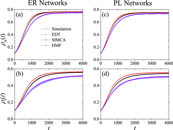
Figure 3. Time evolutions of the fractions of aware nodes  and infected nodes
  for ER networks (a) and (b) and PL networks (c) and (d), respectively. Results are obtained from numerical simulations (blue circles), EDT (magenta curves), MMCA (black curves), and HMF (red curves). The ER network is constructed using the Erdös–Rényi model with average degree 4, and the PL network is constructed using the uncorrelated configuration model with power-law degree distribution
  , where
  and
and  . The network size is N = 10 000. Results are obtained with averaging on 100 different realizations. Other parameter values are
  ,
,  , and
, and  .
.
Download figure:
Standard image High-resolution imageThe final sizes of aware individuals  and infected individuals
  in the steady states of two kinds of networks are shown in figure 4. One can also find an excellent agreement between the Monte Carlo simulations and the EDT. The results of HMF and MMCA also overestimate the dynamics and overlapped to each other.
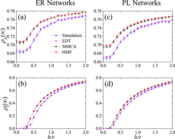
Figure 4. The steady fractions of  and
and  after the transient process as a function of infection rate b, where (a) and (b) for ER networks, (c) and (d) for PL networks. The multiplex networks and other parameters are the same as those in figure 3.
Download figure:
Standard image High-resolution image5. Partial EDT
In the above proposed EDT, there are four variables, u, a, s, and i, corresponding to the numbers of four types of neighbours in concern. Thus, the computational cost will scale as  with kmax being the maximum degree. Therefore, when kmax is large, for example in the extreme case where kmax reaches the upper bound of the degree range for uncorrelated networks in the configuration model [1], i.e.
  , the computational efficiency will not have prominent advantage compared to simulations. In order to increase the computational efficiency, consider a PEDT for multiplex networks. In this method, EDT is adopted for one layer and HMF is for the other layer. Since in the UAU–SIS model, the epidemic dynamics is the target process to be understood and the awareness dynamics is the auxiliary process to better understand the epidemic dynamics, we here adopt EDT for the epidemic layer and HMF for the awareness layer. Specifically, the individuals are grouped into in the classes
  , where k denotes the number of neighbours in the awareness layer and the meaning of other symbols are the same as those in the previous sections. Similarly, one can obtain the initial condition and the evolution equation for PEDT, which are provided in appendix C.
Figure 5 shows the results of the Monte Carlo simulation, EDT, and PEDT for comparison. One can observe that the results of  and
and  for EDT and PEDT have prominent discrepancies. While the results of
  and
and  for EDT and PEDT are well matched. Other parameters have been examined and similar results are obtained. These results show that, although the accuracy in predicting the dynamics of awareness is damaged because of the simple HMF approach, the accuracy in predicting the epidemic dynamics is still preserved. According to the performance of PEDT, this approach may serve as a compromise scheme, where the accuracy is kept in the epidemic layer while the efficiency of the prediction is significantly increased by sacrificing the accuracy of the prediction in the other layer.

Figure 5. The steady fractions of  and
and  after the transient process as a function of self-awareness rate τ for different θ, where (a) a for ER networks, (b) i for ER networks, (c) a for PL networks, and (d) i for scale-free networks. The multiplex networks and other parameters are the same as those in figure 3.
Download figure:
Standard image High-resolution image
6. Conclusion
In summary, in this paper we have developed an effective degree theory (EDT) for studying epidemic spreading dynamics on multiplex networks. We present the new approach on the basis of UAU–SIS model [18]. In this model, a multiplex network is composed of two layers. One is the epidemic layer where an epidemic spreads, while the other is the awareness layer where the awareness of the epidemic diffuses. The dynamics of the epidemic are described by the susceptible-infected-susceptible (SIS) model, and the dynamics of the awareness is described by the unawareness-awareness-unawareness model (UAU). These two layers interact with each other through the reduction of infection rate in the epidemic layer and the self-awareness process in the awareness layer. In presenting the EDT we separate the whole dynamical process into four sub-processes, which are infection process, recovery process, awareness process, and forgetting process. The key step of EDT is to consider the dynamical states of the neighbours of an individual so as to take into account the dynamical correlation of the dynamics. To grasp this property, we classify the individuals according to their dynamical states and the dynamical states of their neighbours in the two layers, respectively, which correspondingly raises four dimensional quantities to account for the sizes of these classes. The developed EDT gives the evolution equations of these quantities.
In the model for a susceptible individual, whether or not it is aware or unaware of the epidemic may result in different infection rates. To account for this effect of different infection rates on a susceptible neighbour, in our approach we use mean-field approximation and propose an effective infection rate to measure the related changing rates. In a similar manner, we further propose an effective awareness rate and an self-awareness rate to describe the relevant changing rates of the neighbours. Our results show that the proposed EDT on multiplex networks successfully predicts the dynamical behavior in a high accuracy. Since the prediction of spreading dynamics on multiplex networks is a more challenging task compared to that on single layered networks, our approach provides a useful tool for future studies on this topic.
We also manifest the performances of the heterogeneous mean field theory (HMF) and MMCA for comparison. We show that these two methods systematically overestimate the epidemics. Since the two methods neglect the dynamical correlation of the dynamics, where an infected individual is more likely to connect with an infected neighbour because it may be infected by the neighbour previously, the number of susceptible neighbours will be overestimated, and consequently it overestimates the whole extent of the epidemics. Besides, as the MMCA is a non-perturbative approach for discrete-time processes, it is expected to return to HMF in the continuous-time limit, which has also been verified in this work.
Since EDT of multiplex networks needs to consider more variables than single layered networks, the computational efficiency of the approach could be an important concern especially when the maximum degree of the individuals is large. Thus, it could be useful to find a method to further improve the efficiency of the theory. For this purpose, we propose a PEDT. In this approach, the epidemic dynamics in the epidemic layer is analyzed by EDT and the awareness dynamics in the awareness layer is analyzed by HMF. The results show that the prediction of the epidemic dynamics remains in high accuracy, meanwhile the computational efficiency of the approach is significantly improved by sacrificing the accuracy in the other layer where the HMF is adopted.
Acknowledgments
This work is supported by the Natural Science Foundation of China (Grant Nos. 61503110), the Natural Science Foundation of Zhejiang Province (LQ16F030006), the Hong Kong Research Grants Council under the GRF Grant CityU (11200317) and the China Scholarship Council Fund (201708330535). The Boston University Center for Polymer Studies is supported by NSF Grant PHY-1505000 and by DTRA Grant HDTRA1-14-1-0017.
Appendix A.: Heterogeneous mean field theory
In this approach, nodes are classified according to their degrees in different layers.  denotes the fraction of nodes in state X (either U or A) and state Y (either S or I) with i neighbors in the awareness layer and k neighbors in the epidemic layer. Thus, the governing equations are given by


where  and
and  , and
, and 
 is the average degree of the awareness (epidemic) layer. The parameters have the same definitions as those in the main text.
Appendix B.: Microcopic markov chain approach
In this approach, the possibility of an individual i lingered on the four states  at time t are denoted as
  ,
,  ,
,  and
and  , respectively. Moreover, the probabilities for individual i not being informed by any of its neighbours, defined as ri(t), not being infected by any of its neighbours if i is aware of the epidemics, defined as
  , and not being infected by any of its neighbours if i was unaware of the epidemics, defined as
  , are given by
where  ,
,  , and aji and bji are the binary elements of the adjacency matrixes of the awareness layer and the epidemic layer, respectively. The corresponding Markov chain equations are as follows:


Appendix C.: Partial EDT
In this approach, individuals are classified as  with
with  and
and  . The whole dynamical process is separated into three sub-processes, which are infection process, recovery process, and awareness and forgetting process. The differential operators of the three sub-processes are denoted as
  ,
,  , and
, and  , respectively.
The evolution equations of infection process are as follows:


where


The evolution equations of the recovery process are as follows:


The evolution equations of the awareness-and-forgetting process are as follows:


where  denotes the possibility of a randomly chosen link in the awareness layer connecting to an aware individual, which is expressed as
