


Abstract
Adaptation plays a pivotal role in the evolution of natural and artificial complex systems, and in the determination of their functionality. Here, we investigate the impact of adaptive interlayer processes on intra-layer synchronization in multiplex networks. The considered adaptation mechanism is governed by a Hebbian learning rule, i.e., the link weight between a pair of interconnected nodes is enhanced if the two nodes are in phase. Such adaptive coupling induces an irreversible first-order transition route to synchronization accompanied with a hysteresis. We provide rigorous analytic predictions of the critical coupling strengths for the onset of synchronization and de-synchronization, and verify all our theoretical predictions by means of extensive numerical simulations.
Export citation and abstract BibTeX RIS

Original content from this work may be used under the terms of the Creative Commons Attribution 4.0 licence. Any further distribution of this work must maintain attribution to the author(s) and the title of the work, journal citation and DOI.
1. Introduction
The study of synchronization, a collective motion of initially nonidentical units interacting on network structures has provided a deeper understanding on the underlying processes (and the nature of transition) taking place on a wide range of physical and biological systems [1]. Second-order-like transitions in systems of phase oscillators are frequent in nature, whereas abrupt, discontinuous, first-order-like transitions are not so common. However, a plethora of recent studies has established that first-order-like transitions can be achieved in networked oscillators under certain circumstances inducing frustration mechanisms preventing synchronization between connected oscillators, and thus blocking the formation of giant clusters during the transition. Such a transition (called explosive synchronization (ES)) usually involves an abrupt formation of the giant synchronized cluster, and then its irreversible abrupt de-synchronization, yielding a hysteresis loop. The hypersensitivity or abruptness arisen due to a minuscule change in the interaction strength makes this process unmanageable and calamitous in many circumstances. Examples are, for instance, blackouts in the power grid [2], breakdown of the internet [3], episodes of Fibromyalgia chronic pain [4] and epileptic seizures [5] in the human brain. The ES transition is shown to emerge in networked oscillators with microscopic correlation between their frequency and network's structural property such as degree [6] and coupling strength [7], or by inclusion of inertia [8–10] and noise [10, 11], or by the presence of a fraction of adaptively coupled oscillators [12–17], mean-field diffusion [18], traffic processes [19], the presence of nearest-neighbor competitive interaction or symmetry-breaking interaction [20] and anti-Hebbian adaptation of link weight [21].
Despite being a very useful framework to investigate phenomena such as synchronization and percolation, isolated networks are often unable to precisely represent the behavior of complex systems involving different types of interactions among the same set of interacting elements. Multilayer or multiplex networks are the right candidates to map such systems, as they comprise different types of connections or processes among a common set of nodes, interconnected through different layers [22–26]. The advent of multiplex network has made it possible to investigate the impact of one type of process (layer) on other interdependent processes (other layers) such as synchronization, percolation, epidemic spreading, etc. In the same breath, a few techniques have been employed inducing ES in one or all dynamical layers. For instance, ES is common in adaptively coupled interdependent layers [12], in random walker dynamics [27], in presence of a delay [28] or interlayer adaptation through order parameter of the layers [29].
The mechanism of adaptation plays a crucial role in the development and function of many natural and artificial systems. In neuroscience, most of the experimental findings suggest that synaptic adaptation between neurons is the basis of learning and long-term memory [30, 31]. First proposed by Hebb [32] and later supported by experimental evidences [31, 33, 34], such adaptation consists in the fact that the synaptic coupling between two neurons is strengthened or weakened if the two neurons are simultaneously firing or not depending on the pinpoint relative timing of presynaptic and postsynaptic spikes. If the relative spike timing is coded in terms of the phases of the oscillators, a neural network then can be delineated as a network of phase oscillators. Thus, the adaptive evolution of the neural network occurs through the alterations of synaptic connections between neurons. The adaptation of connection-weights following such Hebbian learning mechanism leads to the occurrence of cluster states [35–37] or meso-scale structures [38, 39] underlying synchronization in complex networks.
In this paper, we investigate a multiplex framework inspired by such Hebbian adaptive learning rule. In our network, the weights of the links between interconnected layers are adaptive and governed by the instantaneous phase-difference of the interconnected nodes. Strikingly, the Hebbian learning rule segregates the population of interlayer weights into almost equal number of excitatory and inhibitory weights for a low intra-layer interaction strength. The existence of the inhibitory interlayer weights drives the multiplexed layers adopt the first-order transition route to synchronization accompanied with a hysteresis. The Hebbian learning mechanism also provides a great amount of control over the abruptness and the width of associated hysteresis by means of learning parameters. It is further revealed that the critical coupling strength for the onset of synchronization does show explicit dependence on the learning parameter while that for the onset of desynchronization remains independent of it. The numerical assessments of both the critical coupling strength have shown a good match with their respective analytical predictions. The proposed recipe based on Hebbian adaptation is capable of triggering first-order transitions in all homogeneous networks. (figure 1)
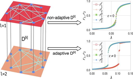
Figure 1. Schematic representation of the duplex network (l = 1, 2) having non-adaptive or adaptive inter-layer coupling between interconnected nodes. The non-adaptive case (learning rate ɛ = 0) leads to a continuous transition, whereas the Hebbian learning rule (ɛ ≠ 0) yields a discontinuous route to synchronization and then an irreversible route to desynchronization. rf and rb denote order parameter in the forward and backward continuation of coupling strength λ, respectively.
Download figure:
Standard image High-resolution image2. Model
Let us start with investigating how the Hebb's neural learning mechanism governing the inter-layer weight (strength) affects the phase transition in the multiplexed layers. In order to achieve this, we consider a multiplex network composed of two layers of the same size N. The dynamics of nodes in each layer is governed by the Kuramoto model [40]. The inter-layer link weight D[ii] between node i in a layer and its counterpart in the other layer is adaptive in nature. Hence, the evolution of the phase oscillators is governed by
where i = 1, ..., N, subscripts 1 and 2 stand for the two distinct layers, and λ represents intra-layer coupling strength, here λ1 = λ2 = λ. The instantaneous phase of the ith node is denoted by ![${\theta }_{l}^{\left[i\right]}\left(t\right)$](https://content.cld.iop.org/journals/1367-2630/22/12/122001/revision3/njpabcf6bieqn1.gif) and its natural frequency
and its natural frequency ![${\omega }_{l}^{\left[i\right]}$](https://content.cld.iop.org/journals/1367-2630/22/12/122001/revision3/njpabcf6bieqn2.gif) follows uniform or unimodal distribution g(ωl
). The intra-layer connectivity between the nodes following a network topology is encoded in the adjacency matrix Al
such that
follows uniform or unimodal distribution g(ωl
). The intra-layer connectivity between the nodes following a network topology is encoded in the adjacency matrix Al
such that ![${A}_{l}^{\left[ij\right]}=1\enspace \left(0\right)$](https://content.cld.iop.org/journals/1367-2630/22/12/122001/revision3/njpabcf6bieqn3.gif) if ith and jth nodes are connected (disconnected). The dynamically adaptive weight D[ii] of an inter-layer link between each pair of interconnected (mirror) nodes in the two layers is determined by the following Hebbian learning rule
if ith and jth nodes are connected (disconnected). The dynamically adaptive weight D[ii] of an inter-layer link between each pair of interconnected (mirror) nodes in the two layers is determined by the following Hebbian learning rule

where α ∈ [0, 1] is a factor which amplifies the amount of learning if the two nodes are synchronized and ɛ ∈ [0, 1] is the learning rate. The D[ii] in equation (2) prevents the inter-layer coupling weight from increasing or decreasing without bounds. Hence, the supra-adjacency matrix of the multiplex network is adaptive, and includes un-weighted intra-layer links and adaptive weighted inter-layer links:

where I is the identity matrix.
To track the level of coherence in the system, we define order parameter rl for a layer l in terms of the average phase ψl as

rl = 1 represents a completely synchronous state, while rl = 0 implies total incoherence. In a similar way, one can define global in-phase (one-cluster) order parameter for the entire multiplex network as

Furthermore, to capture the degree of global anti-phase (two-cluster) synchronization, a new global order parameter R2 (dipole moment of the distribution of anti-phases) [35, 41] is defined as follows

where
Here, R measures both the one-cluster and the two-cluster synchronization. Hence in order to determine the degree of two-cluster synchronization, the term R' is adjusted in equation (6) for one-cluster synchronization.
3. Results
We consider a multiplex network made of two different realizations of Erdös–Rényi (ER) random networks [42] having average intra-layer connectivity ⟨k1⟩ = ⟨k2⟩ = 10. The nodes in both layers are assigned different realizations of initial phases and natural frequencies drawn from a uniform random distribution such that θ[i] ∈ [0, 2π) and ω[i] ∈ [−γ, γ) where γ = 0.5 unless otherwise stated, respectively. The initial N values of D[ii](t) are selected as D[ii](t = 0) = d[i]/N, where d[i] is the number of inter-layer links a node in one layer can have with the nodes in other layer. Here we adopt the simplest form of a multilayer network, i.e. d[i] = 1, ∀ i.
First, we investigate the impact of the learning rate ɛ on intra-layer synchronization in the multiplexed layers. Figure 2 illustrates the behavior of the order parameter (for both forward and backward transitions) for the two layers as a function of coupling strength λ for different values of learning rate ɛ sustained with a fixed choice of learning factor α. It is found that the two layers undergo a first-order transition (ES) for different values of ɛ. It is also unveiled that the backward critical coupling strength  is independent of the rate ɛ. However, the forward critical coupling strength
  at first decreases with the increase in ɛ, then no further change is observed for higher values (0.5–1) of α. Hence slower learning rates ɛ yield slightly wider hysteresis.

Figure 2. Adaptive multiplexing leads to ES. Order parameter for forward and backward transitions ( and
and  ) for either multiplexed ER layer (since the two layers synchronize simultaneously) corresponding to α = 0.5 and different values of ɛ. The network parameters are N = 1000 and ⟨k⟩ = 10 and γ = 0.5.
Download figure:
Standard image High-resolution imageNext, the impact of the amplification factor α with a fixed choice of ɛ is reported in figure 3. The two layers follow a first-order transition with significantly different hysteresis width for different values of α. At very low α, a second-order transition is observed. With the increase in α, the forward critical  significantly increases while the backward critical coupling
  remains independent on α as well. Thus, each increase in α leads to a broader hysteresis width.

Figure 3. Impact of α: order parameters  (forward) and
  (backward) for the two multiplexed ER layers. ɛ = 0.1 and different values of α. Network parameters are the same as in the caption of figure 2.
Download figure:
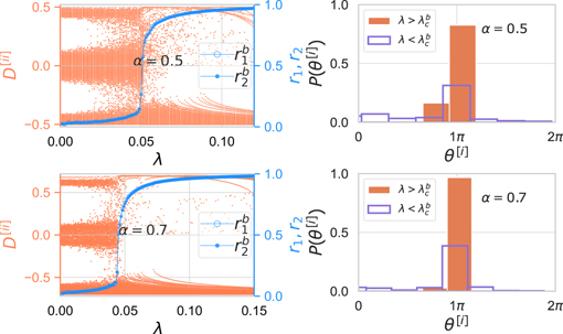
Standard image High-resolution imageTo gather information at a microscopic level on the origin of the first-order transition, we investigate the behavior of D[ii], the distribution P(Δθ[i]) of ![${\Delta}{\theta }^{\left[i\right]}=\vert {\theta }_{2}^{\left[i\right]}-{\theta }_{1}^{\left[i\right]}\vert $](https://content.cld.iop.org/journals/1367-2630/22/12/122001/revision3/njpabcf6bieqn12.gif) , global in-phase (R1) and anti-phase (R2) order parameter in figure 4. Note that the similar investigations are also presented for the case of
, global in-phase (R1) and anti-phase (R2) order parameter in figure 4. Note that the similar investigations are also presented for the case of ![${\omega }_{1}^{\left[i\right]}={\omega }_{2}^{\left[i\right]}$](https://content.cld.iop.org/journals/1367-2630/22/12/122001/revision3/njpabcf6bieqn13.gif) in appendix
in appendix  ), the inter-layer link population is mainly divided into two clusters of anti-weights, namely −α and α. Besides, there exists a neutral cluster around D[ii] → 0 containing a small fraction of link population, which increases with the decrease in the value of α. Interestingly, D[ii] and −D[ii] populations are almost equal in size. On the contrary, the inter-layer link population tends to converge to −α in the coherent state (
 ). The inter-layer link population having D[ii] → −α in the incoherent state originates a frustration at the respective interconnected end nodes. The triggered frustration at the end nodes of the inhibited (subjected to −α) inter-layer links curbs the formation of the largest synchronous cluster in their respective layers until a threshold for λ is reached. The larger the magnitude −α, the stronger the triggered frustration. Since a large value of −α imparts a stronger inhibition during the forward continuation of λ, a stronger and stronger λ is required for the abrupt formation of the largest synchronous cluster with each increase in α. Thus, the onset of first-order transition is witnessed at a larger forward critical coupling
  with each increase in α. For transition to desynchronization, the behavior of D[ii] when in synchronous and asynchronous state, is explained in appendix
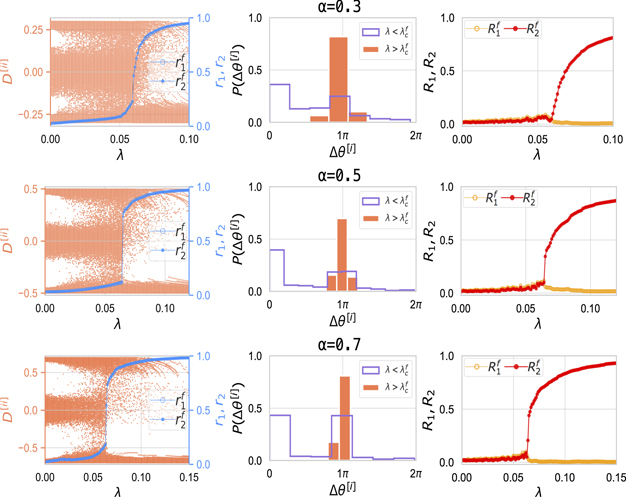
Figure 4. Mechanism behind ES D[ii] as a function of λ, the distribution P(Δθ[i]) of ![${\Delta}{\theta }^{\left[i\right]}=\vert {\theta }_{2}^{\left[i\right]}-{\theta }_{1}^{\left[i\right]}\vert $](https://content.cld.iop.org/journals/1367-2630/22/12/122001/revision3/njpabcf6bieqn17.gif) belonging to the incoherent and coherent state, and in-phase (R1) and anti-phase (R2) global order parameter as a function of λ for the multiplex network made of two ER layers. Results are produced for N = 1000 nodes, ɛ = 0.1 and γ = 0.5 and different values of α.
belonging to the incoherent and coherent state, and in-phase (R1) and anti-phase (R2) global order parameter as a function of λ for the multiplex network made of two ER layers. Results are produced for N = 1000 nodes, ɛ = 0.1 and γ = 0.5 and different values of α.
Download figure:
Standard image High-resolution imageIn the second column of figure 4, we study the distribution P(Δθ[i]) of ![${\Delta}{\theta }^{\left[i\right]}=\vert {\theta }_{2}^{\left[i\right]}-{\theta }_{1}^{\left[i\right]}\vert $](https://content.cld.iop.org/journals/1367-2630/22/12/122001/revision3/njpabcf6bieqn18.gif) , the difference between phases of the interconnected nodes for different values of α while keeping ɛ fixed. It unveils that in the incoherent state (
, the difference between phases of the interconnected nodes for different values of α while keeping ɛ fixed. It unveils that in the incoherent state ( ) belonging to an intermediate or higher value of α, two phase-clusters in each layer exist: one corresponding to
 ![${\theta }_{2}^{\left[i\right]}={\theta }_{1}^{\left[i\right]}$](https://content.cld.iop.org/journals/1367-2630/22/12/122001/revision3/njpabcf6bieqn20.gif) and the other to
and the other to ![$\vert {\theta }_{2}^{\left[i\right]}-{\theta }_{1}^{\left[i\right]}\vert =\pi $](https://content.cld.iop.org/journals/1367-2630/22/12/122001/revision3/njpabcf6bieqn21.gif) . In addition, the neutral cluster population remains distributed between these two clusters, whose population increases with the decrease in α. Hence, each multiplexed layer stays in a bi-clusters state in the incoherent state. Nevertheless, the P(θ[i]) in the coherent state (
. In addition, the neutral cluster population remains distributed between these two clusters, whose population increases with the decrease in α. Hence, each multiplexed layer stays in a bi-clusters state in the incoherent state. Nevertheless, the P(θ[i]) in the coherent state ( ) unveils a sharp single peaked (unimodal) distribution centered at
 ![$\vert {\theta }_{2}^{\left[i\right]}-{\theta }_{1}^{\left[i\right]}\vert =\pi $](https://content.cld.iop.org/journals/1367-2630/22/12/122001/revision3/njpabcf6bieqn23.gif) for any value of α. It implies that both layers are locked to two different phases at a mutual difference of π, i.e., the multiplex network comprises two anti-phase layers in the coherent state. As for the desynchronization transition, appendix
for any value of α. It implies that both layers are locked to two different phases at a mutual difference of π, i.e., the multiplex network comprises two anti-phase layers in the coherent state. As for the desynchronization transition, appendix
The third column of figure 4 illustrates R1 (equation (5)) and R2 (equation (6)) for different values of α. In the incoherent state one has that R1 → 0 and R2 → 0, as there exists two anti-phase clusters with θ[i] = 0 and θ[i] = π in each layer. In the coherent state, however, there exists a single cluster centered at θ[i] = π, hence still one has R1 → 0, while R2 displays an abrupt jump at the critical coupling strength. The height of the abrupt jump for R2 increases as α increases.
Now, since ![${\dot {D}}^{\left[ii\right]}=0$](https://content.cld.iop.org/journals/1367-2630/22/12/122001/revision3/njpabcf6bieqn24.gif) (from equation (2)) in the stationary state, one obtains (for ɛ ≠ 0)
(from equation (2)) in the stationary state, one obtains (for ɛ ≠ 0)

Further, it is revealed from figure 4 that for any value of α, there exists one-cluster coherent state in each layer obeying ![$\vert {\theta }_{2}^{\left[i\right]}-{\theta }_{1}^{\left[i\right]}\vert \simeq \pi $](https://content.cld.iop.org/journals/1367-2630/22/12/122001/revision3/njpabcf6bieqn25.gif) , hence D[ii] ≃ −α from equation (7). Also, there exists two populations of inter-layer anti-weights D[ii] ≃ α and D[ii] ≃ −α in the incoherent state, hence equation (7) yields
, hence D[ii] ≃ −α from equation (7). Also, there exists two populations of inter-layer anti-weights D[ii] ≃ α and D[ii] ≃ −α in the incoherent state, hence equation (7) yields ![$\vert {\theta }_{2}^{\left[i\right]}-{\theta }_{1}^{\left[i\right]}\vert =\mathrm{arccos}\left({\pm}1\right)=0,\pi $](https://content.cld.iop.org/journals/1367-2630/22/12/122001/revision3/njpabcf6bieqn26.gif) . Hence, the existence of the inhibitory D[ii] ≃ −α gives rise to anti-phase mirror-populations in the two layers in both incoherent and coherent states.
. Hence, the existence of the inhibitory D[ii] ≃ −α gives rise to anti-phase mirror-populations in the two layers in both incoherent and coherent states.
Phase diagrams: the data shown in figure 2 highlight the fact that any ɛ ≠ 0 is capable of inducing a first-order transition in the system and there exists a marginal difference in the critical coupling strength  for different values of ɛ. Figure 5 reports on how the hysteresis width
  varies in the α − λ space for different values of ɛ and for multiplexes composed of two homogeneous (ER–ER) and by one homogeneous (ER) and one heterogeneous (Barabási–Albert (BA) [43]) networks. There are systems in which the first-order transition arises without hysteresis, i.e.,
  as well [21, 44]. Nevertheless, in our case the first-order transition arises exhibiting a good hysteresis width complementing the abrupt jump, which gradually decreases in size as α reduces from 1 to a lower value. A further decrement in α gradually switches the route of transition from a discontinuous to a continuous one with a decrease in the abrupt jump size as well as the hysteresis width. For a better subtlety, the phase plots in figure 5 are simulated for an increment and a decrement in λ of Δλ = 0.002, and an increment in α of Δα = 0.02.
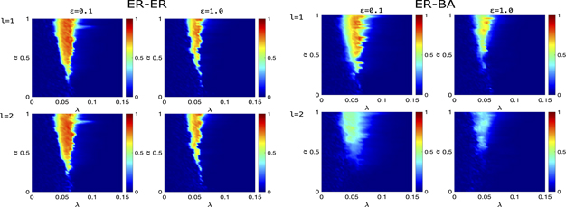
Figure 5. Phase diagrams α − λ of hysteresis width  , where l ∈ [1, 2], corresponding to two different values of ɛ (N = 1000, γ = 0.5). Data refers to pairs of a variety of network topology, namely ER–ER and ER–BA. Note that layer l = 2 denotes BA network for ER–BA configuration.
Download figure:
Standard image High-resolution imageThe ER–ER configuration exhibits a first-order transition for intermediate and higher values of α. Also, the associated hysteresis width for both the layers increases with an increase in α. Besides, a slower rate ɛ yields a wider hysteresis width for a given value of α as compared to the faster rate ɛ. For the ER–BA configuration, a rather weak hysteresis is observed for the ER layer in the range α = 0.5–1, while the BA layer does not feature a first-order transition route to synchronization because of the heterogeneity in degrees. For the same reason, a BA-BA configuration of multiplexes features a continuous route to synchronization for any value of α and ɛ.
4. Analytical treatment
To obtain an analytical expression for the order parameter, we take into account, for simplicity, a multiplex network consisting of two globally-connected (GC) layers l ∈ [1, 2] so that ![${A}_{l}^{\left[i,i\right]}=1/N$](https://content.cld.iop.org/journals/1367-2630/22/12/122001/revision3/njpabcf6bieqn31.gif) in model equation (1) and the order parameter defined in equation (4) for a complex network can then be expressed for a GC layer as following
in model equation (1) and the order parameter defined in equation (4) for a complex network can then be expressed for a GC layer as following

Note that the intrinsic frequencies of the nodes in both GC layers are selected from a uniform distribution ![${\omega }_{l}^{\left[i\right]}=-\gamma +\frac{\gamma }{N}\left(2i-1\right)$](https://content.cld.iop.org/journals/1367-2630/22/12/122001/revision3/njpabcf6bieqn32.gif) in the interval [−γ, γ] [44, 45]. Now equation (1) can be rewritten in the mean-field form using equation (8) as
in the interval [−γ, γ] [44, 45]. Now equation (1) can be rewritten in the mean-field form using equation (8) as

In the stationary state ![${\dot {D}}^{\left[ii\right]}=0$](https://content.cld.iop.org/journals/1367-2630/22/12/122001/revision3/njpabcf6bieqn33.gif) , for ɛ ≠ 0, thereby equation (2) leads to
, for ɛ ≠ 0, thereby equation (2) leads to

Hence, evolution of the nodes in the stationary state is ruled by the following self-consistent equations

Next, we gather from numerical simulations (see figure 5) that the distribution P(Δθ[i]) of ![${\Delta}{\theta }^{\left[i\right]}=\vert {\theta }_{2}^{\left[i\right]}-{\theta }_{1}^{\left[i\right]}\vert $](https://content.cld.iop.org/journals/1367-2630/22/12/122001/revision3/njpabcf6bieqn34.gif) for the two GC layers in the coherent state (
for the two GC layers in the coherent state ( ) follows a peaked (unimodal) distribution with its mean at 0 and standard deviation Δθ(λ). Therefore, the inter-layer term in the stationary state can be expressed as
  , and the model equation (9) can be rewritten as

In this way, stationary σ = σ(α, λ) accounts for the maximum possible inter-layer contribution in the evolution of phases in either layers. When the phases in each layer are locked to their respective mean-fields ![${\dot {\theta }}_{1}^{\left[i\right]}={{\Omega}}_{1}$](https://content.cld.iop.org/journals/1367-2630/22/12/122001/revision3/njpabcf6bieqn37.gif) and
and ![${\dot {\theta }}_{2}^{\left[i\right]}={{\Omega}}_{2}$](https://content.cld.iop.org/journals/1367-2630/22/12/122001/revision3/njpabcf6bieqn38.gif) , i.e.,
, i.e., ![$\vert {\omega }_{1}^{\left[i\right]}\vert -{{\Omega}}_{1}+\sigma {\leqslant}\lambda {r}_{1}$](https://content.cld.iop.org/journals/1367-2630/22/12/122001/revision3/njpabcf6bieqn39.gif) and
and ![$\vert {\omega }_{2}^{\left[i\right]}\vert -{{\Omega}}_{2}-\sigma {\leqslant}\lambda {r}_{2}$](https://content.cld.iop.org/journals/1367-2630/22/12/122001/revision3/njpabcf6bieqn40.gif) . Hence, one obtains
. Hence, one obtains ![$\mathrm{sin}\left({\theta }_{l}^{\left[i\right]}-{\psi }_{l}\right)=\frac{{\omega }_{l}^{\left[i\right]}-{{\Omega}}_{l}{\pm}\sigma }{\lambda {r}_{l}}$](https://content.cld.iop.org/journals/1367-2630/22/12/122001/revision3/njpabcf6bieqn41.gif) , which leads to the following set of the conditions (referred as CondI) to be satisfied simultaneously by the locked oscillators contributing to rl
;
, which leads to the following set of the conditions (referred as CondI) to be satisfied simultaneously by the locked oscillators contributing to rl
;
CondI:
The order parameter in equation (8) for the phase-locked oscillators can be expressed as

which can be further simplified as
Now, Δθ → 0 (Δθ ≃ 0.002–0.003) for any  corresponding to locked state, hence σ → 0 (see figure 6).

Figure 6. Matching with analytical predictions: order parameter for a multiplex network comprising two GC layers (N = 10 000 nodes) for ɛ = 0.1 and ![${\omega }_{1}^{\left[i\right]}={\omega }_{2}^{\left[i\right]}$](https://content.cld.iop.org/journals/1367-2630/22/12/122001/revision3/njpabcf6bieqn43.gif) ; γ = 1. Numerical estimations for backward transition for different values of α, and their analytical predictions given by equations (16), (18) and (21).
; γ = 1. Numerical estimations for backward transition for different values of α, and their analytical predictions given by equations (16), (18) and (21).
Download figure:
Standard image High-resolution imageBackward critical coupling: in the continuum limit N → ∞, the order parameter can be rewritten in its integral form

For a uniform distribution  for |ωl
| < γ and since Ωl
→ 0, the order parameter in equation (15) reduces to
for |ωl
| < γ and since Ωl
→ 0, the order parameter in equation (15) reduces to

If Δθ[i] ∼ π for the pairs of oscillators locked in their respective layers, then σ → 0. In such a scenario, we in principal reach to the single layer case for the oscillators locked in their respective layers, thus the order parameter turns into the following:

For λrl
= γ, equation (17) yields  . Hence, the backward critical coupling strength is given by

Forward critical coupling: from equation (11), the contribution from inter-layer coupling yields bounds (maximal or minimal) of ±α/2. Moreover, in the incoherent state at  (rl
= 0), the contribution from intra-layer mean-field is negligible. Hence, the evolution of the nodes at
(rl
= 0), the contribution from intra-layer mean-field is negligible. Hence, the evolution of the nodes at  is driven entirely by the effective critical frequency

So, the critical frequencies at  are bounded in the effective interval
 ![${\omega }_{l\mathrm{c}}^{\left[i\right]}\in \left(-\gamma -\alpha /2,\gamma +\alpha /2\right)$](https://content.cld.iop.org/journals/1367-2630/22/12/122001/revision3/njpabcf6bieqn49.gif) . Hence, the dynamics of the nodes at
. Hence, the dynamics of the nodes at  can be approximated as

Next, following the same methodology adopted for the backward transition, the forward critical threshold is given by

In figure 6, numerical results for the order parameter and the forward and backward thresholds for either GC layers (since both the GC layers synchronizes simultaneously) and their analytical predictions given by equations (16), (18) and (21), are shown for different values of α when  = 0.1. The analytical predictions match fairly well with their numerical estimations. From theoretical and numerical outcomes we deduce that the threshold for first-order de-synchronization does not depend on either α or ɛ, however the threshold for the onset of first-order transition to synchronization does depend on α. Further, we show the dependence of
  and
and  on factor α both numerically as well as analytically as shown in figure 7. The α − λ phase plot unveils that
  remains independent of α and fixed to
  . However,
  does show dependence on α closely following equation (21).
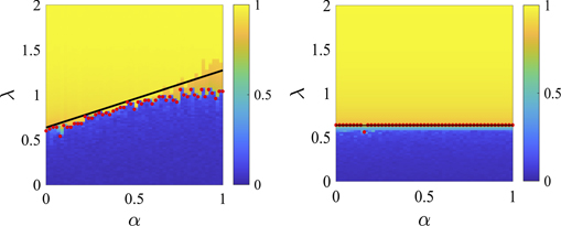
Figure 7.
α dependence of  :
:  and
and  (for either layer) as a function of factor α for two GC layers with ɛ = 0.1 and
 ![${\omega }_{1}^{\left[i\right]}={\omega }_{2}^{\left[i\right]}$](https://content.cld.iop.org/journals/1367-2630/22/12/122001/revision3/njpabcf6bieqn59.gif) ; γ = 0.5. Red circle indicates numerical assessment for
; γ = 0.5. Red circle indicates numerical assessment for  (left panel) and
  (right panel) while black solid line denotes their analytical prediction from equations (18) and (21).
Download figure:
Standard image High-resolution image5. Robustness against network size N and structure
We explored the phenomena of ES as a consequence of adaptive multiplexing for larger size as well as for different network architecture. Numerical results for larger sizes N = 10 000 of multiplex networks composed of two different pairs of homogeneous topology, namely ER–ER and GC–GC network are shown in figure 8. Numerical results for the order parameter corresponding to different values of α for large size N are consistent with those obtained for rather small network size N = 1 000. Hence, the occurrence of ES as an outcome of inter-layer adaptation is robust against networks size N and homogeneous network topology of the multiplex network. Nevertheless, the employed inter-layer Hebbian adaptive mechanism is incapable in triggering ES transition in heterogeneous topology for a multiplexed layer as can be observed for BA layer in the phase plots for ER–BA multiplex configuration in figure 5.
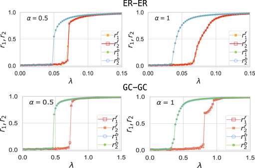
Figure 8. For larger size networks: synchronization profile (rl
− λ) for larger network size (N = 10 000) of multiplexed ER–ER layers and GC–GC layers. Other parameters are ⟨k1⟩ = ⟨k2⟩ = 10, = 0.1 and γ = 0.5.
Download figure:
Standard image High-resolution image6. Effect of different average connectivity ⟨k⟩
So far we have examined the behavior of phase transition for the same average connectivity for the two multiplexed layers. Here we examine the nature of phase transition for multiplex networks with contrasting average connectivity for the two ER layers. Figure 9 exhibits the behavior of order parameter when ⟨k1⟩ is kept fixed to 10 while ⟨k2⟩ is tested with different values of average degree. In figure 9(a), the two ER layers with ⟨k1⟩ = ⟨k2⟩ = 10 synchronize and de-synchronize abruptly and simultaneously at the same critical threshold. However in figure 9(b), the layer with contrasting ⟨k2⟩ = 20 abruptly synchronizes relatively at a lower forward threshold  , because of a large number of intra-layer connections, as compared to the threshold
  of layer with ⟨k1⟩ = 10. Now even higher ⟨k2⟩ = 30 sets the onset of transition at further lower threshold
  . Moreover, abrupt de-synchronization of the two layers takes place at the same critical threshold
  . Not only that both
  and
and  for the two layers shift towards lower values with each increasing difference in ⟨k1⟩ and ⟨k2⟩. Hence, contrasting average connectivities of the layers set the onset of ES transition at lower threshold.

Figure 9. For different average degree: synchronization profile (r − λ) of multiplexed ER–ER layers with different average degrees, i.e., ⟨k1⟩ = 10 while (a) ⟨k2⟩ = 10, (b) ⟨k2⟩ = 20, and (c) ⟨k2⟩ = 30. Simulations are presented for = 0.1, α = 0.5 and γ = 0.5.
Download figure:
Standard image High-resolution image7. Conclusion
We studied the adaptive evolution of connection weights of inter-layer links in multiplex networks. The connection weight between a pair of interconnected nodes is strengthened if they are in phase. Such an Hebbian learning rule plays an important role in shaping the dynamics of the phases, as well as interlayer links control, in turn, intra-layer synchronization. In the asynchronous state of both the layers, the existing Hebbian learning adaptation segregates the interlayer link population into two almost equal groups of excitatory and inhibitory weights. The half population of inhibitory (excitatory) weights makes their respective end mirror nodes anti-phase (in-phase) in the two layers. It is for the half inhibitory weight population, which causes the frustration among the nodes in the two layers and leads to a first-order transition route to synchronization. In the synchronous state of the two layers, the Hebbian learning adaptation drives the entire interlayer link population to form a global cluster of inhibitory weights, which yields two anti-phase layers. Thus the interlayer Hebbian plasticity not only triggers the first-order transition but also provides a great amount of control over the abruptness and area of the associated hysteresis loop by means of the Hebbian learning parameters. The same has been conveyed through the phase diagrams presenting hysteresis width for multiplex networks with different combinations of topology. It has also been demonstrated theoretically as well as numerically that the backward critical coupling strength is independent of both the learning parameters, while the forward critical coupling strength is shown to have explicit dependence on the learning parameters. However, the proposed Hebbian plasticity based scheme is capable of bringing about the first-order transition in only homogeneous multiplexed layers.
Acknowledgments
SJ thanks CSIR grant 25(0293)/18/EMR-II for financial support. ADK acknowledges Govt of India CSIR grant 25(0293)/18/EMR-II for RA fellowship.
Appendix A.:
![${\omega }_{1}^{\left[i\right]}={\omega }_{2}^{\left[i\right]}$](data:image/png;base64,iVBORw0KGgoAAAANSUhEUgAAAAEAAAABCAQAAAC1HAwCAAAAC0lEQVR42mNkYAAAAAYAAjCB0C8AAAAASUVORK5CYII=) case
case
![${\omega }_{1}^{\left[i\right]}={\omega }_{2}^{\left[i\right]}$](https://content.cld.iop.org/journals/1367-2630/22/12/122001/revision3/njpabcf6bieqn68.gif)
The microscopic dynamics behind the origin of ES is simplified further when taking into account ![${\omega }_{1}^{\left[i\right]}={\omega }_{2}^{\left[i\right]}$](https://content.cld.iop.org/journals/1367-2630/22/12/122001/revision3/njpabcf6bieqn69.gif) for multiplex networks made of two ER layers. The first column in figure A1 shows the absence of neutral cluster around D[ii] → 0 which is present for the case of
for multiplex networks made of two ER layers. The first column in figure A1 shows the absence of neutral cluster around D[ii] → 0 which is present for the case of ![${\omega }_{1}^{\left[i\right]}\ne {\omega }_{2}^{\left[i\right]}$](https://content.cld.iop.org/journals/1367-2630/22/12/122001/revision3/njpabcf6bieqn70.gif) , hence the identical frequencies of the interconnected nodes leads to only two pure anti-weight states, namely D[ii] ≃ α and D[ii] ≃ −α. And for that matter, only two equal sized clusters are obtained following
, hence the identical frequencies of the interconnected nodes leads to only two pure anti-weight states, namely D[ii] ≃ α and D[ii] ≃ −α. And for that matter, only two equal sized clusters are obtained following ![$\vert {\theta }_{2}^{\left[i\right]}-{\theta }_{1}^{\left[i\right]}\vert =0$](https://content.cld.iop.org/journals/1367-2630/22/12/122001/revision3/njpabcf6bieqn71.gif) and π in the incoherent state (see second column). Anyhow, one single peak is obtained in the coherent state. In the third column, the behavior of the final states of D[ii] against Δθ[i] affirms the fact that for any α in the coherent state, a single phase-cluster with
and π in the incoherent state (see second column). Anyhow, one single peak is obtained in the coherent state. In the third column, the behavior of the final states of D[ii] against Δθ[i] affirms the fact that for any α in the coherent state, a single phase-cluster with ![$\vert {\theta }_{2}^{\left[i\right]}-{\theta }_{1}^{\left[i\right]}\vert =\pi $](https://content.cld.iop.org/journals/1367-2630/22/12/122001/revision3/njpabcf6bieqn72.gif) originates from the cloud of D[ii] → −α. In the incoherent state, one-half population of the inter-layer link experiencing D[ii] → α gives birth to a phase-cluster with
originates from the cloud of D[ii] → −α. In the incoherent state, one-half population of the inter-layer link experiencing D[ii] → α gives birth to a phase-cluster with ![${\theta }_{2}^{\left[i\right]}={\theta }_{1}^{\left[i\right]}$](https://content.cld.iop.org/journals/1367-2630/22/12/122001/revision3/njpabcf6bieqn73.gif) in each layer while the other-half population experiencing −α leads to phase-cluster with
in each layer while the other-half population experiencing −α leads to phase-cluster with ![$\vert {\theta }_{2}^{\left[i\right]}-{\theta }_{1}^{\left[i\right]}\vert =\pi $](https://content.cld.iop.org/journals/1367-2630/22/12/122001/revision3/njpabcf6bieqn74.gif) in each layer. The fourth column infers that the abrupt jump in R2 at the onset of synchronization shows the existence of anti-phase layers. Also, the special case of
in each layer. The fourth column infers that the abrupt jump in R2 at the onset of synchronization shows the existence of anti-phase layers. Also, the special case of ![${\omega }_{1}^{\left[i\right]}={\omega }_{2}^{\left[i\right]}$](https://content.cld.iop.org/journals/1367-2630/22/12/122001/revision3/njpabcf6bieqn75.gif) shows a handsome jump size in R2 for any value of α as that for the case of
shows a handsome jump size in R2 for any value of α as that for the case of ![${\omega }_{1}^{\left[i\right]}\ne {\omega }_{2}^{\left[i\right]}$](https://content.cld.iop.org/journals/1367-2630/22/12/122001/revision3/njpabcf6bieqn76.gif) .
.

Figure A1. Mechanism behind ES for ![${\omega }_{1}^{\left[i\right]}={\omega }_{2}^{\left[i\right]}$](https://content.cld.iop.org/journals/1367-2630/22/12/122001/revision3/njpabcf6bieqn77.gif) : D[ii] as a function of λ, P(Δθ[i]) of
: D[ii] as a function of λ, P(Δθ[i]) of ![${\Delta}{\theta }^{\left[i\right]}=\vert {\theta }_{2}^{\left[i\right]}-{\theta }_{1}^{\left[i\right]}\vert $](https://content.cld.iop.org/journals/1367-2630/22/12/122001/revision3/njpabcf6bieqn78.gif) belonging to the incoherent and coherent state, D[ii] against Δθ[i], and R1 and R2 order parameter as a function of λ for the multiplex network comprising two ER layers. Results are produced for N = 1000 nodes, ɛ = 0.1 and γ = 0.5 and different values of α.
belonging to the incoherent and coherent state, D[ii] against Δθ[i], and R1 and R2 order parameter as a function of λ for the multiplex network comprising two ER layers. Results are produced for N = 1000 nodes, ɛ = 0.1 and γ = 0.5 and different values of α.
Download figure:
Standard image High-resolution imageAppendix B.: Weight and phase distribution in backward continuation
Figure B1 illustrates the behavior of stationary values of D[ii] as a function of λ, and the distribution P(Δθ[i]) for different values of α in the backward continuation. Beginning with a synchronous state the distribution P(Δθ[i]) sports a unimodal distribution centered at π, and even after abrupt desynchronization it tends to follow unimodal distribution with its mean still at π but sporting relatively a shorter peak and broader deviation. In both the asynchronous and synchronous state, a large population of interlayer links has D[ii] → −α. However the fraction of interlayer links favoring D[ii] → α is less and varies depending on the value of λ. It is approximately less than 10% and 1% of number of interlayer links in the asynchronous and synchronous state, respectively.
Figure B1.
D[ii] and P(Δθ[i]) in backward continuation: D[ii] as a function of λ, P(Δθ[i]) of ![${\Delta}{\theta }^{\left[i\right]}=\vert {\theta }_{2}^{\left[i\right]}-{\theta }_{1}^{\left[i\right]}\vert $](https://content.cld.iop.org/journals/1367-2630/22/12/122001/revision3/njpabcf6bieqn79.gif) belonging to the incoherent and coherent state in the backward continuation of λ. Results are generated for multiplex network composed of two ER layers with N = 1000 nodes, ɛ = 0.1 and γ = 0.5.
belonging to the incoherent and coherent state in the backward continuation of λ. Results are generated for multiplex network composed of two ER layers with N = 1000 nodes, ɛ = 0.1 and γ = 0.5.
Download figure:
Standard image High-resolution image