


Abstract
A single chirped few-femtosecond pulse can be used to control and image coupled electron-nuclear dynamics. Using full ab initio simulations of the simplest molecule,  as a prototype target, we show that for intermediate values of the chirp, interference between sequential and direct contributions enables significant control over ionization yields, even when taking into account the effective decoherence introduced by nuclear motion and the presence of an electronic continuum. For larger values of the chirp, the single chirped pulse reproduces a classical pump–probe setup, with the chirp parameter mapping an effective time delay between the pumping and probing frequencies of the pulse. After demonstrating this numerically, we present a full analytical solution for the two-photon ionization amplitudes that provides an intuitive analogy between the molecular dynamics induced by a single chirped pulse and a traditional pump–probe setup.
Export citation and abstract BibTeX RIS

Original content from this work may be used under the terms of the Creative Commons Attribution 3.0 licence. Any further distribution of this work must maintain attribution to the author(s) and the title of the work, journal citation and DOI.
1. Introduction
Attosecond science aims to dynamically modify light–matter response at the electronic level acting at its intrinsic time scale of motion [1, 2]. In pursuing this goal, worldwide efforts to improve sources of ultrashort light pulses have made possible the generation of attosecond-scale x-ray and XUV pulses using free-electron lasers (FELs) [3] and high-order harmonic generation techniques [4–6]. These sources are nowadays capable of providing bright and intense pulses with a high degree of coherence in order to image and even guide electron motion on its natural time scale in atoms and molecules [7]. One of the most successful strategies to track electron dynamics to date uses a pump–probe setup combining an attosecond x-ray or XUV pulse to excite or ionize the system, followed by a femtosecond IR probe to retrieve an image of electronic processes in time or to drive the reaction [8, 9]. Recent experiments at the Linac Coherent Light Source FEL have demonstrated coherent control over the ultrafast Coulomb explosion of  using x-ray and IR pulses [10]. Similar experiments combining x-rays with optical-frequency pulses were also successfully performed to explore ultrafast dynamics in more complex molecular targets [11, 12]. The key to access electron dynamics is the availability of attosecond time resolution in these schemes, rather than the production of ultrashort pulses. This has been proven, for instance, in experiments performed at FERMI that have demonstrated how phase-controlled femtosecond pulses (few tens of femtoseconds) in a two-color scheme can achieve control and chemical specificity with temporal resolution as short as 3 as [13].
In typical experiments, attosecond pulses are not produced with a flat spectral phase (i.e. as transform-limited pulses), but have an intrinsic chirp such that different frequencies within the pulse arrive at different times. This chirp can be characterized and manipulated using dispersive optical elements [14, 15], with most existing applications using dispersion compensation in order to generate transform-limited pulses. However, by controlling the relative arrival times of different frequencies, the chirp could also be used as a control knob to achieve sub-femtosecond time-resolved images and control of electron dynamics. Earlier theoretical and experimental works in atoms established that two-photon absorption rates could be manipulated by modifying the spectral phase of an exciting femtosecond laser pulse, but with the maximum yield always corresponding to transform-limited pulses [16]. However, subsequent investigations, also using atomic targets, showed that the presence of resonant states can break this limit and that controlling the spectral phases allows one to attain larger two-photon excitation rates even though the peak intensity decreases [17]. These findings raised the question of whether transform-limited pulses are a prerequisite for attosecond science. A theoretical model applied to a two-level system already showed that an attosecond pump–probe setup using chirped pulses can provide the same temporal resolution as a scheme using transform-limited pulses [18]. More recent simulations in atoms using second-order perturbation theory have captured the carrier-envelope phase and chirp dependencies of electron angular distributions upon multiphoton ionization of an atom with a single pulse [19, 20], thus demonstrating a certain degree of control over electron motion. Analogous applications in molecules could open new avenues to manipulate the outcome of chemical reactions, but face the challenge of dealing with nuclear motion coupled to electronic dynamical processes. Chemical reaction control has already been demonstrated by employing intense femtosecond IR pulses [21, 22] distorting the molecular potential. More recent studies have shown that by chirping these intense IR fields, it is possible to achieve quantum control of molecular photodissociation of the hydrogen molecular ion [23, 24]. However, we here focus on control schemes where the molecular potential remains unaffected, i.e. on an approach similar to previous experiments using chirped femtosecond pulses with optical frequencies to manipulate multiphoton excitation and ionization of molecules [25, 26]. We recently demonstrated that a single chirped UV pulse can be employed to retrieve time-resolved images of molecular wave packets with attosecond resolution, providing an alternative to the long-awaited UV-pump/UV-probe attosecond schemes [27]. In the current manuscript, we expand on this idea and show that chirped attosecond pulses provide a versatile tool to both probe and control coupled electron-nuclear dynamics in molecules. Specifically, we provide a detailed analysis of chirped-pulse and nuclear decoherence effects in ultrafast molecular processes triggered in the simplest molecule, the hydrogen molecular ion  We will discuss the use of a simple sequential approximation, and its connection to the formally exact time-dependent perturbation theory expressions, to model the action of the single pulse as a pump and probe tool. The hydrogen molecular ion provides a benchmark target to investigate correlated electron-nuclear motion, as it allows for a full-dimensional quantum mechanical treatment beyond the Born–Oppenheimer approximation within current computational capabilities.
The manuscript is organized as follows. In section 2, we first introduce our numerical implementation to describe the ultrafast dynamics induced in the hydrogen molecular ion by using ultrafast chirped pulses. We then discuss time-dependent perturbation theory, which allows us to obtain closed-form expressions for two-photon ionization amplitudes within the perturbative limit. Section 3 discusses the effect of nuclear motion on chirp-controlled total ionization yields. We first treat the molecule within the fixed-nuclei approximation, in which it effectively behaves like an atom. Even within this limit, we find significant differences between photoionization, in which the final states present a continuum, and excitation to a single well-defined state. We then treat nuclear motion during the pulse and explicitly show how this washes out most of the coherence effects found for fixed nuclei, at least when looking at integrated quantities such as the total ionization-dissociation yield. In section 4, we study energy-resolved observables, focusing on the dynamical aspects, i.e. the wave-packet motion encoded in the final ionization amplitudes. We demonstrate how to retrieve attosecond time-resolved images by tracing energy-differential ionization yields and provide the formal derivation of the analytical expressions to compute the amplitudes within the time-dependent second order perturbation theory assuming Gaussian-shaped finite pulses.
2. Methodology
2.1. Time-dependent Schrödinger equation (TDSE)
The time-dependent wave function Φ(t, r, R) that describes the molecular system subject to pulsed radiation is solution of the TDSE

where r and R stand for the electronic and nuclear coordinates, respectively, and t is the time. We use atomic units unless otherwise stated. The theoretical description of the hydrogen molecular ion has been achieved in previous works employing cylindrical [28, 29] or prolate spheroidal coordinates [30–34]. For the numerical respresentation of the molecular wave function, we here employ a single-center expansion using spherical harmonics,  to treat the angular degrees of freedom of the electron and a discrete variable representation combined with a finite element method (DVR) for the radial part of both the electronic (ϕi(r)) and nuclear (χj(R)) components of the wave packet. However, different from our previously employed spectral methods using a single-center expasion [35, 36], in order to represent the coupled electron-nuclear dynamics, we now use a direct basis expansion of the wave function without relying on the Born–Oppenheimer (adiabatic) approximation, such that non-adiabatic couplings are implicitly included. We restrict the present work to fixed-in-space molecules, such that we can omit the rotational motion of the nuclei, and the expansion for the time-dependent wave function reads:

The full Hamiltonian, H(t), can be written as the sum of a time-independent Hamiltonian describing the isolated molecule and a time-varying potential induced by the laser pulse, H(t) = H0 + V(t). The light interaction term, V(t), is treated within the dipole approximation, which neglects the spatial dependence of the electromagnetic field over the size of the molecule. This approximation remains valid for the wavelength range within the XUV region here employed. The laser-molecule term can thus be written, in the length gauge, as the product of the electronic coordinates and the electric field,  In order to test numerical convergence of the method [37], we have checked that simulations within the velocity gauge, where the interaction term is given by the electronic momentum and the vector potential of the pulse, V(t) = p · A(t), give the same results as in length gauge for the basis sets employed here. The expressions that define the electromagnetic field corresponding to a frequency-chirped pulse are provided in section 2.3 together with a time-frequency analysis. After the action of the radiation source, the resulting scattering wave function that defines the final quantum state of the molecule at a given energy E is calculated from the time-propagated wave packet by solving the time-independent Schrödinger equation using a exterior complex scaling of both the electronic and nuclear coordinates to impose the outgoing boundary conditions that define the half-collision problem [38]

where H0 is the Hamiltonian of the molecule in the absence of external field. The extraction of the ionization amplitudes, total and differential in energy sharing and ejection angles for protons and electrons, can be achieved by employing a surface integral formalism as described in previous works for the three-body break-up problem in atoms [38, 39]. A thorough description of this numerical approach, including the technical implementation employing open-source SLEPc libraries for the diagonalization procedures [40, 41], and computational details, is provided elsewhere [37].
2.2. Time-dependent perturbation theory
For the description of a two-photon process resulting from the interaction with a relatively low-intensity laser pulse, an alternative to the direct solution of the TDSE is the use of second-order time-dependent perturbation theory, with the corresponding molecular wave packet  given by:


where  is the ground (or initially prepared) state of the molecule with energy ωg.
  is the driving operator in the interaction picture,
  with V(t) in velocity or length gauge as previously defined. The ionization amplitude corresponding to a final scattering state
  with total vibronic energy Ef is obtained by projecting it into the second order molecular wave packet

which explicitly results in a double integral in time and a sum over all the vibronic eigenstates (m) of the target

where Δωmg = ωm − ωg, Δωfm = ωf − ωm, and ωm is the energy of state m. μ stands for the corresponding dipole operator and F(t) for the electric field E(t) or vector potential A(t), depending on the gauge of choice. For some specific pulse shapes (such as Gaussian pulses), this double integral in time can be performed analytically even with chirped pulses to obtain an expression that separates the result into a 'shape function' that only depends on the involved frequencies, and target-dependent products of dipole transition moments, as it is formally demonstrated in section 4 of the present manuscript. For the wavelengths and laser intensities here employed, we have checked that the computed full-dimensional molecular wave packets and amplitudes are identical within TDPT and by solving the TDSE. The use of TDPT, as we show in the following sections, is particularly convenient to truncate our simulations and to establish simple models to gain deeper insights on the underlying physical mechanisms that govern molecular dynamics.
2.3. Chirped pulses
The electromagnetic field E(t) of a chirped Gaussian pulse can be written as [18, 42, 43]

with maximum amplitude  a Gaussian envelope
  and assuming linearly polarized light. Here, η is the chirp parameter and the chirp-dependent pulse duration is given by
  The temporal phase is

with the corresponding instantaneous frequency ω(t) = dϕ(t)/dt changing linearly in time. Note that, for a more consistent definition with respect to the literature, the sign of η is reversed with respect to [27]. For unchirped pulses (η = 0), E0 is the peak field amplitude, T0 defines the duration of the pulse (FWHM of the field envelope is  ), and ω0 is the carrier frequency. For the given parametrization, adding a chirp (
 ) corresponds to stretching the same frequencies contained in the pulse over a longer duration, such that the duration of the pulse increases and the peak amplitude decreases. At the same time, the spectral density
  remains unchanged [44] (under the assumption that positive- and negative-frequency contributions do not overlap, i.e. that the pulse bandwidth does not extend to zero frequency), where


is the Fourier transform, with spectral phase given by

An illustration of the chirped pulses employed here is shown in figure 1. The left column shows the electromagnetic field as a function of time for up-chirped (panel a, η > 0), unchirped (b, η = 0) and down-chirped (c, η < 0) pulses. The reference transform-limited pulse, i.e. equation (7) evaluated at η = 0, is plotted in figure 1(b), and also (gray full line) in figures 1(a) and (c). The middle column panels, (d)–(f), of figure 1 show the squared amplitude and phase of their corresponding Fourier transform, where we can see that all pulses share the exact same energy distribution but with different quadratic (frequency-chirped) phase. Finally, in the rightmost column, figures 1(g)–(i), we plot the corresponding Wigner distributions, i.e. the time-frequency analysis [45, 46], for the most up-chirped pulse with η = 10 (panel (g)), the transform limited pulse with η = 0 (panel (h)) and the most down-chirped pulse with η = −10 (panel (i)). The Wigner distributions represent the frequency components of the pulse in time. Through these plots, we can easily see that for the unchirped pulse (panel (h)), all frequencies will simultaneously reach the molecular target. For the up-chirped pulses (panel (g)), the lower frequencies interact with the molecule at earlier times than the higher ones, while the opposite applies for the down-chirped pulses (panel (i)).

Figure 1. Left column: electromagnetic field as a function of time for up-chirped (a), unchirped (b) and down-chirped (c) pulses. The transform limited pulse ( ) is also included as a faint gray line in (a) and (c) for reference, and corresponds to an unchirped pulse of TFWHM = 450 as duration with 1.1 × 10¹³ W cm−2 of laser intensity and ω0 = 0.6 au of central frequency. Panel (a) shows the up-chirped pulses defined with η = 5 (red) and η = 10 (blue). Panel (b) shows the Fourier-transform limited pulse. Panel (c) shows the down-chirped pulses defined with η = −5 (red) and η = −10 (blue). Middle column: Fourier transform (amplitude and phase) of the electromagnetic fields on the left. Right column: Wigner distributions for the vector potential (time-frequency plots) for the pulses defined with η = 10 (g), η = 0 (h) and η = −10 (i).
Download figure:
Standard image High-resolution image3. Chirp-enhanced ionization yields
Manipulation of two-photon absorption rates by pulse shaping has been experimentally realized in atoms [16, 47] and crystals [48] using femtosecond IR pulses. There, a proper choice of the spectral phase favors two specific resonant transitions enhancing excitation into a particular state. In the current case of molecular photoionization using significantly shorter XUV pulses, the physical scenario is quite different. On the one hand, ionization implies a continuum of final electronic states, thus decreasing the energy selectivity of the second photon absorption with respect to excitation. On the other hand, molecules, and in particular light molecules, introduce the nuclear degrees of freedom as a source of additional broadening as well as decoherence. Consequently, the interference patterns previously described for atomic excitation [49], due to interference of a resonant and a non-resonant two-photon path, are strongly suppressed as we discuss in the present section. In addition, the use of broadband ultrashort pulses induces correlated dynamics of molecular wave packets containing a coherently populated manifold of vibrational and electronic states. This dynamics can be captured using chirped pulses, as we demonstrate in section 4.
We have previously demonstrated the possibility of manipulating two-photon molecular ionization using an attosecond chirped UV pulse [27]. We here focus on unraveling the underlying physics governing molecular dynamics triggered by chirped pulses in order to disentangle the role of electron and nuclear dynamics. We first work within the fixed-nuclei approximation, in which molecules behave similar to atoms, and investigate the two-photon single ionization yield of  Figure 2(a) shows a scheme of the ionization process: the
  molecule, initially in its ground state, interacts with an ultrashort pulse with a central frequency of ω0 = 0.6 au, between the two lowest excited states of the molecule. At this frequency, ionization only occurs after two-photon absorption. The ionization yield is plotted in figure 2(b) as a function of the η parameter that accounts for the spectral chirp as defined in equation (7). Positive (negative) values correspond to up-chirped (down-chirped) pulses, respectively. The reference unchirped pulse has a duration of TFWHM = 450 as and a peak intensity of I = 1.1 × 10¹³ W cm−2. As shown in figure 1, we keep the pulse spectrum constant for different chirp parameters η. As shown in figure 2(b), the ionization yield is strongly enhanced for up-chirped pulses, where lower frequencies arrive earlier in time than higher frequencies. The maximum value is obtained for η ≈ 1.25, while higher values of η lead to oscillatory behavior about a limiting value. These oscillating patterns were also observed in two-photon excitation of atoms [49] and shown to be the consequence of the interference between direct and sequential (resonant) two-photon contributions. The direct path corresponds to an off-resonant process where both photons are absorbed quasi-simultaneously and is maximized for transform-limited pulses, while the sequential path is associated to the amplitude resulting from two resonant one-photon transitions to and from an intermediate excited state [17, 49]. The relevant intermediate state in the current case is the first excited state of the molecule, 2pσu, which has the largest value for the dipole coupling at the equilibrium internuclear distance. In up-chirped pulses, ionization is thus dominated by the resonant contribution, while only the direct process contributes in strongly down-chirped pulses.

Figure 2. (a) Schematics of the two-photon absorption process. Energetics of the problem with the potential energy curves for the ground state of  (1sσg) molecule in black, the excited states of σu symmetry in blue and the Coulomb explosion potential in maroon. The energy bandwidth of the pulses employed is plotted in an orange shadowed area in the region where the one-photon absorption occurs, centered at 0.6 au and covering an approximated energy range 0.4–0.8 au. (b)–(e) Results for the TDPT model for the two-photon single ionization of
  within the FNA (as explained in the text). (b) and (d) Total ionization yields as a function of the chirp parameter η for pulses with ω0 of 0.60 and 0.75 au, respectively. (c) and (e) Corresponding electron energy differential ionization yields.
Download figure:
Standard image High-resolution imageWhile molecular photoionization within the FNA still shows interferences between the two possible paths, they are much weaker than in atomic excitation, which involves transitions between bound states with well-defined energies. This suppression is due to the integration over the energy of the electron in the final ionization continuum. This can be observed in figure 2(c), which shows the chirp-dependent ionization yields resolved by electron energy Ef. For a fixed value of Ef (horizontal cuts in the figure), the oscillations are very apparent and do not decay as η is increased. However, integration over Ef averages over out-of-phase oscillations and thus effectively suppresses them. In fact, the oscillations in the integrated yield for ω = 0.6 au are only visible because the ionization spectrum has an abrupt lower cut off at Ef = 0, such that the oscillations do not average away completely. This is confirmed in figure 2(d) and (e), which show the ionization yields corresponding to identical pulses but centered at ω0 = 0.75 au. The maximum in the ionization probability upon two-photon absorption now lies at higher photoelectron energies, such that the oscillations in the photoelectron energy distributions progressively vanish before reaching the Ef = 0 limit. Thus, the integration over energy washes out the oscillations in the total ionization yield, shown in figure 2(d). This demonstrates that the attenuation in the amplitude of the oscillation patterns with respect to previous observations in atomic excitation is simply due to the photoionization process, and does not depend on details of the molecular structure. Indeed, the fact that these results are obtained within the FNA implies that these conclusions also apply for atomic photoionization.
By solving the full-dimensional TDSE including nuclear motion, we next show that the coupling with nuclear degrees of freedom introduces additional decoherence in the picture described above. Figure 3(a) shows a comparison of the solution of the TDSE within the FNA (gray full line) and including the correlated electron and nuclear degrees of freedom (black full line). We again use the reference pulse centered at ω0 = 0.6 au. In the ab initio full-dimensional approach, the enhancement of the ionization yield for positively chirped pulses remains, with an order-of-magnitude enhancement compared to the fully off-resonant limit ( ). However, the maximum enhancement for positive η is slightly reduced compared to FNA, and the oscillating pattern vanishes and is replaced by monotonic decay with η. These features can be understood from the fact that there is no longer a well-defined sequential path through a single intermediate state, as all excited states in
  are purely dissociative and thus form a continuum of vibrational states. Energetically, there is always an intermediate resonant state, even if it is strongly modulated by the Franck–Condon overlap from the initial state and the R-dependent dipole transition moment. Equivalently, this can be understood as the excitation of a nuclear wavepacket mainly in the 2pσu intermediate state in the sequential pathway, with the nuclei quickly accumulating momentum while moving apart before the second photon is absorbed. This also explains the decrease of the ionization yield for large η with respect to the FNA approximation, as the ionization potential increases at larger internuclear distances, as seen in figure 2(a).

Figure 3. (a) Two-photon ionization yield as a function of the chirp parameter η for fixed nuclei approximation (FNA in gray) and full dimensional calculations (black full line). Symbols correspond to the time-dependent perturbation theory (TDPT) results, expression in Eq. (6), within the fixed nuclei approximation (FNA): including all intermediate states (circles) and reducing the sum to the first excited state (square symbols). (b) TDPT model using different nuclear masses indicated in the legend.
Download figure:
Standard image High-resolution imageThe key role of the nuclear dynamics associated in the resonantly excited electronic states is also confirmed by the fact that the ionization probability remains mostly unchanged for the down-chirped pulses, i.e. in the off-resonant limit where both photons are absorbed quasi-simultaneously and nuclear motion is expected to play a minor role. To further investigate this behavior, in figure 3(b), we show the total ionization probabilities for  when artificially increasing the nuclear mass M. As M is increased, the off-resonant limit obtained in down-chirped pulses remains unaffected, while the attenuation due to nuclear motion for positive values of η quickly disappears. For very large masses, the ionization yields approach the limit given by the FNA, recovering the signature of the interference between two-photon paths. However, even for an effective mass 1000 times larger than in
  the oscillation is smoothed out compared to the FNA. For computational simplicity, the M-dependent yields are obtained within second-order TDPT, equation (6), with the sum over intermediate states reduced to the vibrational manifold associated to the 2pσu electronic state, which provides the dominant contribution for this specific pulse. The validity of this truncation within the FNA is explicitly shown in figure 3(a) by including only the 2pσu intermediate state in the sum in equation (6) (square symbols) or using a sum over all intermediate states (circles), with both expressions giving almost identical results to the solution of the full TDSE (gray full line).
While nuclear motion is thus seen to play an important role in chirp-controlled two-photon ionization, the insight gained about the molecular dynamics from the total ionization yield is limited. Much richer information can be obtained by studying the energy-differential ionization yields, which have been proven as a reliable tool to understand time-resolved motion of excited and ionized molecules in analogous gas-phase experiments employing pump–probe schemes [7, 50].
4. A single chirped UV pulse as an alternative to pump–probe setups
In the following, we explore the energy-differential ionization probabilities for different chirped pulses, and discuss how this can be used to emulate a UV-pump UV-probe setup using two-photon absorption from a single pulse [27]. The basic idea is that the chirp parameter encodes an effective time delay between different frequencies within the pulse. By appropriately choosing the frequency components of the pulse to coincide with specific transitions within the desired pump–probe sequence, we can extract a time-resolved picture of the dynamics by changing the chirp parameter. In our specific case, the (transform-limited) 450 as pulse centered at ω0 = 0.6 au is resonant with the vertical transition from the ground to the first electronic excited state in its lower frequency range (∼0.3–0.6 au), while the higher-frequency components provide sufficient energy to overcome the ionization potential from the first excited state. Therefore, up-chirped pulses (η > 0) first create a vibronic wave packet in the electronically excited state that evolves in time until the higher frequencies reach the target. The goal is then to trace the time evolution of the excited wave packet by measuring the ionization signal for different values of the chirp parameter η. Figure 4 shows the two-photon ionization probability as a function of the nuclear (NKE in x-axis) and electronic (EKE in y-axis) kinetic energy release for different chirped pulses. In the off-resonant limit (down-chirped pulses with η < 0), the energy distribution of the photofragments smoothly varies with η and resembles that obtained for the unchirped reference pulse (η = 0), but with an overall decrease of the total ionization signal (as explained in the previous section). For the up-chirped pulses, however, we observe the appearance of a peaked structure, which is still distinguishable in the NKE distribution after integration over photoelectron energies (shown in the lowest row of figure 4). The appearance of a double peaked structure is indeed the signature that we are probing coherently excited molecular dynamics.

Figure 4. Panels in the four upper rows: electron (y-axis) and nuclear (x-axis) energy differential two-photon density of ionization probability, i.e. fully differential energy distribution for the ionized fragments after Coulomb explosion for different values of the chirp parameter as indicated in each subplot. Bottom row: corresponding nuclear energy distributions resulting after integration over electron energy (the value of the chirp parameter is indicated in the legend).
Download figure:
Standard image High-resolution imageWe first extract the accurately computed time-evolving molecular wave packet created in the excited molecule upon the interaction with three different pulses, with chirp values of η = 0, 5, and 10 (see figure 5). For comprehensive purposes, the separated contributions to the excited molecular wave packet associated to the 2pσu and 3pσu states for the whole range of negative and positive chirps are given in appendix. The Wigner distribution and electromagnetic field for each pulse are displayed in the first row. The excited-state wave packet created by one-photon absorption is given by first-order perturbation theory, see equation (4a). The nuclear probability distribution of these molecular wave packets is plotted in the second (Schrödinger picture) and third row (Interaction picture), and as a function of the vibronic energy E in the bottom row. While the Schrödinger picture is more commonly employed to visualize the temporal evolution of molecular wave packets, the interaction picture is particularly useful here since it removes the stationary terms in the evolution and only shows the field-induced dynamics. Consequently, the interaction-picture wave packet remains unchanged after the laser pulse. The same goes for the nuclear energy distribution, as seen in the bottom row of figure 5. The interference patterns appearing in the wave packets (both as a function of R and E) during the presence of the field result from the time delay between the exciting frequencies [49], and thus only show up for chirped pulses (and during the pulse). As is well-known [51], the asymptotic limit of the energy distribution of the excited wave packet after one-photon absorption is independent of the spectral phase of the pulse, and thus the chirp parameter. In spatial coordinates, however, the molecular wave packets do reflect the relative phases of the spectral components of the driving field. In the interaction picture results, we can see that the excited wave packet reaches an asymptotic form once the field is turned off, but has a quite distinct distribution for each chirped pulse, shown in figure 6(a) for seven different values of η. Because this is a first-order process, changing the sign of η corresponds to conjugation of the final wavepacket coefficients, leading to identical probability distribution. In figure 6(b), we plot the energy-differential excitation probabilities (vertical cut of bottom row panels in figure 5 at t > T), which do not depend on the chirp parameter η at all. We show the excitation probability into the two lowest excited states, 2pσu (green full line) and 3pσu (magenta full line). Due to the much larger oscillator strength, the probability of excitation for the first excited state, 2pσu, is three orders of magnitude larger than for the second excited state, 3pσu, with higher excitations being even more negligible. Figure 6(b) also shows the energy distribution of the pulses (the Fourier transform of the electromagnetic field, FT(E(t)) previously shown in the middle column of figure 1). The excitation probability distribution is narrower and left-shifted with respect to the pulse bandwidth due to the Franck–Condon overlap between the ground and the excited state and the R-dependent dipole coupling. Interestingly, the excitation probability to the 3pσu state has a double-peak structure, which is due to a zero-crossing of the corresponding transition dipole moment close to the equilibrium internuclear distance. The significantly more efficient transition into the 2pσu excited state thus implies that the ultrafast molecular dynamics captured in the ionization yields shown in figure 4 is almost entirely due to the molecular wave packet evolution in this first excited state, and we focus on that contribution in the following.

Figure 5. (From top to bottom). First row: Wigner time-frequency distributions for chirped pulses with η parameter as indicated. Second row: nuclear wave packet of the excited molecule as a function of the internuclear distance (y-axis) and time (x-axis). Third row: same as second row but within the interaction picture. Bottom row: nuclear wave packet of the excited molecule as a function of energy (y-axis) and time (x-axis).
Download figure:
Standard image High-resolution image
Figure 6. (a) Excited interaction-picture wave packet as a function of the internuclear distance after the interaction with different chirped pulses (η as indicated in the legend). These distributions correspond to the long-time limit of the third row of figure 5. (b) Corresponding excitation probabilities, i.e. one-photon excitation yield (independent of η), as a function of the effective absorbed photon energy, for the two lowest electronically excited states of the molecule, 2pσu (green) and 3pσu (magenta). Again, these distributions correspond to the long-time limit of those shown in the lowest row of figure 5. The full gray line corresponds to the energy distribution of the pulse in arbitrary units.
Download figure:
Standard image High-resolution imageWe next discuss how a chirped pulse can be used to mimic a pump–probe scheme, and the conditions under which this applies, extending the discussion presented in [27]. Intuitively, the addition of a chirp to the pulse can be understood as inducing a time delay between 'pumping' and 'probing' frequencies within the pulse bandwidth. The full two-photon wave packet, obtained from equation (4b), is shown in figures 7(a) and (b). Panel (a) shows the second-order molecular wave packet as a function of internuclear distance for several values of η, while panel (b) shows the corresponding probabilities as a function of nuclear kinetic energy (NKE). The simplest way to map this to a 'traditional' pump–probe setup is to assume that the first and second absorbed photons are separated enough both in frequency and time to be able to disentangle their action on the wave packet, which is equivalent to the condition that the two-photon two-color absorption process is sequential. Alternatively, this approximation can be understood as assuming that the first-order wave packet is fully formed before the second photon is absorbed, described by the limit  in equation (4b):

This corresponds to the assumption that all the frequency components relevant for creating the excited-state wave packet arrive before any of the frequency components that induce the probing transition. The second-order wave packets resulting from this sequential approximation are plotted in figure 7(c). For up-chirped pulses with η > 0, they are in quite good agreement with the fully ab initio wave packets in panel (a). The applicability of this model demonstrates that for these cases, the second photon absorption can be seen as a probe that projects the excited-state wavepacket, figure 6(a), into the ionization continuum. The nuclear-energy-resolved ionization probabilities associated to the full and sequential second-order wave packets are shown in figures 7(b) and (d), respectively, with similarly good agreement as for the spatial wave packets.
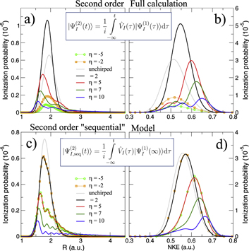
Figure 7. Ionization probability density as a function of the internuclear distance in (a) and (c) and as a function of the nuclear kinetic energy release in (b) and (d) for different values of the chirped parameter (see legend). (a) and (b) are the probabilities obtained by solving the full dimensional TDSE, while (c) and (d) correspond to the probabilities extracted using a 'sequential' model based on second order time-dependent perturbation theory as explained in the text.
Download figure:
Standard image High-resolution image4.1. Relationship between the chirp and an actual pump–probe time delay
We now analyze this effective pump–probe scheme in more detail. As mentioned in section 2.2, for Gaussian chirped pulses, equation (7), the double integral in equation (6) can be performed analytically even without the sequential approximation (taking here only the terms corresponding to absorption of photons), yielding

where  is the Faddeeva or complex error function, Δt = ωf − ωg − 2ω is the total detuning of the two-photon absorption process, and Δr = Δωfm − Δωmg = ωf − 2ωm + ωg is the frequency difference between the first and second transition. Due to the definition of chirped pulses that maintains the total pulse energy constant, the constant prefactor does not depend on the chirp parameter η (we have here neglected a constant η-dependent phase that could be removed by absorbing it in the definition of the pulse, equation (7)). Note that equation (13) only depends 'trivially' on Δt, specifically through a Gaussian function that ensures total energy conservation within the bandwidth of the pulse and induces a quadratic final-state-dependent phase. Importantly, the first line of equation (13) does not depend on m, the intermediate state index. All the wave-packet dynamics in the intermediate states, which is the relevant part for making a connection to pump–probe experiments, are thus encoded within the sum in the second line. Interestingly, this part of the expression does not depend on the laser frequency, but just on the involved transition frequencies, the pulse duration, and the chirp parameter. We also note that equation (13) is exact in the perturbative limit, and indeed reproduces the numerical results perfectly.
The sequential approximation in equation (12) is equivalent to approximating the Faddeeva function  in equation (13) as
  leading to

where we have defined  as the dipole transition element weighted by the pulse envelope for the relevant transition, and have omitted factors that do not involve m, i.e. that are constant for a given final state. Here, the relative phase of different intermediate state contributions depends linearly on η, but quadratically on the energy ωm (recall that Δr = ωf − 2ωm + ωg). This is in contrast to traditional pump–probe setups [52, 53], which feature analogous formulas in which the phase depends linearly on the intermediate state energy and time delay. As we have previously shown [27] and summarize here, the action of a chirped pulse can be mapped to a traditional pump–probe setup within this sequential approximation under the assumption that the dominant contributions are concentrated close to an average intermediate energy
  Expanding the exponent up to first order in δ, with
  then gives

where  is the effective time delay and the term quadratic in δ can be neglected for sufficiently small δ. For large enough values of η, the effective time delay τ matches the difference between the times when the instantaneous frequency
  is resonant with the average transition energies
  and
and  In summary, these expressions demonstrate that, within the validity of the sequential approximation, the chirped pulse acts like a conventional pump–probe setup, but with an effective time delay proportional to the average energy difference of the transitions of interest.
We next investigate whether this mapping still can be performed without the sequential approximation. The final-state amplitude can then be written as

The complementary error function  with complex argument does not correspond to a pure phase, and thus affects the relative amplitudes of the effective intermediate wavepacket. Indeed, it encodes the sign of the chirp by favoring contributions in which the second induced transition has higher (lower) energy than the first one, Δr > 0 (Δr < 0), for up-chirped (down-chirped) pulses, with other contributions suppressed more efficiently as
  increases. However, as can be seen in figure 8, both the absolute value and phase of
  are approximately constant when the chirp is chosen to correspond to the physically relevant transition, i.e. when Δr and η have the same sign (only positive values of η are shown since only the product Δrη enters the formula). For completeness, note that the divergence and rapid phase oscillation of F for large
  are canceled out by the exponential prefactor of the Faddeeva function in the full two-photon amplitude. In brief, this analytical approach demonstrates that the chirped pulse thus indeed provides a good approximation of a pump–probe setup, although with an additional modulation in the effective intermediate wave packet amplitudes compared to the sequential model or two-pulse pump–probe setups.

Figure 8. Absolute value (top) and phase (bottom) of the complementary error function contribution F to the two-photon amplitude.
Download figure:
Standard image High-resolution image5. Conclusions
Retrieving the dynamical processes occurring in atoms and molecules on the attosecond time scale is a challenging task that requires sources with attosecond stability, more than attosecond duration. We have shown a theoretical study using frequency-chirped ultrashort pulses to manipulate molecular ionization and to obtain a time-resolved image of the excited molecular dynamics. We have used  as testbed to perform ab initio simulations beyond the Born–Oppenheimer approximation and investigate two-photon molecular ionization with such chirped pulses. First, we have shown that for intermediate values of the chirp parameter and despite the decoherence introduced by the nuclear degrees of freedom, molecular ionization yields can be manipulated by tuning the chirp of a pulse, leading to a modulation of the ionization probability by up to one order of magnitude. Moreover, we have demonstrated that the interference patterns previously described in two-photon excitation of atoms using chirped pulses in the optical regime [49] remain observable in the context of UV/XUV photoionization. Nevertheless, because the final electronic states now belong to a continuum, an experimental observation of these interferences can only be achieved perfoming energy-differential measurements, for both atomic and molecular targets. The laser intensities and pulse durations employed are nowadays experimentally available [6, 54–56]. Moreover, the intensity of the signal retrieved is of the same order of that one found in a recent attosecond UV pump–UV probe experiment [57] where the ultrafast nuclear-electron dynamics in the excited hydrogen molecule is probed by monitoring the time-delay-dependent ionization probability. Therefore, the experimental feasibility of the proposed scheme mostly relies on the tunability of the spectral chirp [58–61].
We have further investigated how the chirp-dependent energy differential ionization yields actually reveal the wave packet structure and dynamics, triggered in the excited molecule, both in real and energy space, as proposed in [27]. Such dynamics can be retrieved by means of a sequential model, similar to those used to interprete experiments performed with standard pump–probe setup. In addition, we have presented an analytical solution for the full two-photon ionization problem that allows us to verify the validity this sequential picture, and formally demonstrates that single chirped pulses can indeed provide the same information as standard pump–probe setups.
Acknowledgments
This work was supported by the European Research Council (ERC) under grants no. 290853 XCHEM and ERC-2016-STG-714870 MMUSCLES and the Ministerio de Ciencia e Innovación (Spain) projects FIS2013-42002-R and FIS2016-77889-R. JF and AP acknowledge Ramón y Cajal contracts from the Ministerio de Economía y Competitividad (Spain). FM acknowledges support from the 'Severo Ochoa' (SEV-2016-0686), and FM and JF from the 'María de Maeztu' (MDM-2014-0377) Programmes for Centers of Excelence in R&D. Simulations have been performed in our XCHEM computer cluster hosted in the CCC facilities at UAM and thanks to the computer time allocated in Mare Nostrum BSC-RES.
: Appendix. Chirp-induced dynamics in the excited molecule
For completeness, we here discuss in detail the ultrafast dynamics triggered in the excited molecule for the whole range of chirp parameters investigated. Note that, because of the energetics of our molecular target and the chosen laser parameters, in the current work, we are mostly probing the dynamics associated to a vibronic wave packet in only the first excited state 2pσu. However, our scheme could easily be applied to other molecular targets where excitation to a higher excited state or a manifold of electronic states becomes relevant. As an example, we show the nuclear wave packet dynamics triggered by different up- and down-chirped pulses in the first excited electronic state, 2pσu (figure A1), and in the second excited state, 3pσu (figure A2). Since in  the population in the latter is three orders of magnitude smaller, its contribution to the ionization after absorption of the second photon is negligible. Similarly, for the down-chirped pulses, the wave packet dynamics seen in the first row in figure A1 is not retrievable in the ionization signal for the current laser parameters because the frequencies arriving later in time are too low to cause ionization. However, by properly tailoring the chirped pulse parameters, also these dynamics could be mapped into the final ionization channel.

Figure A1. Nuclear wave packets pumped into the 2pσu state for different chirped pulses (plotted in red lines). Upper panels: negatively chirped pulses. Bottom panels: positively chirped pulses with the same total pulse durations.
Download figure:
Standard image High-resolution image
Figure A2. Nuclear wave packets pumped into the 3pσu state for different chirped pulses (plotted in red lines). Upper panels: negatively chirped pulses. Bottom panels: positively chirped pulses.
Download figure:
Standard image High-resolution image