


Abstract
Eigen analysis has been a powerful tool to distinguish multiple processes into different simple principal modes in complex systems. For a non-equilibrium system, the principal modes corresponding to the non-equilibrium processes are usually evolving with time. Here, we apply the eigen analysis into the complex climate systems. In particular, based on the daily surface air temperature in the tropics (30° S–30° N, 0° E–360° E) between 1979-01-01 and 2016-12-31, we uncover that the strength of two dominated intra-annual principal modes represented by the eigenvalues significantly changes with the El Ni o/southern oscillation from year to year. Specifically, according to the 'regional correlation' introduced for the first intra-annual principal mode, we find that a sharp positive peak of the correlation between the El Ni
 o region and the northern (southern) hemisphere usually signals the beginning (end) of the El Ni
 o. We discuss the underlying physical mechanism and suppose that the evolution of the first intra-annual principal mode is related to the meridional circulations; the evolution of the second intra-annual principal mode responds positively to the Walker circulation. Our framework presented here not only facilitates the understanding of climate systems but also can potentially be used to study the dynamical evolution of other natural or engineering complex systems.
Export citation and abstract BibTeX RIS

Original content from this work may be used under the terms of the Creative Commons Attribution 4.0 licence. Any further distribution of this work must maintain attribution to the author(s) and the title of the work, journal citation and DOI.
1. Introduction
Complexities of climate systems are generally due to the existence of multi-scale phenomena with a wide variety of space and time scales [1]. Small-scale phenomena such as convection and precipitation [2] are driven by large-scale forces such as the extratropical cyclones, planetary-scale waves, and meridional circulations. The El Ni o/southern oscillation (ENSO) is one of the most important phenomena in this planet, referring to vary between anomalously warm (El Ni
 o) and cold (La Ni
 a) phases in the eastern Pacific, which can cause the global impacts on year-to-year time scales [3, 4].
In 1969, Bjerknes postulated that the Bjerknes feedback (the Walker circulation) was essential to the mechanism of the ENSO [5]. Still, the mechanism has not been fully understood [6]. The alternations between warm and cold phases are quite irregular in the El Ni o basin [7]. There is a controversy over whether the ENSO is controlled by stochastic processes [8]. Heat frequently exchanges between the ocean and atmosphere near the equator. Moreover, the energy is transported over a great distance from the equator to the polar regions by the general circulations [9, 10]. From the physics point of view, the ENSO could be triggered by small-scale and short-term processes, if the critical condition (long-range correlation or teleconnection) is satisfied in this system [11–13]. Although the ENSO has known as an inter-annual phenomenon, it was found to be coupling with intra-annual processes [14–17], even with the higher frequency processes [18, 19]. A significant intra-annual variation of the ENSO has been observed–El Ni
 o events tend to peak in boreal winter and fall rapidly in boreal spring [20, 21]. Some studies [22–24] showed that the ENSO combines with an annual cycle.
Eigen analysis has been a classic technique to distinguish multiple physical processes into a combination of some single processes and capture the individual feature. It is widely used in community detection, image recognition and empirical data analysis [25–27]. Also, it has emerged as a very popular tool in climate science called as the empirical orthogonal function (EOF) analysis [28] and been used to search for the features of the ENSO [29–31]. The inter-annual principal modes associated with the ENSO have been found based on the EOF analysis [22, 29]. Due to the multi-scale characteristics of climate in time and space, the interdisciplinary complex-based approaches such as complex networks [32–37] and wavelet analysis [38, 39] have been proved to be very powerful tools to study climate phenomena. Some recent studies have applied these complex-based methods to enhance the prediction skill of the El Ni o [40–42] and study its impacts [43, 44]. Actually, the essential of climate networks is the correlation matrix as well as the eigen analysis [45, 46]. Fast fluctuations of the correlations observed during El Ni
 o periods cause the links to break in the climate networks [47, 48].
Here, we use eigen analysis to study the intra-annual principal modes of daily surface air temperature (SAT). Previous studies mentioned above focused on the inter-annual principal modes for the deseasonalized data. However, the preprocess of removing seasonality could artificially change the annual cycles. Thus, we use the raw SAT data here in comparison to use the deseasonalized data. Furthermore, it is different with previous studies that we focus on the intra-annual principal modes for the correlation matrix in a 365 days' window and their temporal evolution with the time window. Previous EOF analyses assume that the eigenvalues and eigenvectors remain constant from year to year. Here, the intra-annual principal modes can change with time in the non-equilibrium system. These changes can be identified by fluctuations of the eigenvalues and eigenvectors. The eigenvalue plays an important role to describe the macroscopic properties of physical systems, which is related to the susceptibility of systems [49, 50]. The detailed spatial patterns are performed by the distributions of eigenvectors. This paper is organized as follows. Section 2 describes the materials and methods. In section 3 we present the results, and provide the conclusions in section 4.
2. Materials and methods
2.1. Data
The used raw data are daily SAT at 2 m and surface wind at 10 m provided by the European center for medium-range weather forecasts interim reanalysis (ERA-Interim) [51] on a 2.5° × 2.5° latitude–longitude grid over the tropics region (30° S–30° N,0° E–360° E), resulting in 25 × 144 = 3600 grids. The dataset spans the period between 1979-01-01 and 2016-12-31. El Ni o or La Ni
 a events are defined when the oceanic Ni
 o index (ONI) exceeds ±0.5 °C for a period of five months or more. The ONI is defined as the 3 month running mean of ERSST.v5 SST anomalies in the El Ni
 o 3.4 region (5° S–5° N, 190° E–240° E). To obtain the deseasonalized data, we subtract from each day's temperature the yearly mean temperature of that day. Specifically, if we take the raw daily SAT time series of a given grid to be Sy(t), where y is year and t is the day in a range from 1 to 365; the deseasonalized time series
  , where Ny is the total number of years from 1979 to 2016.
2.2. Methodology
2.2.1. Principal modes of temperature fluctuation
In a climate system consisting of N grids, the temperature of a grid i at time t within a time window of length d is defined as Si(t; T), where T represents the central time of the time window. The average temperature of grid i for the time window is calculated as

At the time t, the grid i has a temperature fluctuation  . The standard deviations of temperature for land and sea are very different. Thus we consider here the normalized fluctuation
 ![$\delta {\hat{S}}_{i}\left(t;T\right)=\delta {S}_{i}\left(t;T\right)/\sqrt{\left\langle {\left[\delta {S}_{i}\left(t;T\right)\right]}^{2}\right\rangle }$](https://content.cld.iop.org/journals/1367-2630/22/9/093077/revision2/njpabb89aieqn17.gif) . The correlation of temperature for the time window T between grids i and j is defined as
. The correlation of temperature for the time window T between grids i and j is defined as

which is the Pearson correlation coefficient. Using Cij(T) as its elements, we obtain then an N × N correlation matrix C(T) with N eigenvectors and eigenvalues. The eigenvector corresponding to eigenvalue λn(T) is bn(T) which satisfies the equation

The eigenvalues are numbered in the order λ1(T) ⩾ λ2(T), ..., ⩾ λN(T) ⩾ 0. The summation of all the eigenvalues satisfies ∑nλn = N.
The eigenvectors follow the condition

where δnl = 1 at n = l and δnl = 0 otherwise. All eigenvectors are normalized and orthogonal to each other.
Using the nth eigenvector bn(T), the nth principal mode can be obtained as

The correlation between principal modes an(T) and al(T) is

So different principal modes are independent for a certain T. The square amplitude of a principal mode is equal to the corresponding eigenvalue. Furthermore, we can shift the time T to obtain the evolution of eigenvalues and eigenvectors.
2.2.2. Regional correlation in principal modes
By equation (5),  can be considered as the summation of contributions from all principal modes

Combining equations (7) and (6) into (2), the correlation between girds i and j can be written as

To quantify the correlation of the nth principal mode between region A (such as the El Ni o 3.4 region) and region B (such as the northern or southern hemisphere), the 'regional correlation' is defined as

where NA and NB are total numbers of girds within region A and B respectively. To exclude noises of bin, we define Θin(T) = 1 for  and Θin(T) = 0 otherwise. The average value of bin is
  and we choose a threshold
  . The regional correlation
  reflects the relations between two specific regions, which is resulted by the nth principal mode. It also changes with the time T.
3. Results
We start to obtain the deseasonalized data as described in section 2.1. Since the seasonal cycle is 365 days, we take the length of time window d = 365. For a time window with its center in the month T, we can obtain the correlation matrix C(T) and do eigen-decomposition. With T shifted by one month each time, their evolution with the time window can be obtained for both the raw and deseasonalized data.
We calculate the intra-annual principal mode an(T) by equation (5). For example, figure 1(a), (c) show the principal modes a1(t; T) and a2(t; T) of the raw data with respect t at different T corresponding to a normal time (1994.01), an El Ni o time (1998.01), and a La Ni
 a time (2000.01) respectively. A dominant annual cycle in the first principal mode a1(t; T) is observed in figure 1(a). The mode a1(t; T) decreases as t from February to August, and increases from August to the next February. The second principal mode a2(t; T) is presented in figure 1(c), where an annual cycle is also observed. In comparison with figure 1(a), the annual cycle of a2(t; T) has a shift. It is reasonable that the annual cycle plays the dominant role in a1(t; T) for the raw data, since the influences of Sun are the deciding factors to result in the seasonal fluctuations of surface air temperature. For a2(t; T) of the raw data, figure 5(a) shows that the eastern Pacific is a prominent area whose seasonal cycle has been found to follow the southern hemisphere but it is shifted by a few months [52]. Thus, the annual cycle also domains in the second principal mode. Besides, we apply the spectrum analysis to the principal modes and find that the period 365 days is dominated for all the cases in figure 1 and their phases are similar for different years. The results indicate that the intra-annual principle modes of the deseasonalized data still exit a common annual cycle for different years (see figures 1(b) and (d)).
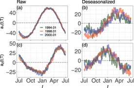
Figure 1. The first principal mode for (a) the raw data and (b) the deseasonalized data for different T: 1994.01, 1998.01 and 2000.01. (c), (d) Same as (a), (b) but for the second principal mode.
Download figure:
Standard image High-resolution imageTo further quantify differences of the intra-annual principal modes in different time T, we calculate the variances of the principle modes which are the eigenvalues (see equation (6)). The eigenvalues can represent the strength of principal modes. The fractions of the first eigenvalues and the second eigenvalues with T from 1979.06 to 2016.06 are shown in figures 2(a) and (c) for the raw data. The fraction λ1(T)/∑nλn(T) is more than 40%. The fraction of the second eigenvalue varies from 10% to 20%. For the deseasonalized data in figure 2(b) and (d), the fractions of the corresponding eigenvalues are smaller than those of the raw data, since temperature fluctuations are smaller in the deseasonalized data. The results show that the evolution of eigenvalues significantly changes with time for both the raw and deseasonalized data. For instance, the peaks of λ1(T)/∑nλn(T) for the raw data correspond to EI Ni o events and its valleys correspond to La Ni
 a events in figure 2(a). λ2(T)/∑nλn(T) in figure 2(c) is opposite to λ1(T)/∑nλn(T) in figure 2(a). For the deseasonalized data, it seems that both EI Ni
 o and La Ni
 a correspond to the peaks of eigenvalues in figures 2(b) and (d). Thus, the eigenvalues mainly describe the strength of intra-annual principal modes of temperature in response to the ENSO force.
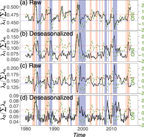
Figure 2. Fractions of the first eigenvalue λ1 as a function of time T (black solid line, left scale) for (a) the raw data and (b) the deseasonalized data. (c), (d) Same as (a), (b) but for the second eigenvalue λ2. Green dashed line is the ONI (right scale). Red and blue shades represent respectively El Ni o and La Ni
 a periods.
Download figure:
Standard image High-resolution imageWe show that the fractions of the first and second eigenvalues as a function of the ONI in figure 3. Figure 3(a) and (c) show that both the first and second eigenvalues for the raw data have a strong relevance to the ONI. The R coefficient between the fraction of λ1 and the ONI is characterized by their Pearson correlation coefficient, which is equal to 0.65 in figure 3(a). The R coefficient between the fraction of λ2 and the ONI is equal to −0.62 in figure 3(c). Moreover, the R coefficient between the fractions of λ1 and λ2 is equal to −0.75. This indicates that the first (second) principal mode is reinforced (weakened) during El Ni o periods. We also compare with the results of the deseasonalized data as shown in figure 3(b) and (d). Since their relations are nonlinear with the ONI, we use the absolute ONI here. The R coefficients for the deseasonalized data (see figure 3(b) and (d)) are positive and smaller than the absolute R coefficients of the raw data. The results indicate the better correlations for the raw data than the deseasonalized data. We also test other smaller eigenvalues such as the third and fourth eigenvalues. They do not show a significant correlation with the ONI or its absolute value.
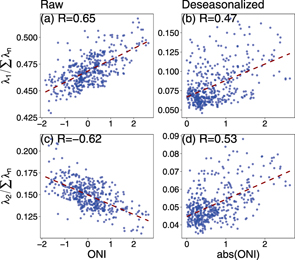
Figure 3. Fractions of (a) the first eigenvalue λ1 and (c) the second eigenvalue λ2 as a function of the ONI for the raw data. Fractions of (b) the first eigenvalue λ1 and (d) the second eigenvalue λ2 as a function of the absolute ONI for the deseasonalized data. Red dashed line is the regression line. The R coefficient is in top-left corner.
Download figure:
Standard image High-resolution imageTo understand spatial features of intra-annual principle modes, we study the spatial distribution of bn(T). An example is depicted in figure 4 for T from 1997.01 to 1998.10, which spans the strong 1997−98 El Ni o event. In the Jan of 1997, the ONI was −0.49 and increased to 0.74 in the May of 1997, which demonstrate the emergence of an El Ni
 o event. This event lasted until to the Aug of 1998. With the further decrease of the ONI, a La Ni
 a event appeared in the July of 1998 and lasted until 2001. The distributions of bi1 are divided mainly into two large clusters for the raw data in figure 4(a). One is in the northern hemisphere and has negative components. Another one is in the southern hemispheres and has positive components. In addition, there are two small clusters with negative components and located in the rainforests of Congo (Africa) and Amazon (South America). The components of the interface between two large clusters are nearly zero. The interface exists around the equator and varies greatly with time T.

Figure 4. Spatial distributions of components of the first eigenvector b1(T), where the time T is from 1997.01 to 1998.10 for (a) the raw data and (b) the deseasonalized data. They are the normal (1997.01–1997.04), El Ni o (1997.05–1998.05), and La Ni
 a (1998.07–1998.10).
Download figure:
Standard image High-resolution imageIn the normal phase at the beginning, the El Ni o 3.4 region (5° S–5° N, 190° E–240° E) belongs to the interface and the corresponding bi1(T) are nearly zero (see figure 4(a) for 1997.01). The temperature fluctuations in the region are nearly independent of the first principal mode. Later, the components bi1(T) in a part of the region become negative. The temperature fluctuations there are dominated by the first principal mode
  . The negative components (blue) in the El Ni
 o 3.4 region (see figure 4(a) for 1997.04 and 1997.07) result in the temperature fluctuations increases as a1(t; T) decreases from February to August (see figure 1(a)) in comparison with the normal phase. Then an El Ni
 o appeared, and the components in the El Ni
 o region gradually change from negative to positive. We can see that the components bi1(T) in a part of the El Ni
 o region become positive later (see figure 4(a) for 1998.04 and 1998.07). These positive components (red) can contribute the decrease of temperature and end the El Ni
 o to the La Ni
 a after next February. For the deseaonalized data in figure 4(b), the strong components mainly distribute in the eastern Pacific which are consistent with the distribution of temperature anomalies. Moreover, the components change with time T over the entire region.
The spatial distributions of b2(T) are shown in figure 5. For the second eigenvector of the raw data in figure 5(a), there are two large clusters with positive components in the Indian ocean and the eastern Pacific and their temperature fluctuations are coupled. At the beginning of 1997 (see figure 5(a) for 1997.01 and 1997.04), there is a large cluster with positive components in the eastern Pacific. With the emergence of El Ni o from 1997.07 to 1998.04 in figure 5(a), this cluster becomes smaller and weaker. Even a cluster with negative components appears in the region. After the end of El Ni
 o, there is a La Ni
 a and a cluster with positive components appears again in the eastern Pacific (see figure 5(a) for 1998.07 and 1998.10). For the deseaonalized data, the sizes of clusters in figure 5(b) are smaller than the clusters in figure 5(a). It is difficult to find a regular pattern for the deseaonalized data. Thus the spatial distributions of the eigenvectors for the raw data show a better relationship with the 1997–98 El Ni
 o event than the deseaonalized data as well as the eigenvalues.

Figure 5. Same as figure 4 but for the second eigenvector b2(T).
Download figure:
Standard image High-resolution imageTo analyze the relationship between the ENSO and the spatial distributions of bn for the raw data comprehensively, we calculate the regional correlation via equation (9) from 1979 to 2016. The regional correlation of the first principal mode for the raw data between the El Ni o 3.4 region and the northern region (5° N–30° N, 0° E–360° E) can be obtained as
  . Similarly we obtain the regional correlation
  between the El Ni
 o 3.4 region and the southern region (5° S–30° S, 0° E–360° E). The regional correlation
  (solid line) and
  (dashed line) are shown as functions of time T in figure 6(a). A large
  (
( ) represents that the El Ni
 o region is positively correlated with the north (south) region, as shown in figure 4(a). In normal phases, figure 6(a) shows that
  and
and  are close to zero. We find that
  has a peak before the emergence of (nearly 70%) El Ni
 o events in figure 6(a). This could imply a possible early warning signal for the El Ni
 o. Instead,
  has a sharp peak at the end of (nearly 90%) El Ni
 o events. Such correlation between the El Ni
 o region and the northern (southern) hemisphere for the first principal mode of the raw data could be driven by the Hadley circulation [53], which is a general meridional ocean-atmospheric circulation.
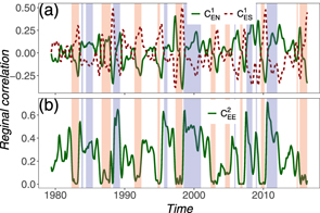
Figure 6. Regional correlation for (a) the first principal mode and (b) the second principal mode for the raw data. Red and blue shades represent respectively El Ni o and La Ni
 a periods.
Download figure:
Standard image High-resolution imageThe second principal mode of the raw data is dominated by the cluster components in the equatorial eastern Pacific (see figure 5(a)). Thus we calculate the regional correlation of the second principal mode for the El Ni o 3.4 region itself (like autocorrelation) as
  . Figure 6(b) shows that
  is strong during La Ni
 a phases and becomes weak during El Ni
 o phases. It indicates that the strength of the cluster in the El Ni
 o region is anti-correlated with the ONI in this region. The correlation coefficient between the ONI and
  is −0.76. The regional correlation
  is positively related to the Walker circulation, which is a zonal ocean-atmosphere circulation in the Pacific (the east–west surface temperature contrast reinforces an east–west air pressure difference across the Pacific basin, which in turn drives trade winds). During La Ni
 a, the Walker circulation becomes strong with the strong trade winds. During El Ni
 o instead, the Walker circulation becomes weak with the weak trade winds [2]. Moreover, the annual cycle of a2(t; T) in figure 1(c) is also associated with the seasonal variation of the Walker circulation which is very pronounced in January [54].
We further prove our conjectures by studying the daily surface wind field (10 m) which is used to character the zonal and meridional circulations. The wind is divided into meridional part V and zonal part U. For the northern region (0°–30° N, 190° E–240° E), the average magnitude  is calculated and presented in figure 7(a). We make the average for one year with its center in the month T. The average magnitude of V in the southern region (0°–30° S, 190° E–240° E) is denoted as
  . The results obtained are shown in figure 7(b). We can see that El Ni
 o events are accompanied usually by strong
  . In general,
  is larger than
  . This result further demonstrates that the connection between the equator and northern (southern) hemisphere becomes stronger during El Ni
 o in agreement with the results of the regional correlation
  and
and  in figure 6(a).

Figure 7. Mean V wind strength (a)  and (b)
  , and (c) mean U wind strength
  as a function of time T (black solid line, left scale). Green dashed line is the ONI (right scale). Red and blue shades represent respectively El Ni
 o and La Ni
 a periods.
Download figure:
Standard image High-resolution image
For the zonal part of wind, we calculate its average magnitude  in the Ni
 o 3.4 regions. The results obtained are depicted in figure 7(c). During El Ni
 o events, there are obvious decreases of
  as similar as
  in figure 6(b). We obtain that the correlation between
  and the mean V wind strength
  equals 0.35 (p-value <10−3); and the correlation between
  and the mean U wind strength
  is 0.47 (p-value <10−3). Both the correlation coefficients are significant. However, the wind strength
  does not always become weak during El Ni
 o events. It seems to show different behaviors for different El Ni
 o, i.e., the central Pacific El Ni
 o events such as 1994–93, 2004–05 and 2009–10 have the much stronger wind strength
  than the eastern Pacific El Ni
 o such as 1997–98 and 1982–83.
4. Conclusions
Here we studied the evolution of the principal modes in the climate system. Based on the daily SAT in the region (30° S–30° N, 0° E–360° E) for both the raw and deseasonalized data, we found that there exist two largest intra-annual principal modes corresponding to two annual cycles within one year. The temporal evolution of the intra-annual principal modes is investigated from 1979-01-01 to 2016-12-31 by sliding the one-year time window. We showed that the eigenvalues λ1 and λ2 significantly response to the ENSO variability for the raw data. The Pearson correlation coefficients between the fractions of the first and the second eigenvalues and the ONI are 0.65 and −0.62, which imply that the first (second) principal mode is reinforced during El Ni o (La Ni
 a) and weakened during La Ni
 a (El Ni
 o).
o).
The eigenvalues of the two intra-annual principal modes for the raw data have a stronger correlation with the ENSO than that for the deseaonalized data, as well as the spatial distributions of eigenvectors. We proposed a regional correlation to quantify the relations of temperature fluctuations between the El Ni o region and other regions for the raw data. In normal phases, the regional correlation for the first principal mode is very weak and the temperature fluctuations in the El Ni
 o region are dominated by the second principal mode. When the regional correlation of the northern hemisphere for the first principal mode becomes strong positive from February to August, the El Ni
 o event will occur with a high probability. With the evolution of the El Ni
 o event, the regional correlation of the southern hemisphere changes from negative to strong positive so that the temperature decreases fast after the next February. For the second principal mode, the autocorrelation of the El Ni
 o region has middle value during the normal phase and large value during the La Ni
 a phase, which correspond to normal and strong Walker circulation respectively. With the emergence of an El Ni
 o event, the autocorrelation becomes small in relation to a weak Walker circulation leading.
We suggest that the evolution mechanism for the ENSO is the competition between the first and second intra-annual principal modes for the raw SAT data, which are related to the meridional and zonal circulations respectively. This is demonstrated partly by the mean meridional and zonal surface wind field (10 m). The meridional circulations could drive the seasonal footprint from the northern and southern hemispheres to the El Ni o region such that the influences on the ENSO. Our method can also be used to study the dynamics of other non-equilibrium complex systems.
Acknowledgments
We are grateful to the financial support by the National Natural Science Foundation of China (Grant Nos. 61573173 and 72001213) and Key Research Program of Frontier Sciences, CAS (Grant No. QYZD-SSW-SYS019). Yongwen Zhang thanks the postdoctoral fellowship program funded by the Kunming University of Science and Technology. JF acknowledges the 'East Africa Peru India Climate Capacities—EPICC' project, which is part of the International Climate Initiative (IKI). The Federal Ministry for the Environment, Nature Conservation and Nuclear Safety (BMU) supports this initiative on the basis of a decision adopted by the German Bundestag. We also acknowledge the computational resources provided by HPC Cluster of ITP-CAS.