


Abstract
We investigate the four-wave mixing (FWM) nonlinearity in an ensemble of cold Rydberg atoms with each of them regarded as a double-ladder system. The interaction is studied from the view of generating a signal field in virtue of three applied lasers. Using an approach beyond mean-field theory, we solved the equations for the one-body and two-body correlators under perturbation, and show that the system possesses not only a local FWM nonlinearity, but also a much larger nonlocal nonlinearity due to the Rydberg–Rydberg interaction which can be further strengthened by increasing the atomic density. The results obtained may have promising applications in the quantum information processes involving the FWM nonlinearity, such as the generation of squeezed or entangled states.
Export citation and abstract BibTeX RIS

Original content from this work may be used under the terms of the Creative Commons Attribution 4.0 licence. Any further distribution of this work must maintain attribution to the author(s) and the title of the work, journal citation and DOI.
1. Introduction
Atoms excited to high-lying Rydberg states interact via strong and long-range dipole–dipole or van der Waals forces, and such strong interactions manifest as a well-known excitation blockade [1] in which an atom promoted to a Rydberg level shifts the energy levels of nearby atoms and suppresses their excitation. The blockade is of great interest for applications in quantum information [2] and provides the basis for numerous proposals, such as the photon–photon phase gates [3], atomic logical gates [4, 5], single-photon switch [6] and generating nonclassical state of light [7, 8].
Due to such pronounced nonlocal interaction between the atoms, the Rydberg atomic gases are regarded as a promising candidate for many-body correlated systems which act as effective tools to control the interactions between photons [9, 10]. One of such applications is to enhance nonlinearity [11–13] with the help of electromagnetically induced transparency (EIT). For example, the Kerr effect, as one of main topics in nonlinear optics with numerous applications in, such as single-photon switches and transistors [9], controlled quantum gates [14–16], quantum teleportation [17] and entanglement [18], can be greatly enhanced in Rydberg-EIT system [19–21]. Calculations beyond mean-field theory [21–25] attribute such improvement to the two-body or even three-body correlators based on perturbation method.
Motivated by the recent investigations on strengthening the Kerr nonlinearity, in this paper we study the enhancement of another third-order nonlinearity, namely, the four-wave mixing (FWM) process which has been used as an important resource for many quantum applications, such as quantum entanglement and steering [26–30], quantum cloning [31], generating correlated beams and photon pairs [32–35], constructing nonlinear interferometer [36] and quantum networks [37], as well as realizing optical nonreciprocity [38], etc.
The system that we are interested in is shown in figure 1(a) where three applied fields, specifically, a pumping field (Ωp), coupling field (Ωc) and a driving field (Ωd) illuminate the four-level atoms with a Rydberg state as the highest level to generate a signal (Ωs) with the efficiency determined by the third-order susceptibility. Investigations using the similar excitation schemes are reported, for example, to build a single-photon source by utilizing the Rydberg blockage of confined atoms in an excitation volume similar to, or smaller than that of the blockade sphere [39–41], or using the pumping and coupling fields to construct Rydberg dark-state polaritons for, e.g. the efficient light storage which can be retrieved by applying the driving field after a short time period [42, 43]. We also note the early experimental investigations on FWM in Rydberg gases of which the atomic density is too low to invoke significant Rydberg–Rydberg interaction [44–47]. In this paper, we study instead a (virtual) transition |1⟩ → |2⟩ → |4⟩ → |3⟩ → |1⟩ in an ensemble of cold Rydberg atoms of which the size is larger than the blockade sphere as schematically shown in figure 1(b), to show that the corresponding nonlinear susceptibility is significantly enhanced by the Rydberg–Rydberg interaction.
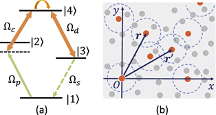
Figure 1. (a) The four-level atomic system with a Rydberg state |4⟩ illuminated by a pumping field Ωp, coupling field Ωc and a driving field Ωd, to generate signal field Ωs. (b) The coordinate system for calculating the Rydberg–Rydberg interaction, with the atom of interest located at origin. The blocked sphere caused by the interaction between Rydberg atoms (red dots) is schematically shown by the blue dashed circle. Inside each sphere, only one atom can be excited to the Rydberg state while excitations of other atoms (gray dots) are prevented. The correlation between the two Rydberg atoms (e.g. the one at position r and the one at origin) and three-atom correlation (including one more atom at r') are discussed in this paper.
Download figure:
Standard image High-resolution imageAt first glance, the nonlinear susceptibility of the FWM process has a small modulus, meaning that the generation of Ωs cannot be efficient, as the susceptibility is proportional to the product of the four relevant dipole-moment elements in which the ones associating with the transitions of Ωc and Ωd are much smaller than the other two. However, our calculations show that this is only true for the local interaction between the atoms and photons. When the Rydberg–Rydberg interation is considered, we need to evaluate the two-body correlator and take into account the contributions from all Rydberg atoms in the atomic gases. This leads to an increment in nonlinearity which is represented by a large nonlocal susceptibility.
The organization of this article is as follows: in section 2, we present the model and equations for the one-body and two-body correlators. Section 3 discusses the perturbation method we used to solve the equations. The properties of the local and nonlocal susceptibilities obtained from the solutions are analyzed as well. In appendix
2. Model and equations
Let us consider an ensemble of ultra-cold (for example, 87Rb) atoms each having a four-level double-ladder configuration as shown in figure 1(a) is loaded in a magneto-optical trap where the Doppler broadening caused by the thermal motion of atoms is significantly suppressed. Assuming that a strong coupling field (at angular frequency ωc, with Rabi frequency Ωc) drives the transition |2⟩ ↔ |4⟩ and a weak pumping field (ωp, Ωp) drives the transition between |1⟩ and |2⟩, then due to the presence of a strong driving field (ωd, Ωd), effective polarization could be built between the transition |1⟩ ↔ |3⟩, and subsequently resulting in the generation of a signal field (ωs, Ωs) by means of FWM process. The efficiency of the generation depends on the amplitude of (third-order) FWM nonlinear coefficient χ(3) which is the key subject that we are interested in this paper.
The excited state |4⟩ is a Rydberg state and assumed to be |60 S1/2⟩. The long-range interaction [48] between the Rydberg atom at position r and the one at position r' (see, figure 1(b)) is described by the potential V(Δr) = −C6/Δr6 with Δr = |r − r'|.
We assume that the electric fields can be written as  with c.c. standing for complex conjugate. Then the corresponding Rabi frequencies are
  , where μmn
with m, n = {1, 2, 3, 4} being the dipole moment of the transition |m⟩ ↔ |n⟩ that Ωi
drives. And the detunings are defined as Δp = ω21 − ωp, Δc = ω41 − ω21 − ωc, Δd = ω41 − ω31 − ωd. Δs = ω31 − ωs.
, where μmn
with m, n = {1, 2, 3, 4} being the dipole moment of the transition |m⟩ ↔ |n⟩ that Ωi
drives. And the detunings are defined as Δp = ω21 − ωp, Δc = ω41 − ω21 − ωc, Δd = ω41 − ω31 − ωd. Δs = ω31 − ωs.
Adopting the similar notations used in reference [24], we use  to denote the the transition operators for the atom at r, and it satisfies the commutation relation
 ![$[{\hat{S}}_{ab}(\mathbf{r},t),{\hat{S}}_{mn}({\mathbf{r}}^{\prime },t)]=[{\delta }_{an}{\hat{S}}_{mb}(\mathbf{r},t)-{\delta }_{mb}{\hat{S}}_{an}({\mathbf{r}}^{\prime },t)]{\delta }_{\mathbf{r}{\mathbf{r}}^{\prime }}$](https://content.cld.iop.org/journals/1367-2630/24/10/103002/revision2/njpac91e9ieqn4.gif) where δab
is Kronecker delta symbol. In the derivation to follow, we use
where δab
is Kronecker delta symbol. In the derivation to follow, we use  to represent the transition operator
  for the atom at origin, then under the electric-dipole and rotating-wave approximations, the Hamiltonian depicting the interaction between the atom (at origin) and the four fields takes the following form:
Here N0 is the atomic density and the symbol ∫d3
r stands for the integration  in spherical coordinates with Rb being the radius of the blockage sphere (see figure 1(b)). Then the features of the generation, absorption, as well as dispersion of the signal Ωs all hide in
  which is one of the one-body density-matrix elements governed by
 ![$\mathrm{i}\hslash \partial \langle {\hat{S}}_{mn}(t)\rangle /\partial t=\langle [{\hat{S}}_{mn}(t),\hat{H}]\rangle $](https://content.cld.iop.org/journals/1367-2630/24/10/103002/revision2/njpac91e9ieqn9.gif) . For instance, the equation of ρ31(t) reads
. For instance, the equation of ρ31(t) reads

it further relates to other elements, e.g. ρ41 whose time dependence is:
Here g31 = γ31 + iΔs and g41 = γ41 + i(Δc + iΔp). The whole (closed) set of the equations for the one-body density-matrix element is listed in the appendix  is one of the two-body correlators, generally defined as
  . Clearly, to solve the equations of the one-body density-matrix elements we need to find the values of the two-body correlators first. Akin to these one-body objects, the two-body elements satisfy a new set of the equations. For example, the equation for ρ44,41 is
It depends on other two-body correlators, we present in the following the equations for only two of them, so as to show the key features and save space in the meantime.

As we can see that the above equations contains three-body correlators, such as  . One can easily foresee that the motion of equations for the three-body correlators depend on the four-body ones and so on.
3. The local and nonlocal nonlinear susceptibilities
To achieve an effective FWM interaction, the excitation scheme illustrated in figure 1(a) uses a far-off-resonance pumping field Ωp to avoid the excitation of the atoms to level |2⟩. In virtual of the strong coupling field, a dark state [49] can be formed between |1⟩ and |4⟩ which further reduces the population on |2⟩. Further considering that the Rydberg–Rydberg interation causes energy shift which leads the blockade effect, then we can conclude that the population on |4⟩ is nearly negligible. Under the driving field Ωd, the FWM process, that is the virtual transition |1⟩ → |2⟩ → |4⟩ → |3⟩ → |1⟩ is initiated and results in the generation of Ωs without the other transition processes drawing energy from the inputs.
From this point of view, this double-ladder system is very similar to the double-Λ system that has been used in generating the entangled photon pairs [50, 51]. The difference is that the level |4⟩ is one of the ground levels in the double-Λ configuration, instead of a high excited Rydberg state. And we show in the following that this makes a big difference in the underlying physics.
The arrangement of the applied fields allows us to solve the equations of the density-matrix elements using the perturbation method with respect to the far-detuned pumping field and generated (weak) signal field. And the procedure is shown in figure 2 with panel (a) representing our original system. First, we expand the one-body elements with respect to Ωs as


Figure 2. Hierarchy of perturbation. The original system (a) is expanded with respect to the signal field (column b). We only consider the (0)-order system in panel (b1) here. The (1)-order system in panel (b2), and the following other-order systems related to Raman enhancement, Kerr nonlinearity and more higher-order effects experienced by the signal are out of the scope of this article. The (0)-order system is further expanded with respect to the pumping field (column c). As we can see that the order of perturbation is represented by the number of arrows of Ωp. The two-body correlator that interests us  seats on the
  order. And the corresponding panel follows next to (c3), however, is not explicitly shown.
Download figure:
Standard image High-resolution imageAnd the (0)-order equations obtained from the perturbation is simply the equations (A1)–(A7) listed in appendix  is built between |1⟩ and |3⟩, and illustrated vividly in panel (b1) that |1⟩ is connected with |3⟩ by the three applied fields. Naturally, the polarization takes a form of
  and leads to the generation of the signal depicted by the effective Hamiltonian [52, 53] that
  with
with  associated with the creation operator at ωs. We shall not further discuss in detail about the generation but only focus on coefficient χ(3). And the first-order system shown in (b2) is not discussed either in this paper, as it relates to the absorption and dispersion of the signal field after being generated, or of a field that is deliberately applied. The solution of
  provides the exact result of the nonlinear coefficient. However the result is still quite complex. Fortunately, the ladder-type EIT system (|1⟩ − |2⟩ − |4⟩) employs a far-detuned pumping field which naturally becomes our next perturbation parameter with its zeroth-order system shown in panel (c1), the first-order system in panel (c2) and the second in (c3). The corresponding expansion of the elements is

Note that the order of perturbation over Ωp is emphasized by angle brackets  in the superscripts. The
  -order system in panel (c1) is described by a set of equations with Ωp = 0 and Ωs = 0. Then one can easily see that this is a trivial system. Without the pumping and the signal, the atoms stay on the ground state and the corresponding elements of density matrix are zeros except
  . Then the
  -order system in panel (c2) with the corresponding equations listed in appendix
Here α = g31(|Ωc|2 + g21
g41) + g21|Ωd|2. The polarization built between |3⟩ and |1⟩ is formed via two different mechanisms represented by the two terms on the right-hand side of equation (5). An atom acting with the applied field as a independent (isolated) object leads to the generation of Ωs via a local nonlinearity. Considering the definitions of the Rabi frequencies and the polarization  , we find the corresponding coefficient is

With

And N0
U0 has a dimension of a third-order nonlinear susceptibility. In other words, if the level |4⟩ is not a Rydberg state, then the atomic gases would provide a nonlinearity whose strength is well modeled by  . However the level |4⟩ being a Rydberg state with a extreme long lifetime makes the local FWM process less efficient because μ42 and μ43 are much smaller than that of a transition involving only the non-Rydberg states.
The second term in equation (5) comes from the RydbergRydberg interaction and we show in the following that this part of interaction dominants in the FWM process. Note that ρ44,41(r, t) in equation (5) is a full-order quantity with respect to Ωp. We follow a similar procedure as in equation (4) to expand the two-body correlators as


The  -order elements
  are zeros since the probability of finding an atom on Rydberg state is zero without pumping and signal [see, panel (c1)]. The
  -order elements
  are zeros as well, due to the fact that the probability of finding a Rydberg atom located at r is still very small under the large-detuned pumping (at most on the second order of Ωp) [24].
Calculations on perturbation show that the  -order non-trivial elements (corresponding to panel (c3)) belongs to two sets of closed equations which are presented in matrix forms as equations (A10) and (A11) in appendix
  , and based on equation (3a), we have

The above equation depends on other  -order two-body elements, such as
  and
and  . Based on equations (3b) and (3c), they satisfy


The whole set of the algebraic equations for the  -order two-body elements has 27 unknowns including
  ,
,  and
and  which are listed in appendix
  -order equations relate to the
  -order one/two-body elements. And the
  -order elements depend on
  -order elements whose equations can be easily solved. Unfortunately, the solution to
  does not have a compact form, but we managed to write the expression into a power series with respect to Ωc and Ωd:

With
With m = 2, 3, ..., and n = 1, 2, .... The parameter α is defined in the previous discussion and β(r) = g41 + Γ42 + Γ43 + iV(r). Q(m, n) represents a general coefficient of the series. The exact solution of  should include all terms of the above expansion, and we have to calculate it numerically. From the equation (11) we can see that the resultant nonlinear coefficient depends on the squared modular of the coupling and driving Rabi frequencies, suggesting that nonlocal FWM process is dressed by the strong fields.
Substituting equations (10) and (11) into equation (5), we find nonlocal nonlinear coefficient is

In evaluating (12), we first determine the value of Rb, which under large pumping detuning, is ![${R}_{\mathrm{b}}=\sqrt[6]{{C}_{6}/{\delta }_{\text{EIT}}}$](https://content.cld.iop.org/journals/1367-2630/24/10/103002/revision2/njpac91e9ieqn45.gif) with
with  [13, 54], then the result is obtained from the integral with simple calculations, and is shown in figure (3).
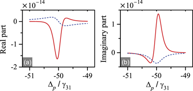
Figure 3. The local (blue dashed line) and nonlocal (red solid line) FWM susceptibilities under different pumping detuning Δp/Γ31. Γ42 = Γ43 = 2π × 3 kHz, Γ21 = Γ31 = 2π × 6 MHz, μ42 = μ43 = 0.01ea0, and μ21 = μ31 = 4.23ea0, C6 = −2π × 140 GHz μm6. Δc = 50γ31, Δd = −50γ31. Ωc = Ωd = 20γ31, and Ωp = 0.1γ31. The atomic density N0 = 9.0 × 1010 cm−3.
Download figure:
Standard image High-resolution imageBased on the results of Re  in figure 3(a) and Im
  in (b), we see that the nonlocal nonlinearity reaches its maximal strength at the double-photon resonance Δc + Δp = 0. This is physically intuitive as, under the same condition, the maximal coherence between |1⟩ and |4⟩ is achived. The center frequency of the generated field must satisfy Δp + Δc = Δd + Δs due to the conservation law of the energy. And for the parameters we used in figure 3, Δs = 50γ31.
As comparison we plot the local nonlinear susceptibilities in figure 3 as well to show that amplitude of  is much larger than that of
  at the given atomic density. The local nonlinearity comes solely from the interation between the photon and the atoms which can be viewed, as we stated before, a coherence between |1⟩ and |3⟩ built by the three applied fields leading to a polarization that induces the emission of the signal.
On the other hand, the nonlocal nonlinearity has a different mechanism. In virtue of the coupling and pumping field, a few atoms are excited to the Rydberg states and repel each other via the extra large dipole moments. This causes the addition potential energy V(r) which at the same time suggesting the existence of a tendency that the atomic gases would reduce its energy to a low state. Such tendency corresponds to the two-body element in equation (5), that is  , a correlation between probability of the atom at r staying on Rydberg state |4⟩ and that of anther Rydberg atom (at origin) jumping to the ground state. Since the two operators commutate with each other, the same argument can be made when interchanging the two atoms. Of course, such transition from |4⟩ to |1⟩ is unpractical due to the same parity of two levels. However with the help of driven field (
 in equation (5)), it manifest as a dominant part of the effective polarization and strengthen the FWM process.
Clearly, higher atomic density leads to shorter distance between atoms, thus significantly increases the two-body correlation and results in a much larger nonlinearity. In figure 4 we show the real part (a) and the imaginary part (b) of  as a function of atomic density. Comparing with the local part of nonlinear coefficient,
  is increased more significantly with the atomic density. Note that the method we used here requires a limitation on the atomic population so that we only need to consider the two-body elements without taking into account of the correlation between three or even more atoms. We can roughly estimate the proper atomic density via relation
  which means that given a blockage sphere and its close-packed one, in the space they occupy which is approximately a sphere having a radius of 3Rb, two atoms can be excited to Rydberg states with considerable opportunity, but never for three. For our parameters that leads to a condition that the proper atomic density should be smaller than 1.0 × 1011 cm−3.

Figure 4. The atom-light part (blue dashed line) and the Rydberg–Rydberg part (red solid line) of the nonlinear coefficient under different atomic density N0. Δc = 50Γ31, Δd = −50Γ31, and Δp = −50Γ31. Other parameters are the same as in figure 3.
Download figure:
Standard image High-resolution image
The possible experimental setup would be very similar to the system used in reference [44]. And since  is proportional to N0, while
  is proportional to
  , see equations (6) and (12). One can verify the mechanism of the generation of Ωs by examining the relation between the count rate of Ωs (proportional to squared modulus of the nonlinear susceptibility [50, 55]) and the atomic density. The nonlinearity based on Rydberg–Rydberg interaction would manifest itself as a dependence of the count rate on
  .
.
4. Conclusions
The FWM nonlinearity plays important roles in lots of applications in quantum information. And in this paper, we have investigated the enhancement of the third-order FWM nonlinearity via the correlation between two Rydberg atoms. Using the one-body and two-body elements of the density matrix, we solved the associated equations using perturbation method and show that the polarization which is induced by the pumping, coupling and driving field, and responsible for generating the signal field is composed of a local part from the interaction between atoms and photons and a nonlocal part due to the Rydberg–Rydberg interaction. Using a Rydberg state with n = 60 as an example, we show via the numerical results that the nonlocal nonlinear susceptibility dominates in the total nonlinear coefficient. For the Rydberg state with a even larger quantum number, beside the above mentioned result, one finds that the Rydberg–Rydberg interaction becomes stronger and that leads to a larger blockade sphere. If we only focus on the two-body correlation, then a relatively low atomic density should be adopt and calculations show that the nonlinearity is actually weaker owning to the relation  . With a higher atomic density, the three-body correlation should be considered and the nonlinearity could be further enhanced.
Acknowledgments
The work is supported by the National Natural Science Foundation of China (No. 12074061), the Fundamental Research Funds for the Central Universities (No. 2412020FZ028) and the Scientific and Technological Research Program of Jilin Education Department (No. JJKH20211280KJ).
Data availability statement
No new data were created or analysed in this study.
Appendix A.: The equations for the one-body and two-body density-matrix elements
For simplicity, we use complex decay rates gmn in the following equations, and they are defined as the composed of decoherence rates and detunings. g21 = γ21 + iΔp, g31 = γ31 + iΔs, g41 = γ41 + i(Δc + iΔp), g32 = γ32 + i(Δs − iΔp), g42 = γ42 + iΔc, g43 = γ43 + iΔd. The equations for one-body equations for


Equations for ρ31, ρ32 and ρ41 are presented in the main text as equations (2a) and (2b), respectively. In the above equations, the phase-matching condition Δs = Δc + Δp − Δd is already assumed. Under the double perturbation we find that the  -order equations for one-body elements are

Here  . In order to solve the
  -order equations for the two-body elements we also need the value of
  -order one-body element, and they reads
The nonzero two-body elements on  order are the solutions to two set of closed equations. In matrix form, they are
With M1 = −g12 − g21, M2 = −g12 − g31, M3 = −g12 − g41, M4 = −g13 − g21, M5 = −g13 − g31, M6 = −g13 − g41, M7 = −g14 − g21, M8 = −g14 − g31, M9 = −g14 − g41. M10 = −2g21, M11 = −g21 − g31, M12 = −g21 − g41, M13 = −2g31, M14 = −g31 − g41, M15 = −2g41 − iV.
The  -order equations depends on the above
  -order elements. To obtain
  we need to solution a set of equations with 27 unknowns, and they are:
They are obtained following the same procedure of finding the matrices of  -order equations. The matrix equation are not shown here since the size of the matrix is too large.