

Abstract
We review the use of young low mass stars and protostars, or young stellar objects (YSOs), as tracers of star formation. Observations of molecular clouds at visible, infrared, radio and X-ray wavelengths can identify and characterize the YSOs populating these clouds, with the ability to detect deeply embedded objects at all evolutionary stages. Surveys with the Spitzer, Herschel, XMM-Newton and Chandra space telescopes have measured the spatial distribution of YSOs within a number of nearby (<2.5 kpc) molecular clouds, showing surface densities varying by more than three orders of magnitude. These surveys have been used to measure the spatially varying star formation rates and efficiencies within clouds, and when combined with maps of the molecular gas, have led to the discovery of star-forming relations within clouds. YSO surveys can also characterize the structures, ages, and star formation histories of embedded clusters, and they illuminate the relationship of the clusters to the networks of filaments, hubs and ridges in the molecular clouds from which they form. Measurements of the proper motions and radial velocities of YSOs trace the evolving kinematics of clusters from the deeply embedded phases through gas dispersal, providing insights into the factors that shape the formation of bound clusters. On 100 pc scales that encompass entire star-forming complexes, Gaia is mapping the young associations of stars that have dispersed their natal gas and exist alongside molecular clouds. These surveys reveal the complex structures and motions in associations, and show evidence for supernova driven expansions. Remnants of these associations have now been identified by Gaia, showing that traces of star-forming structures can persist for a few hundred million years.
Export citation and abstract BibTeX RIS
1. Introduction
Over the past thirty years, there has been a rapid advance in our understanding of the evolution of baryonic matter from the Big Bang to galaxies containing richly structured interstellar mediums. One of the chief products of this evolution are low mass (≤1 M⊙) stars, which are the dominant form of stellar mass produced in the baryonic cycles of galaxies. The dominance of low mass stars is a consequence of their lifetimes and their status as the primary product of star formation. The initial mass function of star-forming regions and clusters peaks around 0.25 M⊙ and decreases with a Salpeter power-law form for masses in excess of 1 M⊙ (Salpeter 1955; Bastian et al. 2010). Approximately 40% of the initial stellar mass and 80% of all stars formed have masses between 0.08 and 1 M⊙.
The goal of this review is to better establish low mass stars as tracers of the star formation process over the spatial scales of clusters, associations and molecular cloud complexes. It builds on an unparalleled, two decade era of multi-wavelength surveys with space-based telescopes as well as ground-based and airborne observations. These near-field star formation studies are producing a deeper understanding of star and cluster formation in local regions of our galaxy and setting the stage for future studies probing more distant and diverse environments in our galaxy and others.
Molecular clouds were first efficiently surveyed for embedded low mass stars with near-IR detector arrays in the 1990s (e.g., Lada 1992; Zinnecker et al. 1993). Surveys with the Spitzer Space Telescope, Herschel Space Observatory, XMM-Newton, and Chandra Space Telescope have since provided the means to identify and characterize low mass young stellar objects (hereafter: YSOs) in young clusters and molecular clouds (e.g., Allen et al. 2007; Evans et al. 2009; Stutz et al. 2013; Kuhn et al. 2015b). Gaia has measured the parallaxes and proper motions of the less embedded stars in clusters and molecular clouds, as well as the more evolved associations of young stars outside the clouds (e.g., Kounkel et al. 2018; Kuhn et al. 2019).
Despite their numbers, the faintness of young low mass stars limits our ability to efficiently identify and study them beyond 2.5 kpc. Existing surveys of the molecular clouds, associations and clusters within 500 pc of the Sun have produced the most complete censuses of YSOs. These are complemented by surveys of clouds and clusters between 500 pc and 1 kpc which include more high mass star-forming regions; these are needed to study how environment and feedback from massive stars shapes star and cluster formation. Observations of regions between 1 and 2.5 kpc include complexes comparable to those studied in other galaxies. The Cygnus-X region in particular provides a relatively nearby (1.4 kpc) example of the massive star-forming complexes found in other galaxies (Beerer et al. 2010; Rygl et al. 2012; Kryukova et al. 2014; Pokhrel et al. 2020). Surveys of the nearest clouds, however, are essential for understanding biases in studies of >500 pc regions.
The James Webb Space Telescope (JWST) and forthcoming extremely large telescopes will extend surveys for young low to intermediate mass stars to more distant regions of our galaxy as well as nearby galaxies such as the LMC. Studies of more distant galaxies will continue to depend on high mass stars, partially resolved massive star clusters, and the integrated light of older low mass stars as tracers of star formation (e.g., Bastian et al. 2010; Krumholz et al. 2019). Although observations beyond the nearest 2.5 kpc are needed for a representative view of star formation in the universe, their interpretation requires insights from local studies.
2. Questions and Scope
We will overview how surveys of low mass YSOs are addressing the following questions about the star formation process:
- 1.What are the rates, densities and efficiencies of star formation in molecular clouds, and how do they vary with environment?
- 2.What are the differences between diffuse and clustered star formation, and how do they depend on cloud properties?
- 3.What is the duration of cluster formation, and during this time, what processes shape the structure and kinematics of clusters?
- 4.How does star formation in cloud complexes produce a mixture of bound clusters and unbound associations, and how long do these assemblages persist in the galactic disk after star formation ends?
This review focuses on observational studies, and we include theoretical approaches only where they directly pertain to the interpretation of observational results or provide necessary context for the observations. Reviews of theory can be found in Krumholz et al. (2014, 2019), Longmore et al. (2014), Krause et al. (2020), Ballesteros-Paredes et al. (2020). A rigorous dialog between observations and theory is beyond the scope of this review. Instead, our goal is to build a foundation for such a dialog.
We will concentrate on nearby (<1 kpc) clouds and complexes with particular emphasis given to the Orion region. Although this sample is not representative of the diverse star-forming environments found in our galaxy and others, it can provide a detailed understanding of star formation over a considerable range of environmental conditions. Studies of these nearby regions include extensive observations of specific examples that complement results drawn from large samples, and this review will contain insights drawn from both samples and examples.
Ultimately, insights from these near-field studies will need to be extrapolated to the full range of gas densities, radiation fields, metallicities and tidal fields present in galaxies. This will require a detailed physical understanding of nearby regions and input from the rich samples of more distant clusters and clouds inhabiting diverse environments in our galaxy and others.
We will not discuss the IMF, although fundamental questions remain. Does the IMF vary, and if so, what environmental factors control its form? Is there primordial mass segregation within clouds and clusters? For a discussion of how surveys of low mass stars are helping resolve these questions, we refer the reader to Bastian et al. (2010), Kirk & Myers (2011, 2012), Hsu et al. (2013), and Luhman (2018).
In Section 3, we overview current observational methods for identifying and characterizing YSOs. Section 4 introduces methods for measuring the spatial distribution of YSOs and discusses analyses of YSO surface densities in star-forming regions. The determination of star formation rates, efficiencies, and relations in molecular clouds is the topic of Section 5. In Section 6, the demographics, properties and evolution of clusters are discussed. Finally, the evolution of clusters and association brings us from cloud to galactic scales in Section 7. The results are summarized in Section 8 and the appendices elaborate on several analyses described in the text.
3. Techniques for YSO Identification
Tracing star formation with low mass YSOs requires the capability to efficiently detect and identify young stars and protostars over large swaths of the sky. Space-based infrared and X-ray observatories, such as Chandra, XMM-Newton, Spitzer, WISE and Herschel, have identified and characterized low mass YSOs across fields many square degrees in extent with modest levels of contamination. The censuses obtained with these telescopes have been augmented with ground-based visible, near-IR and radio data and airborne IR data. More recently, astrometry with Gaia is providing a new means for identifying members through parallaxes or proper motions, although the wavelengths used by Gaia are not well suited for detecting embedded stars. In this section, we discuss the identification and classification of YSOs, emphasizing the strengths and weaknesses of each technique.
3.1. Mid-IR Imaging
The sensitivity of Spitzer at wavelengths longward of 3 μm fueled a revolutionary advance in mapping the distribution of YSOs with dusty disks and infalling envelopes (e.g., Allen et al. 2004, 2007; Gutermuth et al. 2004; Megeath et al. 2004; Muzerolle et al. 2004; Whitney et al. 2004; Harvey et al. 2007). At these wavelengths, the emission from circumstellar dust outshines the stellar photospheres and is easily detected by Spitzer. Dusty YSOs can be identified and classified though a variety of methods: fitting model spectral energy distributions (SEDs) to the photometry (Robitaille et al. 2007; Povich et al. 2013), using multiple color and magnitude criteria (Rebull et al. 2007; Gutermuth et al. 2009; Kryukova et al. 2014; Megeath et al. 2016), or a combination of those methods (Harvey et al. 2006, 2008). Figure 1 compares the application of different approaches on the LkHα101 cluster.
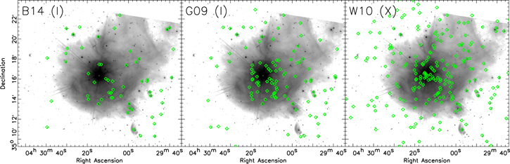
Figure 1. A comparison of different methods for identifying YSOs. These data show the YSOs (diamonds) identified toward the LkHα101 young cluster using Spitzer+2MASS data (B14, Broekhoven-Fiene et al. 2014), Spitzer+2MASS data with alternative identification criteria (G09, Gutermuth et al. 2009), and a combination of Spitzer, 2MASS and Chandra data (W10, Wolk et al. 2010). The 8 μm image in the background shows the bright IR nebulosity toward this region. While the Spitzer data is only identifying dusty YSOs, the Chandra data also finds young stars without disks or with optically thin disks.
Download figure:
Standard image High-resolution imageSpitzer and 2MASS provide photometry in ten wavelength bands from 1.2 to 160 μm. Surveys for dusty YSOs rely primarily on the 1.2–24 μm data due to the low angular resolution of the Spitzer 70 and 160 μm imaging. To maximize the completeness of the sample of YSOs, these methods typically do not require detections in all eight bands, and multiple criteria utilizing different combinations of the bands are often used to identify young stars (Gutermuth et al. 2009; Megeath et al. 2012). In regions with bright nebulosity, criteria using a combination of ground-based H and K-band and Spitzer 3.6 and 4.5 μm band photometry enhance completeness. In these bands, the contrast between YSOs and nebulosity is the highest. Other criteria are required to detect sources that are deeply embedded or whose disks are primarily detected at wavelengths >4.5 μm (e.g., Winston et al. 2007; Gutermuth et al. 2008). While the 2MASS point source catalog provides all-sky coverage in the J, H and Ks-bands, deeper NIR data bring higher sensitivities and angular resolution that can enhance completeness (e.g., Gutermuth et al. 2004; Allen et al. 2008; Masiunas et al. 2012; Povich et al. 2013; Willis et al. 2015; Großschedl et al. 2019).
There are limitations to these approaches. Reddening in the Spitzer bands, as given by the molecular cloud extinction laws of Flaherty et al. (2007) and Chapman et al. (2009), can affect the classification of YSOs. Highly reddened pre-main sequence (pre-ms) stars with disks can be misclassified as protostars (Kryukova et al. 2012; Dunham et al. 2015). Some YSO classification schemes are constructed around reducing such biases in YSO characterization (e.g., Gutermuth et al. 2008, 2009). Another limitation is that young stars without optically thick disks or infalling envelopes cannot be reliably identified, particularly if the stars are not detected in the Spitzer 24 μm band. This includes stars with no disks, optically thin disks, or disks with large inner holes (Winston et al. 2010; Cieza et al. 2012, 2013; Dunham et al. 2015).
Photometry covering the 3.6–24 μm range can also be used to estimate the luminosities of protostars. Determining the SED slopes and integrated fluxes of protostars over this wavelength range, Kryukova et al. (2012) and Dunham et al. (2013) found empirical relationships between the slopes and fluxes and the bolometric luminosities of protostars. The relationships can be used when far-IR data is not available.
The primary sources of contamination are galaxies, particularly active galactic nucleus (AGN), that are not spatially resolved by Spitzer. To minimize their numbers, color and magnitude criteria are applied to remove likely contaminants (Gutermuth et al. 2009; Kryukova et al. 2014) or to assign a probability that a source is a background galaxy (Harvey et al. 2007). These methods utilize data from wide-field extragalactic surveys to define the colors, magnitudes and densities of galaxies (Harvey et al. 2007; Gutermuth et al. 2009). Nearby reference fields are also used to estimate the level of contamination (Megeath et al. 2012). For regions observed against the galactic plane, contamination by AGB stars must also be considered (Robitaille et al. 2008). Most recently, Chiu et al. (2021) and Kuhn et al. (2021) applied machine and statistical learning techniques to separate YSOs from contamination, using YSO catalogs from nearby clouds as training sets.
WISE brought the ability to identify dusty YSOs over the entire sky, although with lower sensitivities and angular resolutions. Given the bright nebulosity in the mid-IR, the WISE data is susceptible to source confusion, particularly in the 22 μm wavelength band (e.g., Gutermuth & Heyer 2015). Different schemes have been suggested for identifying sources including SED slopes (Großschedl et al. 2019) and color criteria (Koenig & Leisawitz 2014; Fischer et al. 2016). The adopted criteria can be adjusted and optimized for the level of background contamination and source confusion (e.g., Pillitteri et al. 2017). Toward the L1641 region of the Orion A cloud, which lacks bright nebulosity, Großschedl et al. (2019) recovered 59% of the Spitzer identified dusty YSOs with the WISE data. Recently, Marton et al. (2019) combined WISE and Gaia data to find YSOs using machine learning.
Spitzer surveys of nearby star-forming regions also suffer from a spatially varying incompleteness, particularly in areas containing bright nebulosity (Gutermuth et al. 2009). Megeath et al. (2016) found that the sensitivity to point sources decreased as the median absolute deviation (MAD) of the signal in a field increased. The increase in the MAD is typically due to the presence of highly structured mid-IR nebulosity, which is commonly found in star-forming regions, although other stars can contribute to the MAD in crowded fields. They estimated that the fraction of detected stars dropped to about 10% in the brightest parts of the Orion Nebula compared to regions with only faint nebulosity (Figure 2). Since the brightest nebulosity is found in the rich clusters that typically contain OB stars, the detection rate of YSOs is systematically lower in fields with high YSO densities. This bias can be corrected by using X-ray data or by using the detection rates of fake stars in the mid-IR images, as described by Megeath et al. (2016, also see Figure 2).

Figure 2. A demonstration of how X-ray identified YSOs can be used to correct for biases in Spitzer surveys toward bright nebulae (Megeath et al. 2016). Left: comparison of Chandra and Spitzer identified YSOs in the center of the Orion Nebula Cluster. The background figure is the Spitzer/IRAC 3.6, 4.5 and 8 μm image of the nebula. This region is characterized by bright, spatially varying nebulosity which limits the detection of the mid-IR sources. The green dots are the IR-excess sources identified by Spitzer, the blue dots are X-ray sources with near-IR analogs found by the COUP survey and not identified by Spitzer. These include both diskless young stars and stars where confusion with the bright mid-IR nebulosity precludes their detections. Right: the surface density of YSOs vs. radius from the center of the nebula. The red curve is for YSOs identified by Spitzer while the green curve is that augmented by the COUP data.
Download figure:
Standard image High-resolution image3.2. X-Ray Imaging
X-ray surveys with the Chandra Space Telescope and XMM-Newton are also producing censuses of YSOs in clusters as well as entire molecular clouds (e.g., Pillitteri et al. 2013; Kuhn et al. 2015b), while the ongoing X-ray eROSITA survey will obtain a homogeneous selection of young stars across much of the sky. These observatories primarily detect X-rays from magnetically driven activity in the coronae of young stars (e.g., Feigelson & Montmerle 1999). The deepest X-ray survey of a star-forming region to date is that of the Chandra Orion Ultradeep Project (COUP), which obtained a 9.7 days exposure of the central region of the ONC (Feigelson et al. 2005). These data detect X-ray emission from 90% of the member stars. These stars have X-ray to bolometric luminosity ratios 1000 times that of the Sun and show fractional X-ray luminosities as large as  (Preibisch et al. 2005). The emission is highly variable, and flares can increase the X-ray flux by as much as a factor of 100 for tens of hours (Wolk et al. 2005).
X-rays in the energy regime probed by Chandra and XMM-Newton (0.5–8 keV) are relatively unaffected by interstellar absorption and can be used to detect embedded populations. In addition, X-ray emission is a signature of young stars that does not require the presence of disks or envelopes, and therefore can identify diskless stars. X-ray surveys are also not affected by the bright nebulosity found in the mid to far-IR. Although a complementary near-IR detection is usually required to confirm an X-ray source as a YSO (Getman et al. 2005), the comparatively faint nebulosity at near-IR wavelengths results in surveys which are less biased by nebulosity than mid-IR surveys (Figure 2).
The disadvantage of X-ray observations is incompleteness. Although COUP detected almost 90% of the YSOs in the Orion Nebula (Megeath et al. 2016), surveys of 200–500 pc regions with more typical integration times of many tens of kiloseconds often detect 30%–50% of the Spitzer-identified YSOs (e.g., Winston et al. 2010; Pillitteri et al. 2013). The undetected sources are less active or lower mass stars that are fainter at X-ray wavelengths and may only be detected during flares (Preibisch et al. 2005). For this reason, X-ray surveys, particularly with Chandra, have focused primarily on clusters (e.g., Winston et al. 2011; Kuhn et al. 2014). In comparison, cloud surveys, such as the XMM-Newton survey of Orion A, lack the sensitivity of cluster observations (Pillitteri et al. 2013).
The X-ray flux is dependent on the bolometric luminosities or surface areas of stars, although with an order of magnitude of scatter (Preibisch et al. 2005; Winston et al. 2010). This scatter, and the rapid evolving luminosities of pre-ms stars, makes corrections for incompleteness difficult. Current efforts to account for incompleteness use an empirical X-ray luminosity function, or XLF. Kuhn et al. (2015b) adopt an XLF measured from the COUP data to derive a correction for less complete X-ray data. They find this approach produces similar corrections to those derived from an adoptive IMF.
X-ray imaging can also detect extragalactic sources such as AGN. In cases where mid-IR data available, these contaminants can be identified by their faintness in the IR (Pillitteri et al. 2013). Given their faintness in the IR, it is typically assumed that X-ray sources with visible or IR counterparts are YSOs (Getman et al. 2005). Sources without visible or IR counterparts are dominated by galaxies, although a significant fraction may be deeply embedded YSOs (Getman et al. 2005). X-ray active foreground stars may also contaminate X-ray samples; these are expected to be small in number (Getman et al. 2006; Allen et al. 2012).
3.3. Far-IR Imaging
The Herschel Space Observatory brought the capability for far-IR surveys of star-forming regions. The 70 μm band of the PACS camera onboard Herschel has a similar angular resolution to Spitzer's 24 μm band and is used to identify internally heated protostars. Together with PACS 100 and 160 μm data, and submillimeter data from ground-based telescopes or SPIRE on Herschel, the assembled SEDs can be used to characterize and classify YSOs (Furlan et al. 2016; Fischer et al. 2020). In particular, the far-IR observations are crucial for determining the luminosities and luminosity evolution of protostars (Dunham et al. 2008; Fischer et al. 2017). Toward the Orion clouds, Herschel observations also identified 18 protostars characterized by bright emission at 70 μm and faint or undetected emission in the mid-IR bands probed by Spitzer. These sources consequently have extreme 24–70 μm colors and are referred to as PACs Bright Red Sources or PBRS (Stutz et al. 2013). Of these 18 sources, eleven were not identified as protostars by Spitzer and eight were not detected by Spitzer at 24 μm. This demonstrates the presence of a small population of protostars missed by Spitzer surveys. This small population contains the youngest known protostars in Orion (Stutz et al. 2013; Tobin et al. 2015; Karnath et al. 2020).
3.4. Radio Interferometry
YSOs emit radio emission that can be used to identify young low-mass stars without any bias due to extinction. This emission is produced by several different mechanisms. At millimeter wavelengths, typically 0.8–8 mm, radio observations detect primarily thermal emission from disks (e.g., Ansdell et al. 2016). Surveys at these wavelengths have been used to characterize disks around YSOs (e.g., Eisner et al. 2018; van Terwisga et al. 2020), often through targeted surveys of previously identified YSOs (e.g., Tobin et al. 2020a; Grant et al. 2021). At these wavelengths, dense cores can also be detected in modest (∼1000 au) spatial resolution surveys (Kainulainen et al. 2017); these include unstable pre-stellar cores which are the earliest, detectable stage of low mass star formation (Andre et al. 2000). IR observations are needed to distinguish starless cores from protostellar envelopes.
At wavelengths >8 mm, emission from ionized gas often dominates. Thermal free–free emission is commonly detected toward YSOs and is thought to originate from shock-ionized gas in outflow jets (Anglada et al. 2018). In a Very Large Array (VLA) C-band (4–6 cm) survey of Perseus protostars, Tychoniec et al. (2018) detected 61% of Class 0 protostars, 53% of Class 1 protostars and 75% of pre-ms stars with disks. They ascribe the detections primarily to free–free emission in jets. Free–free emission is also detected toward disks ionized by UV radiation from neighboring OB stars (Churchwell et al. 1987). This requires YSOs to be near massive stars.
Non-thermal gyrosynchrotron emission can be detected from the active stellar coronae found around young stars (Feigelson & Montmerle 1999). VLA surveys of nearby molecular clouds find evidence for gyrosynchrotron emission toward almost all evolutionary classes of YSOs, from Class I protostars through diskless pre-ms stars, although there is some evidence that later evolutionary classes are more likely to exhibit such emission (Dzib et al. 2013; Kounkel et al. 2014; Ortiz-León et al. 2015; Pech et al. 2016). A deep 5 GHz survey of the ONC found that 38% of the X-ray or IR sources had compact radio sources (Forbrich et al. 2016). Subsequent VLBA imaging detected 22% of the compact radio sources found by the VLA; their detection at this angular resolution required the emission to be non-thermal in nature (Forbrich et al. 2021). Less than a third of these sources are detected in more than a single epoch due to the variability of the non-thermal emission. Multi-epoch VLBA and VLA astrometry of the YSOs have been used to identify companions (Kounkel et al. 2017b), determine parallaxes (Loinard et al. 2008; Kounkel et al. 2017b; Dzib et al. 2018) and measure the motions of YSOs in clusters (Dzib et al. 2017).
A significant number of radio sources do not have IR or X-ray counterparts yet share the characteristics of known YSOs (Pech et al. 2016). In the Forbrich et al. (2021) VLBA survey of the Orion Nebula, 28% of the sources lacked an IR or X-ray counterparts, much larger than the expected level of extragalactic contamination. These might be YSOs hidden by extinction. In the OMC2 region of Orion, several YSOs have been identified by their cm and mm emission that are too deeply embedded to detect at IR or X-ray wavelengths (Osorio et al. 2017; Tobin et al. 2019).
Radio surveys detect deeply embedded YSOs undetected at IR or X-ray wavelengths. They can identify diskless pre-ms stars with active coronae, and for these sources, provide precision astrometry. With ALMA, and forthcoming facilities such as the SKA and ngVLA, radio surveys will emerge as an essential tool for studying low-mass YSOs.
3.5. Visible to Near-IR Spectroscopy
Spectroscopic observations of candidate YSOs at optical and near-IR wavelengths use either photospheric absorption lines or the presence of accretion-driven emission lines as indicators of youth. At visible wavelengths, Li i absorption (6708 Å) is an unequivocal confirmation of stellar youth in convective stars, as this element depletes rapidly prior to the star reaching the main sequence (e.g., Briceno et al. 1997). Lithium absorption is an effective diagnostic for populations with ages up to 20–30 Myr (e.g., Jeffries et al. 2014; Messina et al. 2016).
The Hα line (6562.8 Å), both independently and in conjunction with other nearby emission lines (e.g., He i, O i, N ii, Ca ii), is an indicator of accretion from a disk and therefore another signature of youth (White & Basri 2003; Mohanty et al. 2005). Since accretion is fed by disks, the sample of YSOs identified by accretion lines should be identical to the sample of young stars with dusty disks found by Spitzer (Winston et al. 2009). Around 15% of stars, however, show mismatches in their classifications by spectroscopic and mid-IR criteria; this may be due to the presence of disks without strong Hα, the presence of chromospheric Hα lines toward active stars without disks, or perhaps the inability to detect disks due to nebulosity or weak mid-IR emission (Flaherty & Muzerolle 2008; Kounkel et al. 2017a). In particular, chromospheric emission lines may provide a new and currently under-utilized means for identifying young stars without disks (Herbig & Dahm 2002; Allen et al. 2008; Karnath et al.2019).
Spectroscopic observations of YSOs are limited to samples of sources targeted on the basis of existing data and thus are typically incomplete. Some regions, however, do have significant coverage. The most notable example is the Orion A cloud, where observations from several studies have amassed a sample in excess of 3000 YSOs (Sicilia-Aguilar et al. 2005; Fűrész et al. 2008; Fang et al. 2009, 2013, 2017; Hsu et al. 2012; Kounkel et al. 2016). In this sample, 50% of the sources confirmed as young stars by visible spectra do not have X-ray counterparts, consistent with the completeness of the X-ray detections estimated from known YSOs with IR excesses (Pillitteri et al. 2013), and 15% were not identified in surveys for IR excesses or X-rays.
Near-IR spectroscopy can characterize embedded stars undetected at visible wavelengths (Winston et al. 2009). While near-IR spectra have comparatively fewer useful lines that can be used as an unequivocal signature of youth, large surveys such as APOGEE are obtaining near-IR spectra of hundreds of embedded stars in nearby star-forming regions. Considerable effort has been invested in using these spectra for confirming and characterizing young stars. In particular, well-calibrated  measurements of stars can be used to separate low mass YSOs from field dwarfs or red giants, as well as to estimate their ages (Olney et al. 2020). Lower spectral resolution (λ/Δλ ∼ 300) 1–2.5 μm spectra are also effective at identifying young, mid-M type stars by their surface gravities (Peterson et al. 2008; Luhman et al. 2017). Near-IR accretion lines can also be detected, particular in the hydrogen line series (Alcalá et al. 2017). Although they have not been used as a primary diagnostic for identifying young stars, they are a promising means for future surveys.
Spectroscopic surveys at near-IR wavelengths are currently expanding rapidly. While the initial (SDSS-III) APOGEE survey targeted only known members of young clusters (Cottaar et al. 2015; Foster et al. 2015; Da Rio et al. 2016), SDSS-IV APOGEE implemented a broader selection criteria that was prone to contamination, but offered a more comprehensive coverage of several star-forming regions (Kounkel et al. 2018, 2019). The forthcoming SDSS-V survey will obtain near-IR spectra of young stars across the entire Galaxy.
3.6. Visible and Near-IR Photometry
New facilities for wide-field mapping from ground-based telescopes have opened up opportunities to survey clouds at visible and near-IR wavelengths (e.g., Gutermuth et al. 2005; Spezzi et al. 2015; Meingast et al. 2016; Beccari et al. 2017; Suárez et al. 2019). Near-IR (1–2.5 μm) observations can detect deeply embedded stars and brown dwarfs and are less affected by nebulosity than visible or mid-IR data; however, at these wavelengths, it is difficult to distinguish YSOs from field stars. A common approach is to count YSOs statistically by subtracting out estimates of the field star contamination. In the center of the ONC, contamination is low and can be corrected by using nearby reference fields and modeling that takes into account the effect of extinction on the surface density of background stars (McCaughrean & Stauffer 1994; Hillenbrand & Carpenter 2000; Muench et al. 2002). More generally, finding excesses in the surface densities of stars toward molecular clouds is an effective means for finding and characterizing embedded clusters, but cannot identify lower density populations (Carpenter 2000; Lombardi et al. 2017).
Although visible-light observations are hampered by extinction, color–magnitude diagrams (CMDs) and variability at these wavelengths have been used to select candidate YSOs for spectroscopic followup (Luhman et al. 2003, 2017; Briceño et al. 2005, 2019; Allen et al. 2008). CMDs using standard filters, as well as non-standard filters selected to give effective temperatures (Da Rio et al. 2012), have been used to identify YSOs by locating their isochrones in the HR diagram (Beccari et al. 2017). Recently, McBride et al. (2021) applied machine learning to 2MASS photometry and Gaia photometry and parallaxes to search for pre-ms stars within 5 kpc, independent of the presences of IR excesses.
3.7. Kinematic and Astrometric Data
Kinematical studies bring the capability to identify and characterize assemblages of young stars sharing a common origin. Parallaxes can further be used to identify populations at a common distance. Newly born YSOs inherit their kinematics from their progenitor molecular cloud (see Section 6.6). As they age, these populations will begin to disperse, but in bulk they will persist in comoving groups for tens if not hundreds of Myr (see Section 7). The launch of Hipparcos led to the first large scale surveys of stellar kinematics in several nearby star-forming regions and OB associations. These surveys identified members of clusters and associations and shed light on their 3D structure (de Zeeuw et al. 1999). Due to their low resolution and sensitivity, the surveys studied primarily the high mass stars in the closest associations.
For individual star-forming regions, multiple studies have measured proper motions through long temporal baseline, high angular resolution, ground-based and space-based imaging. These data typically span on the order of a decade between observations. Such observations were conducted in various portions of the spectrum, including optical, near-IR, and radio (e.g., Jones & Walker 1988; Ducourant et al. 2005, 2017; Bertout & Genova 2006; Chen et al. 2011; Wilking et al. 2015; Donaldson et al. 2016; Wright et al. 2016; Dzib et al. 2017; Kim et al. 2019). Many of these studies were able to reach precisions in proper motions on the order of 1 mas yr−1, progressively improving over time. For young populations with sufficiently distinct proper motions relative to the field (e.g., nearby moving groups, Sco Cen OB association, Taurus, and Ophiuchus), these studies can identify probable members based on their proper motions alone. In other populations that are located further away or toward the galactic anticenter, proper motions are used to identify contaminants to existing YSO catalogs by their discrepant motions (e.g., Jones & Walker 1988).
Twenty years after Hipparcos, Gaia is delivering several orders of magnitude improvements in both the precision of parallaxes and proper motions and the number of sources observed. The Gaia catalogs are revolutionizing our ability to identify low mass members of star-forming complexes through systematic searches for overdensities of stars with coherent kinematics. Additionally, with known distances to the individual stars it is now possible to construct reliable Hertzsprung–Russell diagrams. In these diagrams, low mass YSOs lie above the main sequence, separating them from the foreground and background populations, and allowing a precise measurement of stellar ages.
Since the Gaia DR2 release, a number of star-forming complexes and OB associations have been analyzed (e.g., Großschedl et al. 2018; Kounkel et al. 2018; Luhman 2018; Ortiz-León et al. 2018a; Roccatagliata et al. 2018; Zari et al. 2018; Cantat-Gaudin et al. 2019; Damiani et al. 2019; Kuhn et al. 2019). Autonomous searches of these regions revealed previously undiscovered coherent populations, many with ages of a few dozen Myr (Kounkel & Covey 2019); these populations trace the dynamical evolution of stars after they disperse their natal molecular gas.
Radial velocity measurements with visible light and near-IR spectrometers can also identify young stars since the velocity dispersions of stars in clusters and clouds are typically much less than the range of radial velocities due to galactic motions (Dolan & Mathieu 2001; Karnath et al. 2019). The radial velocities of YSOs often follow that of the molecular gas (Sicilia-Aguilar et al. 2005; Fűrész et al. 2006; Tobin et al. 2009; Hacar et al. 2016), although substantial deviations from the gas velocities are sometimes apparent (Stutz & Gould 2016; Da Rio et al. 2017). Measurements of the velocity dispersion from radial velocities must account for the inflation of the dispersion by binarity (Cottaar et al. 2012; Karnath et al. 2019).
4. The 2D Distribution of YSOs
Ground-based surveys with near-IR arrays made the first maps of the 2D distribution of YSOs in molecular clouds (e.g., Lada et al. 1991; Lada 1992; Carpenter 2000). Although the ground-based surveys identified clusters of young stars, the detection of lower density populations awaited the deployment of IR and X-ray space telescopes.
Their capabilities are demonstrated by the map of the Orion Nebular Cluster, or ONC, in Figure 3. The dense peak of the ONC found in previous near-IR and visible imaging is apparent in the center of the plot (Hillenbrand & Hartmann 1998), but so is the elongated population of YSOs that surrounds the cluster and is aligned with the filamentary cloud. The protostars closely follow the filament while the more evolved pre-ms stars show a wider distribution.

Figure 3. The spatial distribution of YSOs in the integral-shaped filament (ISF) which hosts the Orion Nebula Cluster (ONC). The left panel shows the Spitzer 3.6 (blue), 4.5 (green) and 8 μm (red) image with the pre-ms stars with disks displayed as green dots, these data have been corrected for incompleteness using Chandra data (Figure 2, Megeath et al. 2012, 2016). The right panel is a N(H2) column density map of the ISF constructed from Herschel and Planck data (Stutz & Gould 2016). The markers with black circles show the location of protostars from the Herschel Orion Protostar Survey (HOPS, Furlan et al. 2016), with red colors denoting Class 0 protostars, green Class I protostars, and turquose flat spectrum protostars. Orange dots without black circles are protostar candidates identified by Spitzer that are not in the HOPS catalog. These Spitzer-only sources include protostars toward the bright Orion Nebula which were not targeted by HOPS, but those displaced from the ISF are likely to be extragalactic contaminants (Megeath et al. 2012; Lewis & Lada 2016). The O and B stars are the large and small turquoise star symbols, respectively (Brown et al. 1994); the bubbles created by these stars are apparent in the left panel (Pabst et al. 2020).
Download figure:
Standard image High-resolution imageThe resulting 2D distribution of YSOs have led to a full characterization of the range of stellar densities, star formation efficiencies, and star formation rates in clouds. This resulted in one of the most important discoveries, the presence of star-forming relations in individual molecular clouds.
4.1. Stellar Surface Density PDFs
The range of YSO surface densities can be characterized by histograms of the surface density, similar to the gas column density probability density functions (PDFs) used to study molecular clouds (e.g., Kainulainen et al. 2009; Schneider et al. 2013; Lombardi et al. 2015; Stutz & Kainulainen 2015; Pokhrel et al. 2016). The range of densities necessitates the use of adaptive methods for measuring the surface density. PDFs can be generated by sampling the surface densities centered on each YSO, where there is one density value for each object (YSO sampled PDFs), or by sampling the density over a uniform grid covering the mapped region (grid or area sampled PDFs, Gutermuth et al. 2011). The nearest neighbor density provides an adaptive measurement,

where Nn is the surface density and σn is its uncertainty. Here, rn is the distance to the nth nearest neighbor from either a YSO or a grid point for the YSO and grid sampled distributions, respectively (Casertano & Hut 1985; Megeath et al. 2016). Other methods for obtaining grid sampled surface densities include smoothing the YSO distribution by a Gaussian kernel (Gomez et al. 1993), smoothing by a kernel with an adaptive width (Carpenter 2000), and Voronoi tessellation (Kuhn et al.2014).
The grid and YSO sampled PDFs of the Orion A cloud are shown in Figure 4. Since low density regions with small numbers of YSOs dominate the projected area of molecular clouds, the grid sampled PDFs peak at lower surface densities than the YSO sampled PDF. The grid sampled PDFs also depend on the selected area; for example, by reducing the sampled region to the area of the cloud where AV > 3, the peak of the PDF shifts to higher densities. In comparison, as long as most of the YSOs are within the survey, YSO sampled PDFs are insensitive to the boundaries of the survey field. Using estimates of the fractions of undetected YSOs, the PDFs can be corrected for incompleteness (Megeath et al. 2016).
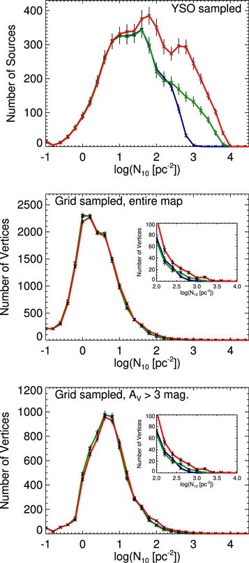
Figure 4. Nearest neighbor surface density PDFs for Orion A showing the effect of sampling and Av cutoff. The blue histograms give the densities for the dusty YSOs determined by Spitzer data alone, the green give the densities from Spitzer data corrected with Chandra data, and the red gives the Spitzer and Chandra data corrected for incompleteness (Megeath et al. 2016).
Download figure:
Standard image High-resolution imageThe YSO sampled PDFs for three nearby clouds, Taurus, Ophiuchus and Orion A, are shown in Figure 5. These show a several order of magnitude spread in the surface densities of YSOs, from a few stars per pc2 to almost 10,000 per pc2. The combined PDF of all the clouds within 500 pc covered by the c2d, Gould Belt and Orion surveys is also shown (using data from the SESNA program for the c2d and Gould belt regions, Evans et al. 2009; Megeath et al. 2012; Dunham et al. 2015; R. A. Gutermuth et al. 2022, in preparation). The combined surface density distribution of the nearby star-forming regions was first examined by Bressert et al. (2010). They found that the combined PDF has a lognormal form with a peak of 22 stars pc−2 and a dispersion of  . A caveat to their approach was that, due to the incompleteness in the Orion Nebula, they excluded the inner regions of the ONC. When included, the distribution deviates from a lognormal distribution with a tail at high densities (see Figure 5 and Kuhn et al. 2015b).

Figure 5. YSO sampled PDFs for the spatial distribution of dusty YSOs in Orion A, Ophiuchus, and Taurus molecular clouds. The different colors show the PDFs resulting from the three different completeness corrections applied to the Orion A data, as described in Figure 4.
Download figure:
Standard image High-resolution imageBressert et al. (2010) interpreted the lack of a discontinuity in the composite PDF as evidence against distinct clustered and distributed modes of star formation operating in these nearby clouds, with <26% of stars close enough to interact. Pfalzner et al. (2012) and Gieles et al. (2012) noted that such an interpretation was not unique. They showed that a superposition of multiple evolving clusters with different densities could reproduce the Bressert et al. PDF. Indeed, the PDFs of individual clouds show disparate PDF shapes, some dominated by high density clusters and others by low density distributed populations (Figure 5). Thus, the Bressert PDF does result from the superposition of multiple disparate PDFs.
Megeath et al. (2016) compared the PDFs of eight nearby molecular clouds. The clouds split into two distinct groups; the five clouds with clusters and median densities >25 YSO pc−2 and the three clouds without clusters and median densities below <10 YSO pc−2. Examples of these two groups are the Ophiuchus and Taurus molecular clouds (Figures 5 and 6); these clouds are at similar distances, have comparable masses, and contain similar numbers of dusty YSOs. Yet, in Ophiuchus most of the YSOs are concentrated in a single cluster while in Taurus, the YSOs are distributed throughout the cloud. This indicates the degree of clustering is not simply a function of the mass of a cloud or the number of YSOs. Instead, the density structure of the molecular cloud appears to be the most relevant factor (see Section 6.3).
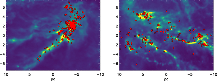
Figure 6. The distribution of YSOs in the Ophiuchus and Taurus molecular clouds. Left: Planck-derived extinction map of Ophiuchus with the YSOs from the SESNA processing of the c2d survey (Evans et al. 2009; R. A. Gutermuth 2022, in preparation). Right: Planck-derived extinction map of Taurus with the YSOs from Kenyon & Hartmann (1995). The coordinate scale is in parsecs at the distances of 130 pc and 140 pc for Taurus and Ophiuchus, respectively. The maps are from the Planck Legacy Archive (Planck Collaboration et al. 2014).
Download figure:
Standard image High-resolution imageWhile some clouds contain both clusters as well as diffusely distributed stars following the filamentary gas structure, others only have diffuse star populations. Based on these two distinct types of PDFs, Megeath et al. (2016) argued that 10 YSO pc−2 is an appropriate density threshold for identifying stars in clusters.
5. Star Formation Rate and Instantaneous Efficiency
The rate and efficiency are fundamental statistics that can characterize star formation on the scales of clouds and galaxies. The number and density of low mass YSOs, discussed in the previous section, provide a new means for measuring the rate and efficiency at which stars form throughout molecular clouds. These have been used by different authors to determine star formation relations in the clouds.
5.1. The Star Formation Rate (SFR)
The simplest estimate of the SFR is given by

where nYSO is the number of YSOs, tYSO is the lifetime of the YSOs in Myr, and m⋆ is the average mass for a typical IMF (0.5 M⊙). The value of nYSO is either the number of protostars (e.g., Heiderman et al. 2010; Lombardi et al. 2013) or the total number of dusty YSOs (e.g., Gutermuth et al. 2011), including both protostars and pre-main sequence (pre-ms) stars with disks.
When nYSO is the number of protostars, tYSO is the lifetime of protostars, ≈0.5 Myr (Dunham et al. 2014). If nYSO is the total number of dusty YSOs, then a lifetime for pre-ms stars with disks is required. The half-life of the disks is typically adopted for this lifetime, ≈2 Myr (Hernández et al. 2008; Evans et al. 2009; Mamajek 2009). The combined lifetime for protostars and pre-ms stars with disks, 2.5 Myr, can then be used for tYSO (Pokhrel et al. 2020).
One caveat to this approach is that tYSO may be affected by the local environment. The lifetime of protostars likely varies with their birth environment due to the dependence of the freefall times of the protostellar envelopes on the local gas properties. Evidence for this dependence is found by studies of protostellar luminosities, which find that protostars located in regions with high YSO densities (and therefore, high gas densities; see Section 5.3) exhibit systematically higher luminosities (Kryukova et al. 2012, 2014; Elmegreen et al. 2014). The higher luminosities likely reflect higher accretion rates, and therefore shorter protostellar lifetimes, in regions with high YSO and gas densities. This can result from shorter freefall times in the denser gas.
It is not clear whether the half-life of disks varies significantly with environment. The outer regions of disks are truncated by UV radiation from the surrounding environment, with the degree of truncation depending on the intensity of the radiation field (Adams et al. 2004; Mann & Williams 2010; Facchini et al. 2016; Haworth et al. 2017; Eisner et al. 2018; Petersen et al. 2019; van Terwisga et al. 2020). The effect of photoevaporation by UV on the inner regions of disks detected by Spitzer, however, is uncertain. Studies of clusters in the nearest 2 kpc have obtained mixed results on whether the lifetimes of the inner disks are shortened by the UV environment (Balog et al. 2007; Allen et al. 2012; Yep & White 2020). Thus, the SFR calculated from the total number of YSOs may be less dependent on environment than the SFR determined from protostars alone.
An alternative method for measuring the SFR uses the combined luminosities of protostars to calculate a total instantaneous accretion rate. This accretion rate is proportional to the total luminosity of the protostars. Adopting a typical mass to radius relationship, the SFR is given by the equation

where  is the luminosity of the ith protostar, m⋆/r⋆ is the mass–radius ratio, and η is the fraction of the accretion energy radiated into space. Since in most cases there are no direct measurements of η or the mass–radius ratios, values from models of protostars must be adopted (see Appendix A for details).
In Figure 7, we show the star formation rate calculated three different ways: using Equation (2) with the total number of YSOs in a given decl. bin (tYSO = 2.5 Myr), using Equation (2) with the number of protostars in that bin (tYSO = 0.5 Myr), and using Equation (3) with the total accretion luminosity for all the protostars in the bin. We find the answers can differ significantly. If we use Equation (2) and the total number of YSOs to measure the SFR, we find the peak SFR occurs in the Orion Nebula. If we instead use the total number of protostars, the peak is to the north of the nebula. Although there are biases against detecting protostars in the Orion Nebula, this analysis suggests that the star formation is currently concentrated north of the Orion Nebula, and the location of star formation has shifted northward. Furthermore, comparison to the SFR from Equation (3) suggests that using the standard protostellar lifetime (0.5 Myr) results in an underestimate of the current star formation rate. This implies that the protostars north of the nebula are accreting at a higher than typical rate. The inconsistencies between these methods motivate future studies. Methods for measuring the SFR with protostars require a deeper understanding of protostellar lifetimes and accretion. Furthermore, resolving differences between methods which measure the time averaged rate and those that measure the instantaneous rate require an understanding of the time dependency of the SFR.
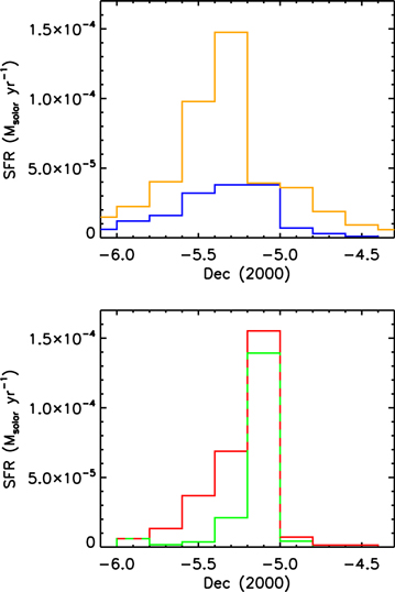
Figure 7. The SFR in the ISF (Figure 3). Each bin shows the total rate in that decl. range. Top: the yellow histogram is the SFR calculated from the total number of YSOs and the blue line is that calculated from the number of protostars, both using Equation (2). Bottom: the SFR calculated using the luminosities of the protostars and Equation (3); the green histogram has only the HOPS protostars while the red histogram includes a correction for protostars not observed by Herschel. See Appendix A.
Download figure:
Standard image High-resolution image5.2. The Star Formation Efficiency (SFE)
The instantaneous SFE is the fraction of the total mass that is found in stars,

where M⋆ is the current total mass in stars, Mcloud is the current molecular gas mass of the cloud, m⋆ is the mean stellar mass for a standard IMF, typically 0.5 M⊙, and nYSO is the number of YSOs. By directly counting the stars that constitute the bulk of the stellar population in both mass and number, this provides a direct and statistically robust measurement of the efficiency. For more distant regions, the efficiency is determined by indirectly measuring the number of massive stars (e.g., Lee et al. 2016). Although these approaches produce larger, more representative samples, they require more assumptions, are sensitive to statistical variations in the properties of the most massive stars, and cannot measure SFEs of smaller clouds without massive stars.
The determination of the SFE requires a measurement of the cloud mass, which is derived from near-IR extinction maps, molecular line maps, or thermal dust emission maps (see overview in Ridge et al. 2006). This mass does not include gas dispersed by winds, outflows and radiation, and the measured SFE can be increased by the clearing of gas by feedback.
We show the SFEs for entire clouds and for clusters in Figure 8. For the molecular clouds, the number of YSOs is that for the entire cloud and the mass is the total cloud gas mass. The adopted gas mass varies with the size of the survey field and the chosen gas tracer (e.g., C18O versus 13CO) since most of the mass is in the extended, low density gas (e.g., Schneider et al. 2015; Pokhrel et al. 2016). The SFEs of clusters require cluster boundaries to determine the number of YSOs (see Section 6). The gas masses have been determined by the virial masses of clumps coincident with the clusters (Lada 1992) or by the masses obtained by integrating column density maps over the regions subtended by the clusters (e.g., Megeath et al. 2016).

Figure 8. The instantaneous SFEs for clusters and clouds surveyed by Spitzer. Circular markers are clusters while square markers are clouds. Blue and red markers are from the Orion A and B clouds, respectively (Megeath et al. 2016), the light green makers are clusters from Gutermuth et al. (2009), and the dark green markers are clouds from Evans et al. (2009). For the Gutermuth et al. (2009) data, the cloud masses are determined by integrating 2MASS AV maps over the convex hulls determined for each cluster. The Orion cluster gas masses are also determined by integrating the 2MASS AV maps over the region subtended by the cluster (Megeath et al. 2016). For the cluster data and the Orion clouds, the number of dusty YSOs has been divided by 0.75 to correct for diskless pre-ms stars (Megeath et al. 2016). The dense core SFE is that estimated by Könyves et al. (2015).
Download figure:
Standard image High-resolution imageFigure 8 shows a picture apparent since the first IR cloud surveys (Lada 1992). Molecular clouds have a median SFE of only 0.038, with Orion B showing an unusually low SFE (0.0055). Clusters show a median SFE of 0.13, although with significant scatter. This scatter may arise from some clusters being at the onset of SF, and therefore gas rich, while other clusters are depleted of gas by star formation and the associated feedback. In the case of the highest mass cluster, the ONC, the high SFE may result from an overestimate in nYSO from completeness corrections and an underestimate of the gas mass by the AV maps due to the inability of 2MASS to penetrate the high extinction in parts of this cluster (Megeath et al. 2016). Finally, estimates for individual molecular cores give a value of around 0.40 for the SFE (e.g., Könyves et al. 2015). Thus, there is a factor of three increase in SFE from cloud to cluster scales, and another such increase from cluster to core scales.
The almost order of magnitude spread in the SFEs of the molecular clouds in Figure 8 may be due to cloud evolution. The observed SFE of a cloud will increase with time, rising first as gas is converted into stars, and then later due to the dispersal of the molecular gas. Thus, the instantaneous SFE will first underestimate and later overestimate the integrated SFE of a cloud, i.e., the total fraction of gas converted into stars over the lifetime of a cloud. This can lead to a large spread in the values of the observed SFEs for an ensemble of clouds even if the integrated efficiencies are similar (Grudić et al. 2019).
5.3. SF Relations in Molecular Clouds
Spitzer YSO surveys have uncovered star formation (sf-) relations within individual molecular clouds; arguably one of the most important and unexpected results from these surveys. These relations were motivated by observations showing that the local densities of YSOs and SFRs in molecular clouds vary by three orders of magnitude (Figures 5 and 7). These variations must result, at least in part, from variations in the gas environment from which the stars form.
A growing body of work indicates that gas density is the primary environmental factor. Comparisons of nYSO to the masses of clouds suggested that star formation occurred primarily in regions where the gas column and volume densities exceeded a threshold (AV ≥ 7 or n(H) ≥ 104 cm−3, Heiderman et al. 2010; Lada et al. 2010; Kainulainen et al. 2014). Subsequent work comparing the spatially varying surface density of YSOs, ΣYSO, to the corresponding column density of gas, Σgas, revealed a star-gas surface density correlation,

where, x, y is the position in a cloud and m ≈ 2. (Gutermuth et al. 2011; Masiunas et al. 2012; Lada et al. 2013; Lombardi et al. 2013; Rapson et al. 2014). This correlation is interpreted as a sf-relation within clouds,

where κ is a constant (Gutermuth et al. 2011). Here ΣYSO is calculated from the density of dusty YSOs (Gutermuth et al. 2011; Pokhrel et al. 2020) or from the density of protostars (Lombardi et al. 2013).
The sf-relation is apparent when the stellar and gas surface densities are smoothed over 0.2–1 pc scales (Gutermuth et al. 2011). Observations sampling <0.2 pc spatial scales begin to resolve individual dense cores. Sokol et al. (2019) found that dense cores are present even in regions where the smoothed gas surface density is low. They also found that the number of cores per area correlates with the column density of gas smoothed over 0.2–1 pc scales. Since these cores will collapse into individual stars (or stellar systems), this correlation likely gives rise to the observed sf-relation.
Initial measurements showed that m varied between 1.5 and 4 across an assortment of clouds. One of the primary uncertainties in this intra-cloud sf-relation is the effect of evolution and gas dispersal on the star-gas correlation. Pokhrel et al. (2020) mitigated this uncertainty by using the pre-ms star/protostar ratio as a proxy of age to exclude more evolved regions in a cloud. Using Herschel 160–500 μm data to map the column densities of gas in clouds, they found star-gas surface density correlations with m = 1.8–2.3 in twelve nearby clouds with gas masses ranging from 3000 to 1.8 × 10⁶ M⊙ (Figure 9). This value of m implies that the local instantaneous SFE increases approximately linearly with Σgas (Gutermuth et al. 2011), and thus provides a basis for understanding variations in the SFE from cloud to cluster scales.

Figure 9. The YSO surface densities vs. gas column densities for six molecular clouds surveyed with Spitzer and Herschel. These plots, adapted from Pokhrel et al. (2020), show densities measured at the positions of protostars in regions where the C ii/C i (i.e., pre-main sequence star/protostar) ratios are <30; this eliminates regions where gas dispersal has altered the correlation. The value of m are given for each cloud.
Download figure:
Standard image High-resolution imageThe scaling factor κ of the star-gas correlation varies from cloud to cloud (Lada et al. 2013; Pokhrel et al. 2020). Thus, this sf-relation only applies within a given molecular cloud and is not directly relatable to star formation relations found on galactic scales (Kennicutt & Evans 2012; Lada et al. 2012).
5.4. The Efficiency per Free Fall Time
The SFR can also be expressed as the fraction of molecular gas that is converted into stars per freefall time, or efficiency per freefall time,

where τff is the freefall time for the gas and tSF is the interval over which star formation has occurred. Since τff ∝ ρ−0.5, a typical gas density ρ must be determined. The efficiency has been calculated for dense clumps and entire molecular clouds, giving typical values of a few percent (e.g., Krumholz & Tan 2007; Lee et al. 2016).
Pokhrel et al. (2021) calculated the efficiency per freefall time for the clouds in their 2020 study, using the gas mass within successive gas column density contours to estimate the density (see also Evans et al. 2014). Using the number of YSOs within the surface density contours, they found that the intra-cloud sf-relation can be expressed as

where ΣYSO is the number of protostars in a gas surface density contour divided by the projected area of that contour, τff is calculated from the density estimated within a contour, and  ff is the star formation efficiency per freefall time. Due to its linear nature, Σgas and ΣYSO can be recast in terms of volume densities.
They found that for clouds within 1.5 kpc of the Sun, ff ≈ 0.026; this value decreases to ff ≈ 0.01 if corrections for the cloud structure are applied to the freefall time (Hu et al. 2021). The variation in efficiency between clouds are small: ![$\sigma [{\mathrm{log}}_{10}({\epsilon }_{\mathrm{ff}})]=0.2$](https://content.cld.iop.org/journals/1538-3873/134/1034/042001/revision1/paspac4c9cieqn5.gif) . Since this relation is found in clouds both with and without high mass stars, Pokhrel et al. (2021) suggest that star formation must be regulated, at least in part, on local scales by processes such as MHD turbulence, magnetic fields and protostellar outflows (e.g., Krumholz & McKee 2005; Hennebelle & Chabrier 2011; Padoan & Nordlund 2011; Federrath & Klessen 2012; Federrath 2015; Guszejnov et al. 2021).
. Since this relation is found in clouds both with and without high mass stars, Pokhrel et al. (2021) suggest that star formation must be regulated, at least in part, on local scales by processes such as MHD turbulence, magnetic fields and protostellar outflows (e.g., Krumholz & McKee 2005; Hennebelle & Chabrier 2011; Padoan & Nordlund 2011; Federrath & Klessen 2012; Federrath 2015; Guszejnov et al. 2021).
6. Characterizing Embedded Clusters
Near-IR surveys of molecular clouds in the 1990s showed that most low mass stars formed in embedded clusters (e.g., Lada et al. 1991; Ali & Depoy 1995; Carpenter 2000; Allen & Davis 2008). Spitzer and Chandra, with their ability to identify isolated YSOs, showed that these clusters are typically density peaks in populations of YSOs that extend across clouds (Figures 6 and 10, Allen et al. 2007).

Figure 10. Distribution of dusty YSOs in the Orion A molecular cloud. The black dots are isolated YSOs, the colored dots show the different clusters and groups extracted by Megeath et al. (2016), and the outline traces the extent of the Spitzer fields. The background image is the N(H2) map from Stutz & Kainulainen (2015). The ONC is the large cluster at the northern tip of the cloud marked in red.
Download figure:
Standard image High-resolution imageMultiple approaches have been developed for isolating clusters. The ONC provides an example where many of these approaches have been applied to a single cluster. Both Carpenter (2000) and Megeath et al. (2016) use non-parametric approaches for isolating the ONC, searching for contiguous regions of high YSO surface density that exceed a threshold density. The resulting cluster included most of the integral shape filament (ISF), contains ∼2000–3000 YSOs, and spans a 10 pc interval along the ISF (see Figures 3 and 10).
Parametric approaches have also proven fruitful. Hillenbrand et al. (1998), Da Rio et al. (2014), and Stutz (2018) fit a King model, a r−2.4 power-law, and Plummer sphere to the ONC, respectively. They focused on the central density peak of the cluster, which contains 1000 M⊙ in the inner 0.7 pc (Figure 3, Stutz 2018). Kuhn et al. (2014) decomposed the ONC into four isothermal ellipsoids. The primary ellipsoid has a half width of 0.31 × 0.16 pc and contains 834 members; within the boundaries of this ellipsoid are two ellipsoids tracing smaller density peaks. A fourth, highly elongated ellipsoid (0.23 × 0.04 pc) is located to the north of the other three ellipsoids and extends along the ISF. These disparate solutions show that results from different approaches must be compared with care.
6.1. Cluster Demographics
Adopting a method for identifying clusters, we can assess whether most stars form in large clusters, smaller clusters or groups, or isolation. Using the Spitzer catalog of dusty YSOs in the Orion clouds, and adopting a threshold density of 10 YSOs pc−2 for clusters (see Section 4.1), Megeath et al. (2016) found 17 groups with 10–100 members, three clusters with 100–1000 members, and one cluster, the ONC, with ∼2000 members (Figure 10). Similar to the pre-Spitzer result of Carpenter (2000), they found the largest clusters in a cloud contained more stars than all the smaller clusters combined.
Binning the number of YSOs into logarithimic decades of cluster size, they found that in both clouds, the bin containing the most massive clusters contained ≥60% of the YSOs, while each of the lower bins contained ≤20% of the YSOs. Again, for the Orion A and B clouds considered together, the ONC, which is the only ≥1000 member cluster in the clouds, contained ∼50% of the YSOs. Those in assemblages with <10 members were considered isolated; these constituted ∼20% of the YSOs. Thus the vast majority of stars form in clusters or groups.
This result for local clouds is in tension with extragalactic studies that show for bound clusters, the total mass of stars per logarithmic decade of cluster size is approximately constant (e.g., Larsen 2009; Fall & Chandar 2012). The lack of agreement is not surprising since many embedded clusters may dissolve or lose members due to gas dispersal as they become bound clusters (see Section 6.7). Furthermore, extragalactic samples include clusters formed from many different clouds within a galactic disk. Finally, the clusters detected in other galaxies are more massive than those typically found near the Sun. Nonetheless, the analysis of Megeath et al. (2016) should be extended to a larger sample of clouds to ensure that the Orion results are representative of clouds within 2 kpc of the Sun.
6.2. Cluster 2D Structure
Once a cluster has been extracted, its structural properties can be ascertained using the 2D spatial distribution of YSOs. Figure 11 displays the properties of clusters within 1 kpc taken from Gutermuth et al. (2009), Kuhn et al. (2015b) and Megeath et al. (2016). See Appendix C for a discussion on how these properties are determined. As discussed below, the trends in Figure 11 imply that the properties of the embedded clusters are largely set by their formation in their parental gas structures.
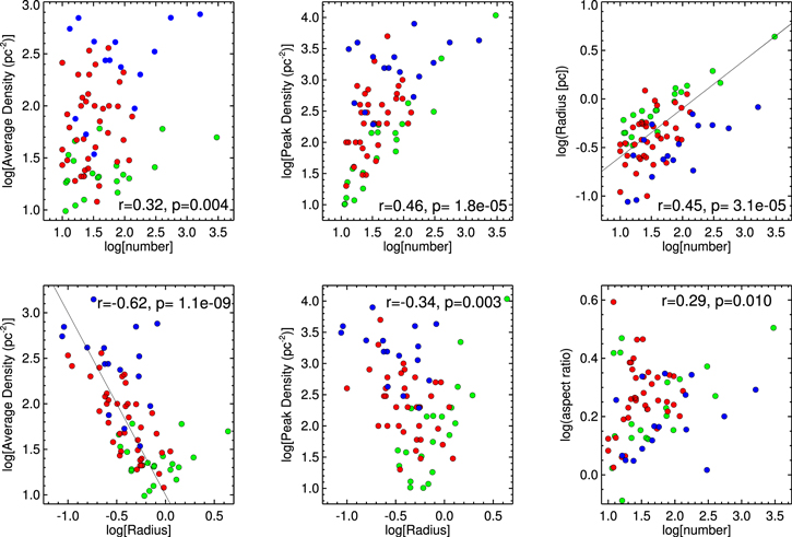
Figure 11. Cluster properties for Spitzer and Chandra surveys of clusters; green dots are clusters and groups in Orion from Megeath et al. (2016), red dots are cluster cores from Gutermuth et al. (2009), and the blue dots are sub-clusters from Kuhn et al. (2014). While there is no overlap between the Megeath et al. (2016) and Gutermuth et al. (2009) sample, the ONC is found in both the Megeath et al. (2016) and Kuhn et al. (2014). The line in the radius vs. number plot (upper right panel) is for a constant density of 64 pc−2 while the line in the density vs. radius plot (lower left panel) is for the density = 10/radius2.
Download figure:
Standard image High-resolution imageThe average surface densities of clusters depends on the extraction method. The clusters of Megeath et al. (2016) have densities near the adopted surface density threshold, the isothermal ellipsoids of Kuhn et al. (2014, 2015b) show higher densities, and the cluster cores of Gutermuth et al. (2009) fall in between. These systematic differences are also apparent in the average surface density versus radius plot, which shows an inverse correlation between density and radius. The isothermal ellipsoids and cluster cores often trace compact, high density structures hierarchically nested within large, lower density clusters (Kuhn et al. 2014). In a sample of clusters out to distances of several kiloparsecs, Kuhn et al. (2015a) found that the volume densities of ellipsoids decreased as the number of members increased. They suggested that the small, dense sub-groups merged and dynamically relaxed into larger, lower density clusters. The observed inverse correlation between density and radius likely reflects this process.
In contrast, there is a strong correlation between the peak density of a cluster and the number of members. Megeath et al. (2016) find a correlation of  where Npeak is the peak density and nYSO is the number of members. Megeath et al. (2016) also note that the mass of the most massive member also correlates with this density. There is no correlation of the peak density with radius. If the radius was determined by expansion, the peak density should decrease with increasing radius. These relationships thus indicate that the radii and densities of embedded clusters are determined primarily during their formation, and not by the subsequent evolution of the clusters.
A strong correlation is also found between cluster radius and the number of members. If we assign each member an average mass, a mass versus radius relationship of M ∝ R2 is consistent with the correlation in Figure 11. An analysis by Pfalzner et al. (2016) found a slightly shallower relationship for clusters of M ∝ R1.7. A similar relationship is found for cluster-forming molecular clumps, suggesting that the correlation is inherited from the properties of the parental dense gas structures (Pfalzner et al. 2016).
Finally, we find that all clusters with more than 60 members are elongated with aspect ratios ranging from 1.4 to 3, the most extreme example being the ONC. Smaller clusters show a wide range of aspect ratios; much of this scatter may be due to the larger uncertainties for these clusters. An alternative measure of the asymmetry is the azimuthal asymmetry parameter (AAP) of Gutermuth et al. (2005), which uses variations in the number of sources in pie shaped wedges centered on a cluster's center to establish azimuthal asymmetry. Megeath et al. (2016) use the AAP to show that all the Orion clusters with more than 100 members are asymmetric. Smaller clusters and groups may also be asymmetric, but lack the number of sources needed to have AAP values that deviate significantly from a symmetric cluster. The elongation is inherited from the morphology of the parental dense gas structures (Section 6.3).
6.3. The Gas Environment of Clusters
In Section 5, we found that the structures of clusters appear to be strongly influenced by their formation as opposed to their subsequent evolution. A deep connection between gas environment and cluster properties is also implied by the sf-forming relation discussed in Section 5.3. This relation shows that a continuum of stellar densities, rates and efficiencies are present in molecular clouds, and that clustered and diffuse star formation are the extremes of this continuum. Regions of a cloud with high column densities of gas form stars rapidly and produce embedded clusters with high SFEs. In the low column density regions that dominate the surface area of a cloud, a diffuse population of stars is formed at a low SFE. Given the typical gas column density PDFs of molecular clouds (e.g., Lada et al. 2013), and the concentration of high density gas in massive structures, most YSOs form in embedded clusters as discussed in Section 6.1.
Despite this continuum, there are distinct differences in the structure of the dense gas found in clusters and in areas of diffuse star formation. Figure 12 compares two regions of the Mon R2 cloud. The northern region contains the Mon R2 cluster. Here, the dense gas is organized into a hub with filaments extending outward radially, i.e., a hub-filament system (Myers 2009). The YSOs are concentrated in the central hub, which is elongated. In contrast, the low column density southern region shows a network of filaments with widths of ∼0.1 pc; these are similar to the filaments found in Herschel observations of many nearby clouds (e.g., Arzoumanian et al. 2019). The concentration of gas into filaments reconciles the low average density of this region with the requirement for pockets of the dense gas needed to form stars; accordingly, the observed protostars are found in the filaments. Due to its stronger gravity, much higher gas densities are attained in the hub, resulting in the high density of YSOs (Pokhrel et al. 2016). Both the high and low density regions have a mixture of protostars and pre-ms stars with disks, indicating that star formation has been sustained over several generations.
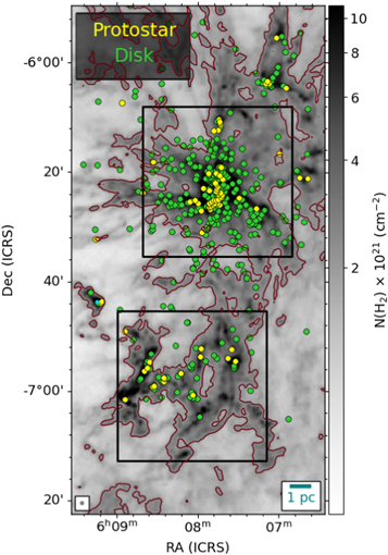
Figure 12. The distribution of YSOs and gas in the Mon R2 molecular cloud. The YSOs are from the SESNA survey (Gutermuth 2022, in preparation) and the gas is derived from Herschel dust continuum imaging of the cloud. The boxes outline two regions studied by Pokhrel et al. (2016); the upper region contains the rich Mon R2 cluster and the lower contains a diffuse star-forming region.
Download figure:
Standard image High-resolution imageEmbedded clusters are found in hubs, like that in Mon R2, or ridges. Ridges are massive, highly elongated counterparts to hubs (Motte et al. 2018); the 4000 M⊙ ISF, which hosts the 2000 member ONC, is the nearest and best studied example of a ridge (Figure 3, Bally et al. 1987; Megeath et al. 2016; Stutz & Gould 2016; Kong et al. 2019). The column density PDFs of both massive hubs and ridges show shallow power-law tails extending to N(H2) ≈ 1023 cm−2; these tails indicate the presence of high gas densities due to gravitational contraction (Ballesteros-Paredes et al. 2011; Stutz & Kainulainen 2015; Pokhrel et al. 2016; Kuznetsova et al. 2018). These tails suggests that hubs and ridges come from the collapse of cloud structures, with ridges resulting from the collapse of triaxial structures into massive filaments (e.g., Lin et al. 1965). Millimeter line observations show evidence for flows of gas, both radially contracting onto ridges and hubs and along the filaments that radiate from these structures (Schneider et al. 2010; Kirk et al. 2013; Rayner et al. 2017). These flows can supply gas to the hubs and ridges and sustain star formation. As is the case for the ISF, hubs and ridges are also the sites of high mass star formation (Hill et al. 2011; Kumar et al. 2020; Anderson et al. 2021).
Despite their elongation, ridges appear to be distinct from the narrow filaments that thread more diffuse star-forming regions and more similar to hubs (Hill et al. 2011; Hennemann et al. 2012). Their mass-to-length ratios are higher than those of filaments; the ISF has a mass to length to ratio of 390 M⊙ pc−1 within a radius of 1 pc from the spine of the ridge (Stutz & Gould 2016). Both ridges and hubs can have complex inner structures (Kainulainen et al. 2017; Hacar et al. 2018). Ridges also exhibit different radial density profiles than filaments. The density profiles of filaments show an inner flattening with a characteristic width of 0.1 pc and power-law volume density profiles of q = −2 (ρ ∝ rq ) at larger radii (Arzoumanian et al. 2019). In comparison the profiles of the ISF shows no flattening down to scales of 0.04 pc and a comparatively shallow q = −1.6 power-law density profile (Stutz & Gould 2016). Even for cross sections that include the density peak of the ONC cluster, Stutz (2018) find that the gas mass of the ISF dominates over the stellar mass of the ONC beyond 1 pc. The high gas density and shallow density profile provides the conditions necessary for the formation of parsec scale clusters like the ONC.
As discussed in Section 6.2, the properties of clusters are inherited from the structure of the dense gas. The elongated clusters align with the morphologies of the hubs and ridges in which they form (e.g., Figure 3, also Gutermuth et al. 2005). Pfalzner et al. (2016) show that the mass versus radius relationship for clusters is similar to that found for molecular clumps with massive stars by Urquhart et al. (2014); these clumps are likely to be distant hubs or ridges in our galaxy. The increase in the peak stellar density with the number of members (Figure 11) reflects the increasingly high gas column densities present in successively more massive hubs and ridges. The increase in the highest gas column densities with cluster size can be seen in the gas column density PDFs for the cluster-forming hubs in Mon R2. This can be seen by comparing the PDFs for regions 2 (smallest cluster), 4 (GG12-15, an intermediate mass cluster), and 8 (Mon R2, the most massive cluster) in Figure 13 of Pokhrel et al. (2016).
6.4. Tracing Fragmentation in Clusters
The density of star formation in clusters depends on the spatial distribution of fragmentation sites. The distribution of sites is determined, in turn, by the internal structure of hubs and ridges. In the Herschel dust continuum maps of the L1688 hub, Ladjelate et al. (2020) find a network of 0.1 pc diameter filaments similar to those in more diffuse regions. Using velocity integrated C18O line maps from CARMA, Suri et al. (2019) also resolved the ISF into a network of ∼0.1 pc diameter filaments.
An alternative approach is to use the position and velocity information in C18O or N2H+ molecular line maps to map dense gas structure. Hacar et al. (2013, 2016, 2018) decomposed the L1495 hub, the NGC 1333 cluster hub in the Perseus cloud, and the ISF, respectively, into spatially and kinematically coherent, highly elongated structures called fibers. The linewidths of the fibers are transonic, with the non-thermal components of the line profiles less than the sound speed (Hacar et al. 2018). The fibers in L1495 and NGC 1333 have widths of ∼0.1 pc; the ISF's fibers are narrower with widths of 0.02–0.05 pc (Hacar et al. 2018). The narrow widths may be due to the use of a specific dense gas tracer, N2H+, to map the fibers in the ISF (also see Figure 15).
The observed spatial distribution of pre-stellar cores in clouds, i.e., those that are unstable to collapse, shows that the fragmentation of the dense gas preferentially occurs in the filaments and fibers. Herschel dust continuum maps of the cluster forming Ophiuchus, Perseus and Serpens clouds (spatial resolution ≤0.07 pc) show that within the hubs/ridges, >80% of the pre-stellar cores are found in filaments (Ladjelate et al. 2020; Fiorellino et al. 2021; Pezzuto et al. 2021).
Filaments and fibers containing cores typically have mass-to-length ratios ≥8 M⊙ pc−1, similar to or in excess of the ratio for a stable, gravitationally bound isothermal filament (16 M⊙ pc−1). This is consistent with these structures being unstable to radial collapse and/or fragmentation (Pezzuto et al. 2021).
Hacar et al. (2018) find that fibers mapped in the N2H+ line, a dense gas tracer, contain cores and conclude that these fertile fibers are unstable to fragmentation. They show that the number of fertile fibers per surface area scales with the overall mass-to-length ratio of their host structure; with the density of fibers increasing between the filaments of Taurus and the massive ISF ridge. In this picture, the primary difference between cluster forming and diffuse regions is the surface density of fertile fibers.
The fragmentation scale, as measured by the separations between protostars or between cores, is comparable to the thermal Jeans length (Teixeira et al. 2006, 2016). It is, however, the rate a which the gas fragments into cores that primarily determines the rate of star formation in a cluster. An estimate of the rate can be obtained by extending the results of Pokhrel et al. (2018). They examined the fragmentation of the Perseus molecular cloud at each step of its structural hierarchy: from cloud to clumps, to cores, to envelopes and finally to protostars. Here the protostars are identified by VLA radio continuum surveys (Section 3.4), the envelopes are structures resolved inside the cores by SMA interferometric dust continuum maps, and the cores are found by single dish dust continuum maps of the cloud. The presence of multiple envelopes in a core or multiple protostars in an envelope imply multiplicity.
At each scale, Pokhrel et al. (2018) determined the number of Jeans masses, NJ = M/mJ, where M is the total mass in a structure and mJ is the Jeans mass calculated using the thermal sound speed. They then determined the efficiency of fragmentation, f
= N/NJ where N is the observed number of fragments, on cloud, clump, core, and envelope scales. The clumps are parsec scale structures that include hub-filament systems. Fragmentation of the clumps into cores has an efficiency of f
∼ 0.2.
If the cores collapse over a freefall time, then the rate of fragmentation is ≈0.2NJ/tff, where tff ≈ 2 × 10⁵ yr for the average volume density of the clumps. For the clump forming the NGC 1333 cluster, this implies a fragmentation rate of ∼120 per Myr. This is comparable to the rate of SFR from the YSO counts; about ∼70 per Myr assuming a protostar lifetime of 0.5 Myr (Gutermuth et al. 2009). The agreement is promising, particularly if a fraction of the cores do not collapse into stars or core lifetime exceeds a freefall time (Kirk et al. 2017; Sokol et al. 2019). Future studies can refine this approach through more detailed examinations of the gas structure at each level of the hierarchy, and the application of the analysis to other star-forming regions.
6.5. Age Spreads in Clusters
Clusters sustain star formation over a few million years until they disperse their natal molecular gas and star formation ceases. During this time, the number of protostars is proportional to the star formation rate smoothed over a protostellar lifetime. Over a few million years, the ratio of pre-ms stars with disks to protostars (also called the Class II/Class I ratio) increases to values of 4–6 for a constant rate of star formation, and then higher as the star formation rate and the number of protostars decreases (Appendix C). In Figure 13, we show the distribution of the ratios for the cluster cores in Gutermuth et al. (2009). The ratios range from 1.4 for a very young, protostar rich cluster, to 31 for more evolved clusters in the later stages of gas dispersal. In a simple model where all protostars have a fixed lifetime and disks disappear exponentially with a half life of 2 Myr (Mamajek 2009), these ratios require a period of sustained star formation that lasts 2–3.5 Myr, or about seven protostellar lifetimes (Appendix C). This conclusion depends on the adopted model for protostellar evolution. Assuming that protostars transition probabilistically into pre-ms stars with a fixed half life, Kristensen & Dunham (2018) find mean cloud ages of 1.2 Myr; these ages imply a shorter duration for cluster formation.
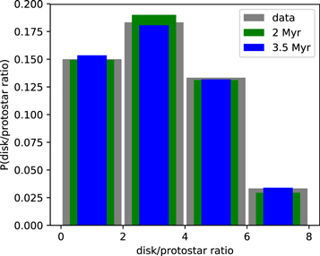
Figure 13. Normalized histogram of the ratio of the number of pre-ms stars with disks to the number of protostars in 36 cluster cores identified by Gutermuth et al. (2009). This is compared to simple models of cluster evolution with primary star formation episodes lasting 2 or 3.5 Myr. The histogram is reproduced if star formation is sustained over seven protostellar lifetimes in the cluster cores. See Appendix C.
Download figure:
Standard image High-resolution imageFor clusters where the members have effective temperatures and luminosities cataloged from a combination of photometric and spectroscopic observations, a comparison of the cluster HR diagram to theoretical pre-ms isochrones can determine ages and constrain star formation histories. The availability of accurate distances from Gaia has resolved one of the primary uncertainties in this method (e.g., Luhman et al. 2016; Ortiz-León et al. 2018b). Substantial debate has focused on the interpretation of scatter within the HR diagrams of individual clusters. This scatter was interpreted by Palla & Stahler (2000) as evidence for accelerating star formation rates in clusters, with the oldest stars having ages approaching 10 Myr. Hartmann (2001) argued that much of the scatter is due to uncertainties in the stellar luminosities caused by variability and multiplicity. In this case, the implied acceleration and age spreads are artifacts caused by the scatter. An analysis of the HR diagram of the ONC by Reggiani et al. (2011) showed that the uncertainties could not account for the full observed spread, and that the data are consistent with age spreads of 1.5–3.5 Myr, smaller than those originally proposed by Palla & Stahler (2000). Further evidence for age spreads of this magnitude is found in the spread of surface gravities and radii (Jeffries 2007; Reggiani et al. 2011; Da Rio et al. 2016). In aggregate, the disk to protostar ratios and the HR diagrams point to age spreads of a few million years.
Within these age spreads, there is evidence for spatial and temporal correlations. Beccari et al. (2017) and Jerabkova et al. (2019a) found evidence for distinct episodes of star formation in the ONC. Using visible-light CMDs and Gaia DR2 distances, they found evidence for two, potentially three, episodes of star formation occurring between 1.4 and 4.5 Myr ago. These episodes are extended along the ISF, with the youngest episode most concentrated toward the center of the ONC.
Spatial correlations may also be present in the form of age gradients. On >1 pc spatial scales, Pillitteri et al. (2013) combined IR and X-ray surveys to measure the ratio of stars without disks to stars with disks, or Class III to Class II ratio. This ratio increases with age. They found that the Class III to Class II ratio increases in the outer regions of the ONC. Thus, the outer regions contain older stars that either formed in previous star-forming episodes or migrated from the current region of active star formation.
On ≤1 pc scales, Getman et al. (2014) found radial age gradients in the ONC and NGC 2024 clusters, with the age again increasing with distance from the cluster center. Combining X-ray data and near-IR photometry, they used an X-ray luminosity versus mass relationship and pre-ms tracks to convert Lx and MJ, the X-ray luminosity and absolute J-band magnitude, of cluster members into an age, Agejx . For the two largest clusters in Orion, the ONC and the NGC 2024 cluster, they found gradients in the median Agejx as a function of cluster radius, with the ages increasing with radius. Consistent with this age gradient, they also found the fraction of YSOs with K-band excesses decreasing with increasing median Agejx . In a study of NGC 1333 and Serpens Main cluster, Winston et al. (2009) found similar gradients in the isochronal ages, with the fainter, older stars concentrated in the outer regions of the clusters. They found, however, that the Class III/Class II ratio did not show a corresponding gradient. They argued that the gradients in isochronal ages were spurious and resulted from the high extinction values found in the centers of clusters hiding the faintest stars, thereby biasing the median age to younger values in the centers. Resolution of these contrary claims require studies that address incompleteness in clusters.
In more evolved clusters, star formation can continue on their edges. In the IC 348 cluster, Muench et al. (2007) found protostars and a high rate of star formation on the edge of the cluster, while star formation in the center of the cluster has ceased due to gas dispersal. A similar configuration is found in the Cep OB3b cluster, where star formation continues on the edge of the eastern sub-cluster (Section 6.7, Getman et al. 2009; Allen et al. 2012).
6.6. The Kinematics of the ISF and ONC
The incipient motions of the stars in an emerging cluster are inherited from the parental gas. Ridges such as the ISF show complicated motions over a range of scales (Figure 14). These include turbulence (Li et al. 2013; Friesen et al. 2017), oscillations (González Lobos & Stutz 2019), gravitational infall (Hacar et al. 2017) and rotational motions (Álvarez-Gutiérrez et al. 2021; Hsieh et al. 2021).

Figure 14. Left: mass-to-length ratios for stars and gas along the ISF; this shows that the stars are strong concentrated near the center of the ridge, but the gas mass-to-length ratio only increases by a factor of 2–3 at this position. Right: intensity-weighted velocity centroids of the N2H+ (1–0) line along the ISF detailing the complex velocity structure of the filament. The x marks the center of mass and mean velocity of the ONC stars. Figure adapted from González Lobos & Stutz (2019).
Download figure:
Standard image High-resolution imageIn the ISF, the cores have motions that closely follow their parental dense gas (Stutz & Gould 2016), and these complex motions are important for understanding the kinematics of the nascent stars. Kong et al. (2019) compared the radial velocities of the cores in the ISF (measured with the dense gas tracer NH3) relative to the surrounding moderate density gas (traced by C18O). They found a local velocity dispersion of 0.35 km s−1 (Kong et al. 2019); this value is comparable to the sound speed of the gas and less than the velocity dispersion of the moderate density gas of the ISF, ∼0.5 km s−1. This velocity dispersion is also less than the virial velocity estimated for the filament following the analysis of Fiege & Pudritz (2000), 0.8 km s−1. Other regions show similarly small core velocity dispersions relative to the surrounding gas (Walsh et al. 2004, 2007).
A velocity dispersion can also be calculated from the observed core velocities. This core to core velocity dispersion is sub-virial in the NGC 1333 cluster of the Perseus cloud (Walsh et al. 2007; Foster et al. 2015) and the L1688 cluster in the Ophiuchus cloud (André et al. 2007). Due to the complex gas motions in the ISF, however, the global core to core velocity dispersion in the ISF is 2.9 km s−1, much higher than the estimated virial velocity. Thus, locally the motions of the cores are sub-virial relative to their natal gas, but on the scale of a cluster, the core to core velocity dispersion can be super-virial due to the complex motions of the parental ridge or hub inherited by the cores.
As stars form, they decouple from the dense gas from which they collapsed. The 350 μm dust continuum map in Figure 15 shows the dense gas structures in the OMC2/3 region of the ISF; these structures closely follow the N2H+ emission used to identify fibers (compare to Figure 3 of Hacar et al. 2018). Overlaid are the protostars separated into three different SED classes. These classes correspond approximately to a succession of evolutionary stages, although with some ambiguity due to the inclinations of the protostars (Furlan et al. 2016). The youngest objects, the Class 0 protostars, are coincident with the dense gas structures. The intermediate aged Class I protostars show a mixture of sources on and off the structures. Most of the oldest protostars, the flat spectrum sources, are displaced from the structures. This successive detachment of the protostars from the dense gas may be driven by a combination of several factors: the accretion of the dense gas onto the protostars, the dissipation of the structures by feedback or turbulent motions in the surrounding gas, and the slingshotting of protostars out of the structures due to the acceleration of the gas (e.g., Stutz & Gould 2016; Osorio et al. 2017).
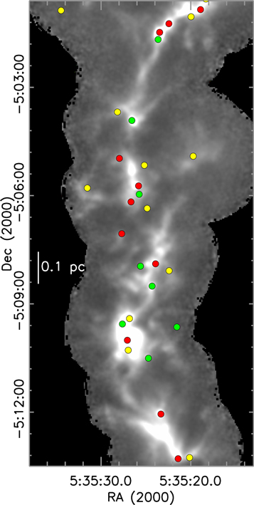
Figure 15. Distribution of protostars in the OMC2/3 region of the ISF. The grayscale shows the APEX/SABOCA 350 μm map of the dense gas structure (T. Stanke 2022, private communication). The Class 0 (red), class 1 (green) and flat spectrum (yellow) protostars are overlaid (Furlan et al. 2016).
Download figure:
Standard image High-resolution imageAfter stars inherit the velocities of their natal cores, their motions are determined by the combined potential of the ISF and ONC and occasional flybys of other members. For the kinematics of the ONC as a whole, the global, super-virial core to core velocity dispersion may be more relevant. This high velocity dispersion may explain why pre-ms stars in the ONC are spread out in R.A. and are no longer concentrated in the dense backbone of the ISF along with the protostars (Figure 3).
One of the most distinctive features in the PV diagram of the ISF is a gradient in radial velocity north of the center of the ONC (Figure 14). The velocities of the stars, cores and gas become increasingly blueshifted with decreasing projected distance to the center (Tobin et al. 2009; Kounkel et al. 2016; Hacar et al. 2017; Kong et al. 2019). The gradient has been interpreted as the acceleration of the gas and stars in the ISF by the concentration of mass at the cluster center (Peterson & Megeath 2008; Tobin et al. 2009; Hacar et al. 2017), or as the result of wave-like oscillations in the ISF (Stutz & Gould 2016; Stutz et al. 2018).
In the case of acceleration, the resulting motion would produce a mass infall onto the center of 50 M⊙ in gas per million year (Hacar et al. 2017). This interpretation requires that the ISF is inclined such that the center of the ONC is closer to the Sun than the filament to the north. Gaia DR2 parallaxes for the infrared, visible, and X-ray selected YSOs in the ISF suggest that the center of the ONC is more distant than the filament on either side (Stutz et al. 2018; Getman et al. 2019; Kuhn et al. 2019).
For this inclination, the velocity gradient implies that gas is moving away from the center of ONC. The correlated variation of the gas radial velocity and Gaia DR2 derived distance along the ISF has been interpreted as evidence for a wave-like oscillation (Stutz et al. 2018; Kong et al. 2019). Given the scatter in the parallaxes and the inability of Gaia to detect stars deeply embedded in the ISF, however, the inclination of the ISF remains uncertain.
The density of stars is strongly peaked within 0.3 pc of the center of the ONC, which is located in the Orion Nebula where the most massive stars are found (Figures 14, 2, Hillenbrand & Hartmann 1998). Although the ONC is highly elongated, the elongation decreases with increasing stellar density and disappears within 0.1 pc of the peak; this may be the result of dynamical relaxation (Megeath et al. 2016). Inside the central 0.3 pc, proper motions measured in the near-IR with HST and Keck (Kim et al. 2019) and in the radio with the VLA (Dzib et al. 2017) show no evidence of expansion, rotation or contraction while Gaia DR2 data (Kuhn et al. 2019) shows a marginal detection of expansion. The velocity dispersion is, to good approximation, Gaussian and increases toward the center of the cluster (Kim et al. 2019; Theissen et al. 2022). When including the gas mass inside the cluster, as estimated from the extinction to the member stars (Da Rio et al. 2014), the velocity dispersion is marginally super-virial (Da Rio et al. 2017; Kim et al. 2019; Theissen et al. 2022).
Although this central cluster of the ONC may be dynamically evolved and bound, there are four reasons why it will not be in a stable equilibrium over timescales of 1–2 Myr, i.e., the relaxation time of the central 0.1 pc (Megeath et al. 2016). First, toward the center of the ONC where the stellar mass is concentrated, the gravitational acceleration perpendicular to the ISF by the gas exceeds that from the stellar mass at distances greater than 0.36 pc (Stutz 2018). The O-star θ1C Ori, which appears to be at the center of the cluster, is offset by 0.1–0.2 pc from the ionization front at the surface of the ISF (Wen & O'dell 1995; O'Dell et al. 2017). Thus the ISF and central cluster are spatially offset. Accordingly, the cluster is likely being pulled and tidally stretched by the cloud (Stutz 2018).
Second, the velocity dispersion along the filament is 25% higher than that perpendicular to the filament: σv
α
= 1.64 ±0.12 km s−1 and σv
δ
= 2.03 ± 0.13 km s−1 (Jones & Walker 1988; Kim et al. 2019; Kuhn et al. 2019; Theissen et al. 2022). This higher velocity dispersion may result from stars falling into the cluster potential and contributing to the elongation of the cluster. Third, the velocity dispersion in the line of sight, i.e., toward the filament, is even higher:  km s−1 (Theissen et al. 2022). Tidal acceleration by the filament may have inflated velocities in this direction (Stutz 2018). This velocity dispersion exceeds the virial velocity from Da Rio et al. (2014). Furthermore, due to the tidal force of the filament, a higher mass may be required for virial equilibrium (Lee & Rood 1969). The fourth and final reason is that the gas potential is changing on 1–2 Myr timescales due to gas dispersal and possible motions in the filament (Stutz 2018, see Section 6.7).
Another source of change is the ejection of stars. In the ONC, >50 candidate members have been ejected within the last 4 Myr with velocities of >6 km s−1, most of which trace back to the innermost Trapezium region at the cluster center (McBride & Kounkel 2019; Farias et al. 2020; Schoettler et al. 2020). The most massive star in the cluster, θ1 Ori C has likely played a role in a large fraction of these ejections. Almost all of these runaway and walkaway stars tend to be low mass; such stars are more abundant and it is easier to accelerate them. Only two O stars, μ Col and AE Aur, are known to have been ejected from the vicinity of the ONC in an event 2.5 Myr ago (Hoogerwerf et al. 2001). In general, the mass loss due to ejection is only a few percent of the total mass. The ejection of OB stars, however, may alter cluster evolution by reducing feedback on the surrounding cloud (e.g., Kroupa et al. 2018).
6.7. The Effect of Gas Dispersal
Feedback from the member stars is thought to be the primary means by which clusters lose their gas and star formation halts (e.g., Hartmann et al. 2001). Since the molecular gas dominates the masses of embedded clusters (Section 5.2), the dispersal of the gas should have a large impact on the evolution of the clusters (e.g., Hills 1980). Understanding the evolution of clusters through gas dispersal has implications for a range of astrophysical inquiry, from the the evolution of planetary systems (e.g., Adams 2010) to the use of clusters to trace star formation in other galaxies (e.g., Krumholz et al. 2019).
By comparing the rate of formation of embedded and bound open clusters, Lada & Lada (2003) estimated that only 7% of embedded clusters survive gas dispersal to become bound clusters. With censuses of open clusters and YSOs around the Sun provided by Gaia and Spitzer, respectively, we can estimate the fraction of all stars formed that remain bound in clusters after gas dispersal (Kruijssen 2012). Anders et al. (2021) identified all open clusters in a 2 kpc radius cylinder centered on the Sun. From the masses and ages of the clusters, they estimated the rate of open cluster formation in units of mass is  M⊙ Myr−1 kpc−2. From the total number of YSOs in the Orion clouds plus all clouds within 500 pc, the local star-forming rate is 1700 ± 22 M⊙ Myr−1 kpc−2. Thus, in the local region of our galaxy,
  of stars emerge from their birth clouds in bound open clusters. If open clusters come from the 65% of stars that form in ≥100 member embedded clusters (Adams & Myers 2001; Megeath et al. 2016),
  of all stars that form in such embedded clusters emerge in open clusters. See Appendix D for details.
N-body simulations of cluster evolution during gas dispersal initially assumed that the stars and gas have similar spatial distributions and are initially virialized (e.g., Lada et al. 1984). These models found that the fraction of stars that remain in bound clusters depend on the integrated SFE and the rate of gas dispersal. In the case of rapid gas dispersal, Baumgardt & Kroupa (2007) found that integrated SFEs ≥ 33% are needed for clusters to survive. Alternatively, when the removal of the gas occurs over multiple crossing times, clusters with efficiencies as low as 10% survive.
Motivated by simulations of cluster formation in turbulent clouds that predicted sub-clusters dominated by stellar mass with sub-virial stellar velocities, subsequent work predicted that most clusters survive rapid gas dispersal (e.g., Goodwin 2009; Kruijssen et al. 2012; Farias et al. 2018). Furthermore, based on comparisons of clump masses to the properties of young massive clusters, conveyor belt models were proposed in which gas steadily flows into the central cluster as the stellar population grows (Longmore et al. 2014; Walker et al. 2016). The hierarchical structure, sub-virial velocities and conveyor belt flows increases the fraction of stars that remain bound and the chances that clusters with low integrated SFEs survive.
In contrast, models incorporating feedback show that irregular shells of gas swept up by winds and radiation from massive stars can accelerate young stars; this process can help disperse clusters (Zamora-Avilés et al. 2019). These theoretical developments motivate a detailed examination of the process of gas dispersal. While the nearest 1 kpc lacks the sample size of studies of more distant regions in our galaxy and others, it does host specific examples that can be studied in detail. The remainder of this section concentrates on these examples.
Observations are now directly measuring the effect of the OB stars in the ONC on the ISF (Figure 16). SOFIA [C ii] maps trace a 1500 M⊙ neutral hydrogen shell expanding at 13 km s−1 (Pabst et al. 2019). This shell is part of a 0.2 Myr old bubble driven by the wind of the O7 star θ1 Ori C, which is in center of the Orion Nebula. The shell is apparent in Figure 3 as a large arc of nebulosity that extends to the southwest of the nebula. The other two bubbles surround B-stars and appear to be driven by the expansion of the hot, ionized gas (Pabst et al. 2020). One of these bubbles surrounds the NGC 1977 sub-cluster at the northern tip of the ISF (Figure 3, Peterson & Megeath 2008). The age of this bubble is 0.4 Myr. These observations show that gas dispersal starts at multiple locations along a ridge driven by either winds or H ii regions.

Figure 16. Integrated 158 μm [C ii] map of the ISF from the upGREAT instrument on SOFIA (Pabst et al. 2019). The O and B stars from Brown et al. (1994) are the large and small star markers, respectively. The Orion nebula and Trapezium are at the center. This image shows the massive 1500 M⊙ bubble extending southwest from the Trapezium, the bubble around the B-stars in NGC 1977 to the north, and the small bubble around a single B-star in M43 just northeast of the center.
Download figure:
Standard image High-resolution imageIs the ONC forming a bound cluster? The most likely part of the ONC to survive gas dispersal is the central cluster, i.e., the stars within 0.3 pc of the center. This high stellar density region appears to be undergoing relaxation (Megeath et al. 2016). The massive stars in this central region drive the wind bubble detected in [C ii] observations. The age of this bubble, 0.2 Myr, is similar to the crossing time of the central 0.3 pc of the cluster, indicating that the dispersal of the gas is rapid (Baumgardt & Kroupa 2007; Pabst et al. 2020).
Although the velocity dispersion of stars in the cluster slightly exceeds the virial velocity, the cluster shows no signature of contraction and only a weak signature of expansion (Section 6.6). The stellar and gas masses in the central 0.3 pc are approximately equal, suggesting a SFE ∼ 50% (Figure 14). This does not include, however, the gas in the 1500 M⊙ wind bubble (Pabst et al. 2020). If the swept up gas started in the inner parsec, then the SFE at the onset of gas dispersal may have been closer to 30%.
The large bubble driven by θ1 Ori C is filled with YSOs, including protostars, that are displaced from the spine of the ISF (Figure 3). These stars may have formed in the gas as it was accelerated leaving a trail of young stars behind, or they may have been accelerated by the gravitational pull of the expanding, inhomogenous bubble (Zamora-Avilés et al. 2019). There are hints that these stars are expanding away from the ONC in the kinematic data (Fűrész et al. 2008; Getman et al. 2019). These data suggest that the expansion of some of the stars is driven by feedback sweeping up the molecular gas. The bulk of the stars in the core of the cluster, however, remain unaffected.
In aggregate, these observations suggest the central 0.3 pc of the ONC is on the cusp of forming a few hundred solar mass bound cluster (Baumgardt & Kroupa 2007; Farias et al. 2018), although the effect of the filament on the cluster remains unclear (Section 6.6). Continued star formation in the filament will increase the size of the eventual bound cluster (Otter et al. 2021). This star formation may potentially be fed by molecular gas falling into the central 0.3 pc (Section 6.6), similar to the flows invoked in conveyor belt models.
Other embedded clusters show approximately virial velocity dispersions for stars. Foster et al. (2015) found that while the cores in the NGC 1333 cluster have a sub-virial velocity dispersion, the stars and the gas have velocity dispersions that are comparable to the virial velocity for the total star and gas potential (Figure 17). In addition, the gas density exceeds the stellar density on all spatial scales (Foster et al. 2015). Gaia proper motions of NGC 1333 show no evidence of rotation or expansion (Ortiz-León et al. 2018b). Similarly, the pre-stellar cores in L1688 also have a sub-virial velocity dispersion (André et al. 2007). The stars in this cluster once again have a virial velocity dispersion for the combined star and gas potential (Rigliaco et al. 2016). These examples demonstrate that the young stars in clusters can achieve virial velocity dispersions before gas dispersal. Since both of these clusters have instantaneous SFE of 30% (Gutermuth et al. 2009), it is likely both will survive to form bound clusters (Baumgardt & Kroupa 2007; Farias et al. 2018).

Figure 17. Velocity dispersions of cores, stars and gas within a maximum radius max from the center of the NGC 1333 cluster. These are compared to the virial mass calculated from the total stellar and gas mass enclosed within Rmax; this virial mass does not include terms for magnetic fields or external pressure (Foster et al. 2015). The plot shows that cores have a sub-virial distribution while the stars appear virialized. Figure from Foster et al. (2015).
Download figure:
Standard image High-resolution imageIf the stars in embedded clusters have approximately virial velocity dispersions in a potential that is dominated by the gas, then the dispersal of the gas should lead to the expansion of the clusters. Indirect evidence for expansion is found in the densities and structures of clusters. In a study of three clusters, Gutermuth et al. (2005) show that two embedded clusters are elongated and aligned with their parental hubs and ridges, while the third cluster, which has dispersed much of its gas, has a lower stellar density and no elongation. They propose that the lower density and circular symmetry of the third cluster is due to its expansion after gas dispersal from a denser, elongated initial configuration.
Kinematic evidence for expansion is less clear. The IC 348 cluster in Perseus is in the late stages of gas dispersal, with the central cluster largely cleared of gas (Muench et al. 2007). IC 348 shows a super-virial velocity dispersion relative to the stellar mass (Cottaar et al. 2015). It also shows, surprisingly, evidence that the stars on the near and far side of the cluster are converging; this is interpreted as either two converging sub-clusters or the cluster oscillating around a new equilibrium radius in response to gas dispersal (Cottaar et al. 2015). Yet, Gaia DR2 data of IC 348 show no evidence of rotation and expansion (Ortiz-León et al. 2018b).
In the nearest 1 kpc, the strongest evidence for expansion due to gas dispersal is found in Cep OB3b, a massive, ONC sized cluster in the later stages of gas dispersal which contains two distinct sub-clusters (Figure 18, Allen et al. 2012). The smaller western sub-cluster contains B-stars. Its relatively low density indicate that this sub-cluster has expanded due to gas dispersal. Despite this expansion, the radial velocities suggest that the emerging cluster is bound (Karnath et al. 2019).
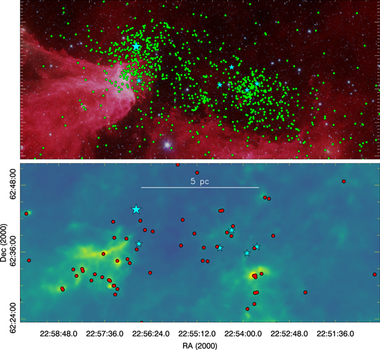
Figure 18. The spatial distribution of YSOs in the Cep OB3b cluster. The top panel shows the Spitzer 3.6, 4.5 and 8 μm combined image with the locations of the pre-main sequence stars with disks displayed (Allen et al. 2012, data from SESNA). The bottom image is a N(H2) column density map of the remnant molecular cloud (Pokhrel et al. 2020) with the location of protostars overlaid (also from SESNA). The protostars that are not coincident with gas structures are likely to be edge-on disks or extragalactic contamination (Kryukova et al. 2012). The location O and B stars are shown as large and small star markers, respectively (Allen et al. 2012). The 5 pc bar shows the approximate length of the ISF shown in Figure 3; this cluster has a similar number of members to the ONC but is in the late stages of gas dispersal.
Download figure:
Standard image High-resolution imageIn contrast, the more massive eastern sub-cluster (also referred to as Cep B, e.g., Getman et al. 2006) hosts an O7 star. Its radial velocity dispersion suggests that this sub-cluster is on the whole unbound, although there are large uncertainties due to multiplicity (Karnath et al. 2019). Gaia DR2 astrometry of this sub-cluster shows expansion with a magnitude consistent with the radial velocity dispersion (Kuhn et al. 2019). The relatively low surface density and circular symmetry of the sub-cluster are also indicative of expansion (Karnath et al. 2019).
The most massive stars in the Cep OB3b sub-clusters appear to influence the fraction of stars that survive gas dispersal in bound clusters. Comparing the virial ratios of the sub-clusters to the results of N-body codes, Karnath et al. (2019) argue that both sub-clusters will form bound clusters with ∼300 members. In the larger eastern sub-cluster, which hosts an O-star, only a relatively small fraction of members remain bound (Farias et al. 2018). In contrast, in the western sub-cluster, which is undergoing slower gas dispersal by B-stars, a large fraction of members remain bound. Averaging Gaia DR2 proper motions, Karnath et al. (2019) find that the two sub-clusters are moving apart to form a double cluster.
Pang et al. (2020) find a possible 25 Myr analog to Cep OB3b using Gaia DR2: the double cluster NGC 2232 and LP 2439. While both are expanding, the smaller NGC 2232 appears to be bound and undergoing re-virialization, while only half the members of the larger LP 2439 are bound. Like the eastern sub-cluster of Cep OB3b, LP 2439 probably underwent rapid gas dispersal and may ultimately dissolve while the lower mass cluster survives.
Although the current number of examples are small in number, they point to a picture where clusters become virialized before the gas is dispersed. Gas dispersal then leads to super-virial velocity dispersions and expansion, but the clusters can survive the loss of gas in a bound state. This is often accompanied with a significant loss of stars (e.g., Weidner et al. 2007). The ONC will likely lose the lower density regions outside the central 0.3 pc (Figure 3), while the eastern sub-cluster of Cep OB3b will lose more than half its stars due to its globally unbound state (Karnath et al. 2019). Clusters with slower gas dispersal, such as the western sub-cluster of Cep OB3b, lose a smaller fraction of stars. Although these (sub)-clusters survive gas dispersal, subsequent dynamical evolution, stellar evolution, or tides may disrupt them (e.g., Kruijssen 2012; Moeckel et al. 2012; Domínguez et al. 2021).
Gas dispersal will also affect the merging of sub-clusters. In a study of 28 clusters and associations in our galaxy, Kuhn et al. (2019) use Gaia DR2 to show that in cases where there are multiple sub-clusters in a region, they are moving away from each other and will not merge. As is the case for Cep OB3b, the sub-clusters have dispersed much of their parental gas. Kuhn et al. (2019) argue that if merging occurs, it must happen during an earlier embedded phase when gas dominates the mass.
7. Clusters and Associations
The clusters and molecular clouds discussed in previous sections are often parts of larger complexes of stars and clouds. The ISF, which contains the ONC, is part of the Orion A molecular cloud, a highly elongated, filamentary cloud that extends 90 pc in length (Figure 10, Bally et al. 1987; Großschedl et al. 2018). Orion A, in turn, is part of the Orion Complex which extends for almost 200 pc and contains multiple generations of stars that have formed over the last 12 Myr in a succession of epochs (Briceno 2008; Kounkel et al. 2018). This complex contains the Orion OB1 association, whose massive stars power a superbubble 400 pc in diameter (Bally 2008; Ochsendorf et al. 2015).
Complexes contain a mixture of low and high mass stars located both in molecular clouds and in large populations that have dispersed their natal clouds. While low mass stars in the molecular clouds can be identified by the presence of dusty disks and envelopes, coronal X-ray emission, or compact clusters, identifying the low mass stars outside of clouds is more difficult. These older stars have low disk fractions, are dispersed over areas too large to efficiently survey at X-ray wavelengths, and often require time consuming spectroscopic measurements (Briceño et al. 2007; Hernández et al. 2007). For these reasons, the full extent of many complexes have historically been traced by their massive stars and referred to as OB associations (de Zeeuw et al. 1999).
With the release of Gaia DR2 and EDR3 and systematic spectroscopic surveys such as APOGEE-2, it is now possible to identify and characterize the populations of low mass stars outside of the clouds using the 6D data obtained by combining their positions in the sky with parallaxes and 3D motions. In the Orion complex, which includes the Ori OB1 association, Kounkel et al. (2018) used 6D data to identify 10,000 low mass members in the complex. They find that the entire complex is co-moving, with a velocity dispersion of a few km s−1. This indicates a common origin. The densest regions of the association are the clusters embedded in the molecular clouds; yet the lower density off-cloud population shows considerable spatial and kinematic structure (Figure 19, Kounkel et al. 2018).

Figure 19. The young stars in the Orion molecular cloud complex and OB1 association plotted over an Av map from the Planck Legacy Archive (Planck Collaboration et al. 2014). The red dots are the young stars either from the Spitzer survey (Megeath et al. 2012, 2016) or from Gaia DR2 (Kounkel et al. 2018). Also shown are the O stars (large blue circles) or B stars (small blue circles) of the Orion OB1 association (Brown et al. 1994). The coordinates are parsecs at a distance of 400 pc. The map is oriented in galactic coordinates: the ONC is centered near X: 10 pc and Y: 5 pc.
Download figure:
Standard image High-resolution imageThe nearby Sco OB2 association also shows significant spatial structure as well as a diffuse population that contains most of the stars (Preibisch & Mamajek 2008; Wright & Mamajek 2018). The densest regions of the association are the embedded cluster in the Ophiuchus cloud (Figure 6) and an isolated off-cloud peak; it is not known if this peak is a bound cluster (Röser et al. 2018; Damiani et al. 2019). Proper motions show most of the association is unbound, with asymmetric velocities dispersions and complex kinematic sub-structure (Wright & Mamajek 2018; Damiani et al. 2019).
In a Gaia DR2 study of 109 galactic OB associations,Ward et al. (2020) find substantial kinematic sub-structure. They rule out models where the associations arise from the expansion from one or several clusters. Their model of the observed motions requires several distinct components including one with random velocities, sub-structures with correlated velocities, and expansions from multiple clusters (also see Wright et al. 2016). Looking back at the stellar distribution of the Orion A cloud (Figure 10), the spatially correlated components may arise from the small groups/clusters along the filament of the cloud; as shown by Kounkel et al. (2018), these stars exhibit complex kinematics that include a large velocity gradient along the filament. The expanding cluster could come from the dense center of the ONC. These components will merge into the association as the Orion A cloud disperses. The Gaia DR2 analysis of Kuhn et al. (2019) finds expanding clusters in several associations.
With Gaia DR2 and EDR3, it is possible to identify distinct populations of stars in the Orion complex (Kounkel et al. 2018; Chen et al. 2020), as well as use the observed trajectories of the stars to infer dynamical evolution. Many of the observed trajectories indicate infall. Several clouds, as well as a number of small populations of young stars that have already dispersed their gas, are moving inward toward the complex's center of mass. The most massive of these clouds is the Orion B cloud. On smaller scales, the σ Ori cluster, the densest, post-gas dispersal cluster in the complex, is moving toward the Orion B cloud (Kounkel et al. 2018).
Extreme expansions are also observed in the Orion Complex. The observed expansions are ballistic, and given their magnitude (>6 km s−1), may be attributed to the shockwaves of two supernovae sweeping away the molecular gas and triggering star formation in the process (Großschedl et al. 2021; Kounkel 2020). One of them dates back ∼4 Myr within the λ Ori cluster. The other one dates back ∼6 Myr, likely originating along the sightline near η Ori at the geometrical center of Barnard's loop. This supernova has been responsible for shaping much of the morphology of the Orion Complex. Given its location, the gas swept up along its shock front may have led to the formation of the ONC, the most massive cluster in the solar neighborhood (for a different view on these motions, see Swiggum et al. 2021).
The properties of associations result from several factors. First, associations form in complexes of elongated and filamentary clouds that can extend over 100 pc in length: the Orion A and B clouds span the diameter of the Orion complex (Figure 19, Megeath et al. 2016). The overall size of the association is mostly determined by the size of the complex and not by expansion.
Second, associations are assembled primarily from the embedded groups and clusters that form in the clouds, and they inherit the velocity structure of the gas. The stars from the groups and clusters expand and/or disperse into the association creating complex kinematic and positional sub-structure. Infall motions and expansions driven by massive feedback add to the complex kinematic structure.
Third, star formation is sustained in associations for ∼10 Myr, longer than the ages of individual clusters or clouds (Section 6.5, Hartmann et al. 2001), in a patchwork of star-forming regions that come and go through time (Zari et al. 2019; Wright 2020). In nearby associations such as Orion, massive star formation appears to have occurred throughout this ∼10 Myr interval (Wright 2020). This is in tension with results from extragalatic studies that find cloud lifetimes of 10–30 Myr with the massive stars and H ii regions appearing in only the last 1–5 Myr (Kruijssen et al. 2019; Chevance et al. 2021).
Finally, due to the large spatial extent of the molecular cloud complexes, associations are assembled over regions where the crossing time, as calculated with the stellar velocity dispersions in localized sub-regions such as the ONC (∼50 Myr for a ∼2 km s−1 velocity dispersion), is much longer than the star-forming time in a cloud (∼3.5 Myr) or association (∼10 Myr) (Hartmann et al. 2001; Wright 2020). Within an association, embedded clusters form with crossing times less than their lifetimes; these may survive and remain bound after the association disperses (Gieles & Portegies Zwart 2011).
All young populations are slowly dissolving into the field as they age. However, because an individual molecular cloud tends to form several hundred to a few thousand stars, and because their original dispersion velocity mirrors that of the clouds and is much lower than the field distribution, they persist as comoving groups. In recent years, with the improved ability to identify such comoving stellar populations afforded by Gaia, a number of older structures have been found (Jerabkova et al. 2019b; Kounkel & Covey 2019; Beccari et al. 2020). Many of these populations are string-like configurations that extend in length on average 200 pc and have widths of only ∼10 pc (Figure 20). They are unlikely to have formed by tidal stretching of clusters, or associations significantly more compact than their current dimensions, as such lengths are observed in strings of all ages from <10 to >100 Myr. Rather, they resemble the shapes of filamentary molecular clouds from which they likely formed (Zucker et al. 2018), and they are well-matched by the typical dimensions observed in the molecular clouds (Zucker et al. 2018). Some, but not all, strings contain star clusters. Only a few young star clusters exist in isolation without extended stellar populations surrounding them. This shows that most clusters formed as parts of filamentary clouds.
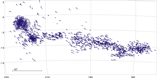
Figure 20. Distribution of members of a ∼20 Myr old stellar string associated with the cluster NGC 2232. The plot is in the galactic coordinates. Arrows how the proper motions of the stars in the local standard of rest. Members were identified in Kounkel et al. (2020), see also Tian (2020).
Download figure:
Standard image High-resolution imageAs more and more comoving populations with different ages have been identified, it is now possible to determine statistics about their survivabillity. Kounkel & Covey (2019) find that most strings persist up to ages of ∼200–300 Myr, comparable to the orbital time of the Sun around the Galaxy. Beyond that age, the remaining comoving groups are typically compact and isolated—potentially remnants of the densest cluster-like environments that have formed inside of a cloud, while the rest of the diffuse population has largely been dispersed. Nonetheless, it is also possible to find a few stellar strings up to the ages of a few Gyr. These strings tend to be much more diffuse than their younger counterparts, with only a few dozen stars remaining. They are likely the surviving remnants of the populations that were the most massive at the time of their formation. Overall, the number of stars in a population that remains comoving as a function of age, regardless of size or mass, can be characterized by the relation

where No is the typical number of stars found in a population with an age of 10 Myr, and t is the age of the population in years (Kounkel & Covey 2019).
8. Summary
In Section 2, we introduced four questions in the current study of star formation. In this review, we addressed these questions using surveys of low mass YSOs combined with studies of the associated molecular gas. Here we summarize our current progress in answering these questions, and suggest future lines of inquiry.
Question: What are the rates, densities and efficiencies of star formation in molecular clouds, and how much do they vary with environment?
- 1.Young low mass stars and protostars, or YSOs, are important tracers of star formation on cluster and cloud scales. Over the last 20 yr, surveys at X-ray, visible, IR and radio wavelengths have detected, identified, and characterized populations of YSOs in many clouds in the nearest 1.5 kpc. The resulting catalogs of YSOs are the basis of wide ranging investigations into star and cluster formation (Section 3).
- 2.The surface densities of YSOs measured in clouds within ≤500 pc of the Sun range from 0.1 to 104 pc−2. The combined, YSO sampled PDF of these clouds is approximately lognormal for low to moderate densities, peaks near 20 pc−2, but has a distinct wing at higher densities primarily due to the rich clusters found in Orion (Section 4.1).
- 3.Within individual molecular clouds, comparisons of the surface densities of YSOs to column densities of gas show power-law star-gas correlations in regions without significant gas dispersal, where
 (Section 5.3).
 - 4.The spatially averaged, instantaneous SFE varies from ∼4% for entire molecuar clouds to ∼13% for clusters, although with large scatter. This is consistent with the star-gas correlations which imply that the instantaneous SFE within a cloud varies linearly with the surface density of gas until a significant fraction of the gas is expelled by feedback (Sections 5.2 and 5.3).
- 5.The SFR can be measured from the number of dusty YSOs and adopted lifetimes of disks and protostars, or from the total luminosities of protostars. Inconsistencies between these approaches remain unresolved (Section 5.1).
- 6.The star-gas correlations can be interpreted as a sf-relation where the SFR per area scales as the square of the gas column density. These correlations can also be reproduced by a sf-relation with a constant SFE per freefall time of ≈0.01–0.03 (Sections 5.3 and 5.4). Question: What are the differences between diffuse and clustered star formation, and how do they depend on cloud properties?
- 7.Several techniques are used to extract clusters from 2D maps of YSOs, with notable differences between the results. Cluster extraction applied to cloud surveys shows that clouds contain multiple assemblages, ranging in size from small groups to massive clusters. In clouds with clusters, the most massive clusters contain approximately half the stars while ∼20% of the YSOs are relatively isolated (Sections 6 and 6.1).
- 8.Due to the sf-relations in clouds, clusters form in regions with high gas column densities and are observed as peaks in the stellar density. Thus, clustered and diffuse star formation are a continuum that is a function of the density of gas. The SFE per freefall time sf-relation varies little between clouds forming massive stars and low mass stars, showing that it does not depend on the feedback of massive stars (Sections 6.3, 5.3 and 5.4).
- 9.The PDFs of individual clouds vary significantly. Clouds without clusters have median densities <10 pc−2 while those with clusters have median densities >20 pc−2. The presence of clusters is determined by the structure of the dense gas in a cloud (Section 4.1).
- 10.Clusters form in hubs and ridges while diffuse star formation occurs primarily in networks of filaments with 0.1 pc diameters. Hubs are massive concentrations of molecular gas that appear at the intersections of multiple filaments. The filaments can supply hubs with flows of gas as the hubs form stars. Ridges are much more elongated than hubs, and have higher mass to length ratios and different radial density profiles than filaments (Section 6.3).
- 11.Hubs and ridges contain significant substructure that have been characterized as filaments (using 2D intensity maps) or as fibers (using 3D position–velocity data); these structures appear to be the sites of fragmentation. The density of unstable fibers/filaments may correlate with the density of star formation, with the highest densities found in clusters (Section 6.4). Question: What is the duration of cluster formation, and during this time, what processes shape the structure and kinematics of clusters?
- 12.Based on the observed ratios of the number of pre-ms stars with disks to the number of protostars, star formation in clusters is sustained for approximately 2–3.5 million years, or about seven protostellar lifetimes. This time interval is also reflected in the age spreads in HR diagrams (Section 6.5).
- 13.There is evidence for spatial and temporal correlations of the SFR within clusters, both in the form of age gradients between the edges and interiors of clusters, and the presence of multiple, distinct episodes of star formation extending across a cluster (Section 6.5).
- 14.Structural analyses of the extracted clusters show a mass to radius relationship and a correlation between the peak YSO surface density and the total number of members. Clusters are also typically elongated. These correlations appear to be inherited from their formation in hubs and ridges (Sections 6.2 and 6.3).
- 15.YSOs inherit their velocities from the complex gas motions observed in hubs and ridges. Locally, the velocities of cores relative their natal gas appears sub-virial. The global core-to-core velocity dispersion, however, can be sub-virial or supervirial, depending on the region. In the ISF the global dispersion is supervirial due to the motions over the length of the ISF (Section 6.6).
- 16.The velocities of cluster members show that clusters are often dynamically evolved, neither expanding or rotating, and often have velocity dispersions close to the virial velocity. The presence of massive, nearby gas structures, asymmetries in the velocity dispersion, and rapid gas dispersal suggest, however, that clusters are not in equilibrium (Section 6.6).
- 17.Embedded clusters can lose mass through ejections. In the case of the ONC, the observed rate is small and will only reduce the cluster mass by a few percent. The rare ejections of massive stars, however, may have a large effect by changing the amount of feedback (Section 6.6). Question: How does star formation in cloud complexes produce a mixture of bound clusters and unbound associations, and how long do these assemblages persist in the galactic disk after star formation ends?
- 18.The SFR within 500 pc of the Sun is 1700 M⊙ Myr−1 kpc−2. A comparison of the rate at which open clusters form with this SFR finds that of stars emerge from their birth clouds in open clusters. If clusters are primarily formed from ≥100 member embedded clusters, then of the stars in embedded clusters emerge in open clusters (Section 6.7).
- 19.The cluster forming gas is removed by the expansion of H ii regions around early B stars or winds of O stars; these can occur at multiple locations along a ridge or hub. The gas dispersal is being mapped by observations of emission lines from PDRs with SOFIA (Section 6.7).
- 20.Since the velocity dispersions of the stars in embedded clusters are often close to the virial velocity for the star and gas potential, the loss of gas can have a large effect. Measurements of cluster surface densities and kinematics have found clusters expanding in response to the removal of their parental gas. Sub-clusters are observed to be moving apart and do not appear to merge to form larger clusters, in part due to the dispersal of the gas that binds them (Section 6.7).
- 21.There is some evidence that the rate of gas dispersal is important in the production of clusters, with clusters undergoing rapid dispersal by O-stars showing more rapid expansion and retaining only a relatively small fraction of their stars in a bound cluster. Clusters undergoing slower gas dispersal by B-stars may retain a much larger fraction of their stars (Section 6.7).
- 22.Clusters are typically found in large, filamentary molecular clouds, and these clouds are often parts of large complexes that can span 200 pc and sustain star formation for 10 Myr. Using Gaia and radial velocities, 6D observations of star formation complexes now trace the older, lower density stellar populations that have dispersed their natal gas and expanded (Section 7).
- 23.The kinematics of the associations of stars outside the clouds require that they are formed from multiple components. These components likely originate from a mixture of multiple clusters, smaller groups of stars, and more isolated stars that form in clouds. The stars within complexes also show both expansive motions due to supernovae, and inward motions which may be due to gravity (Section 7).
- 24.The stellar associations of embedded and post-embedded stars that span these complexes have crossing times, determined with local stellar velocity dispersions, that are much longer than the 10 Myr lifespans of the complexes. These associations, however, contain clusters of stars whose crossing times are less than their ages and can form bound clusters (Section 7).
- 25.Despite the complex motions, remnants of complexes can persist for up to 200–300 Myr. These remnants appear in Gaia observations of the local galaxy as string-like structures, many containing clusters (Section 7).


Future directions: The next few decades will bring new opportunities for extending surveys of low mass YSOs. JWST will survey dusty YSOs in more distant regions of our Milky Way, as well as the LMC and SMC, providing a more representative sample of star formation in our Galaxy and others. SDSS-V and the SKA will find young stars without requiring the presence of a disk or envelope. This capability will be further expanded by the ngVLA and future X-ray space telescopes.
A deeper understanding of protostellar and pre-ms evolution will improve measurements of the star formation rates and histories in clouds. Spectroscopic studies of protostars with JWST and near-IR spectrographs on large telescopes can measure accretion onto protostars and constrain their effective temperatures and radii, while ALMA can determine their masses. These data will provide strong observational constraints on protostellar accretion and evolution (e.g., Hartmann et al. 2016; Tobin et al. 2020b). Improved surveys for multiplicity, observational constraints on the initial conditions of pre-ms contraction, and a deeper understanding of the role of magnetic fields, rotation, and star spots in pre-ms evolution are needed to obtain robust ages and star formation histories in clouds and clusters (e.g., Binks et al. 2021; Cao et al. 2022; Serna et al. 2021).
Surveys of dense cores with both single-dish telescopes in nearby regions and ALMA in more distant regions will provide an independent means to study star formation rates and efficiencies (e.g., Sokol et al. 2019; Anderson et al. 2021). This includes using observations of cores to measure the rate of fragmentation or the efficiency of fragmentation per freefall time over the full range of cloud environments (Section 6.4). Such studies coupled with observations of turbulent motions, magnetic fields and outflows can guide models of how star formation is regulated in clouds (e.g., Burkhart et al. 2015; Pillai et al. 2020; Xu et al. 2022).
Even in the ISF, our understanding of the evolution of clusters during gas dispersal remains incomplete. Kinematic studies can be expanded to a larger number of clusters within the nearest 1–2 kpc that sample the full range of observed SFEs (Figure 8). Such studies will be performed with a combination of SDSS-V, Gaia, and potentially through proper motion measurements of embedded stars with the Roman space telescope. Observations of stars outside of clusters, many using Gaia, can estimate the fraction of stars in embedded clusters that are lost during gas dispersal (e.g., Weidner et al. 2007; Karnath et al. 2020; Heyl et al. 2021). Models of cluster evolution need to account for the continual formation of stars and feedback from those stars over multiple generations (Grudić et al. 2021; Guszejnov et al. 2021; Kim et al. 2021) and the gas motions in ridges that can inflate the velocity dispersion in clusters (e.g., Stutz & Gould 2016; González Lobos & Stutz 2019).
We thank Dr. Amelia Stutz for a careful reading and insightful comments on cluster kinematics. Dr. Riwaj Pokhrel supplied plots and expertise into star formation relations. Dr. Michael Fellhauer provided insights in cluster evolution during gas dispersal. Dr. Thomas Stanke produced the beautiful APEX/SABOCA 350 μm map of the OMC2/3 region. Sam Federman carefully read the text and gave numerous useful comments. Drs. Cornelia Pabst and Xander Tielens provided the [C ii] data cube from SOFIA. S.T.M. received funding from the NASA ADAP grant 80NSSC18K1564 and S.T.M., R.A.G. and M.A.K. received funding from the NASA ADAP grant 80NSSC19K0591. RAG also acknowledges funding support from: NASA ADAP awards NNX11AD14G, NNX13AF08G, NNX15AF05G, and NNX17AF24G; NSF AST grants 1636621, 1812747, and 2107705; NASA-USRA SOFIA grants 05-0181, 07-0225, and 08-0181; NASA-JPL/Caltech Spitzer grants 1373081, 1424329, and 1440160 and Herschel grant 1489384. During the completion of this review, S.T.M. was a Fulbright Scholar at the Universidad de Concepcíon, Chile; he thanks Dr. Amelia Stutz and UdeC for hosting him. Finally we thank an anonymous referee for their insightful comments and valuable suggestions, and the editorial staff of the PASP for their infinite patience. We acknowledge the extensive contributions of Dr. Judith Pipher, who helped develop the detector arrays for IRAC on Spitzer, and who - with her students - started an investigation into the sf-relations discussed here.
Appendix A: Calculating the SFR from the Integrated Protostellar Luminosity
In Section 5.1, we show a calculation of the SFR in bins of decl. along the ISF (Figure 7). One of the calculations used the integrated protostellar luminosity to get a total mass accretion rate, which is equal to the current SFR Equation (3). The displayed luminosity histograms were calculated using the bolometric luminosities of the HOPS protostars given by Furlan et al. (2016); due to extinction and inclination effects, the actual luminosities may be as much as a factor of two times higher. As protostars evolve, their accretion luminosities drop and their luminosities begin to be dominated by the intrinsic luminosities of the central protostars (Fischer et al. 2017). To limit the sample to protostars with accretion dominated luminosities, we require that they have Tbol < 100 K. Finally, we adopted η = 0.8 (this is the fraction of the accretion-generated energy that is radiated away as luminosity) and m⋆/r⋆ = 0.15 (see Fischer et al. 2017). The HOPS survey did not include the Orion Nebula region due to its bright nebulosity. To correct for this bias we used the protostars detected at shorter wavelengths in Megeath et al. (2012, 2016). To add in this contribution, we included all of the protostars in the nebula that were not included in HOPS. To determine the total accretion luminosity of these protostars, we first multiplied the number of non-HOPS protostars in each of the decl. bins coincident with the nebula by the fraction of HOPS protostars with Tbol < 100 K. We then multiplied the resulting number of protostars by the mean luminosity of the HOPS protostars. In Figure 7, we show the accretion rates with and without the correction for the missing protostars in the nebula.
Appendix B: Calculating Cluster Properties
In Figure 11, we combine the number of members, mean densities, peak densities and radii from three studies that have systematically extracted and characterized clusters in Spitzer and/or Chandra data. In this appendix, we summarize how these values were calculated. Kuhn et al. (2014, 2015b) fit isothermal ellipsoids plus a constant background to their distributions of X-ray and IR selected YSOs. As discussed in Section 6, multiple ellipsoids can be fit to a cluster like the ONC, and they are referred to in Kuhn et al. (2014) as sub-clusters. To determine the properties, we used the r4,major, r4,minor and nxlf values in Table 2 of Kuhn et al. (2015b). The first two values are the radii of the semimajor and semiminor axis for an ellipsoid with a radius four times the core radius, and nxlf is the number of members corrected for incompleteness using the XLF of each region. From these values, we calculated

where r, Nmean, Npeak and α are the radius, mean density, peak density and aspect ratio, respectively. In our analysis, we only use the clusters at distances ≤1 kpc; i.e., those sub-clusters associated with the ONC, W40, the Flame Nebula and the NGC 2264 regions.
Gutermuth et al. (2009) and Megeath et al. (2016) use different methods for extracting clusters from the distribution of IR selected YSOs, but once extracted, they use the same equations for determining the cluster properties. For each cluster, they determine a convex hull that contains the cluster, with each vertex being a cluster member; the area of this convex hull is Ahull. They also measure the minimum radius of a circle that contains the entire cluster, rcirc. Finally, they calculate the nearest neighbor density Nn for each member. The cluster properties are then given by
Megeath et al. (2016) use N10 to calculate the peak density while Gutermuth et al. (2009) use N6. In contrast to Kuhn et al. (2015b), these surveys only count YSOs with dusty disks and envelopes that can be identified in the Spitzer data. Furthermore, Gutermuth et al. (2009) do not apply any correction for incompleteness, while Megeath et al. (2016) apply a correction for incompleteness due to the bright nebulosity in Orion.
To extract the clusters, Gutermuth et al. (2009) construct a minimum spanning tree connecting the YSOs for each Spitzer field (e.g., Cartwright & Whitworth 2004). They rank the branches by their length and cut the branches longer than a critical branch length. This critical length corresponds to the transition from a rapid to slow increase in length with rank. They refer to the extracted structures as cluster cores. The cluster core properties are taken from their Tables 6 and 8. In contrast, Megeath et al. (2016) use a density threshold. They identify all sources with a Nn ≥ 10 pc−2; for all YSOs that satisfy the criteria, the 10 nearest YSOs that also meet this criteria are considered friends. Using a friends of friends analysis, they identify clusters of friends (see Figure 10). The cluster properties are given in their Table 2; we used the completeness corrected number, radius, aspect ratio and peak density from that table.
Appendix C: The Ratio of Disks to Protostars and the Star Formation History
To model the histogram of disk to protostar ratios for an ensemble of young clusters, we adopted a model SFR, ϕ(t), which starting at time 0 shows a linear rise to a maximum star formation rate at t0. The SFR plateaus at  between t0 and t1. Between t1 and t2 there is a linear decrease in the SFR to
  . After t2, the ϕ(t) drops exponentially with an e-folding time of t3. This is described by the equations


The protostellar stage is assumed to last for tproto, hence the number of protostars for a cluster with age tcluster is given by

After the protostellar stage, a star immediately transitions into a pre-ms star with disk. The optically thick disks detected by Spitzer disappear exponentially with time with a half-life of thalf (Mamajek 2009). Thus, the number of disks (i.e., Class II objects) at time tcluster is

Finally, after the optically thick disks disappear, the number of diskless stars (Class III objects) is

The SFR, Nproto, Ndisk, and Ndiskless are plotted as a function of t in Figure 21. To obtain the distribution of disk to protostar ratios, we assume that the observed cluster cores are uniformly distributed in tcluster between 0 and 10 Myr and that all the observed clusters have Ndisk ≥ 0.25Nproto; in other words, the youngest clusters are not included in our sample. We perform the calculations shown in Figure 21 for discrete values of tcluster separated by a constant time interval. We then plot histograms of the ratios of Ndisk to Nproto for all values of tcluster where Ndisk ≥ 0.25Nproto.
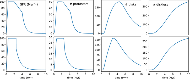
Figure 21. The two models used to calculate the distribution of ratio of pre-ms stars with disks to protostars in Figure 13. Each row shows one of our two model, with the adopted SFR and the resulting number of protostars, pre-ms stars with disks, and pre-ms stars without disks as a function of time.
Download figure:
Standard image High-resolution image
We find two solutions that reproduce the observed distribution. The first is where t0 = 0.5 Myr, t1 = 2 Myr, t2 = 4 Myr, and the exponential decay time is τ3 = 0.5 Myr (top row of in Figure 21). In this solution the protostellar lifetime, tproto is 0.5 Myr and the disk half life is tdisk = 2 Myr. In the second solution, t0 = 0.5 Myr, t1 = 2.5 Myr, t2 = 2.5 Myr, and the exponential decay time is τ3 = 0.75 Myr (bottom row in Figure 21). In this solution, we reduced the protostellar lifetime to tproto = 0.285 Myr and kept the same disk half life of tdisk = 2 Myr. In both cases, the primary star formation time, between the onset of the plateau and the end of the 33% drop in SFR, is seven times the protostellar lifetime.
Appendix D: The Star Formation Rate in the Nearest 500 pc
To compare the SFR in open clusters within a 2 kpc cylinder centered on the Sun, as estimated by Anders et al. (2021), to the current rate of SFR, we use the census of all dusty YSOs, i.e., protostars and pre-ms stars with disks, within 500 pc of the Sun. We restrict our estimate to this distance since our census of YSOs is much more complete in the nearest 500 pc. We assume that the SFR per galactic surface area in the nearest 500 pc is similar to that in the nearest 2 kpc.
We use the entire SESNA processing for the clouds within 500 pc to determine the number of YSOs in the Auriga, Cepheus Flare, Chameleon, Coronus Australis, Lupus, Musca, Ophiuchus, Perseus, and Scorpius clouds (Evans et al. 2009; Dunham et al. 2015; Pokhrel et al. 2020; R.A. Gutermuth et al. 2022, in preparation). The total number of dusty YSOs is 2953; after correcting for contamination of 9 objects per sq. deg. (Pokhrel et al. 2020), this value is 2624. We augment these using the Orion YSO catalog supplemented by Chandra X-say sources in the ONC and NGC 2024 described by Megeath et al. (2016); this is 3889 YSOs which drops to 3810 YSOs after correcting for contamination. The number of dusty YSOs in Taurus is 226 (Luhman et al. 2010). Finally, the number of dusty YSOs in the Pipe molecular cloud is 18 (Forbrich et al. 2009). Using these numbers and the equation

(see Section 5.1), we find that SFR = 1700 ± 22 M⊙ Myr−1 kpc−2 assuming Poisson uncertainties in the numbers of sources and contamination. The value in open star clusters is  M⊙ Myr−1 kpc−2. Propagating the uncertainties we find that the percentage of stars formed that emerge in clusters is
  . If we assume that only the 65% of stars that form in embedded clusters with 100 members or more can become open clusters (Megeath et al. 2016), then the fraction of those stars that emerge in open clusters is
  .
.