

Abstract
Astrometry at centimeter wavelengths using Very Long Baseline Interferometry is approaching accuracies of ∼1 μas for the angle between a target and a calibrator source separated by ≲1° on the sky. The BeSSeL Survey and the Japanese VERA project are using this to map the spiral structure of the Milky Way by measuring trigonometric parallaxes of hundreds of maser sources associated with massive, young stars. This paper outlines how μas astrometry is done, including details regarding the scheduling of observations, calibration of data, and measuring positions.
Export citation and abstract BibTeX RIS

Original content from this work may be used under the terms of the Creative Commons Attribution 3.0 licence. Any further distribution of this work must maintain attribution to the author(s) and the title of the work, journal citation and DOI.
1. Introduction
This paper focuses on the techniques of differential astrometry using Very Long Baseline Interferometry (VLBI) at centimeter wavelengths. Here I use the term differential astrometry to mean measuring the angular difference between a target source and one or more background calibrator sources nearby in angle. Target sources are often molecular masers (associated with young stars, red giants, and extragalactic sources), X-ray binaries, and active galactic nuclei and quasars. Calibrator sources are usually quasars at sufficient distances that they have negligible proper motion and, thus, can yield "absolute" positions and motions.
Here I will discuss the interferometric phase, ϕ, as the observable, in contrast to using interferometric group delay for geodesy and "whole sky" astrometry. Phase delay, τp , is a monochromatic measure of interferometric delay at frequency ν and is given by

for ϕ in radians. An interferometer phase shift is equivalent to a shift along a sinusoidal interference pattern, and one cannot discriminate ϕ from ϕ ± n 2π, where n is an arbitrary integer. In contrast, group delay is given by

which requires significant bandwidth to measure. Thus, group delay is the peak of the broadband response, often called a delay or bandwidth pattern (see, e.g., Thompson et al. 2017). In principle, phase delays can be more precise than group delays by a factor of Δν/ν, where Δν is the total spanned observing bandwidth (used for group delays) and ν is the center observing frequency. However, since absolute phase delays are not usually measurable (owing to 2πambiguities), use of phase delay is generally limited to differential techniques. Differencing the phase between a target (T) and a calibrator (C) nearby on the sky (i.e., Δϕ = ϕT − ϕC ) reduces most systematic sources of error by a factor of the angular difference, Δθ (in radians), between target and calibrator.
For detailed reviews of radio astrometry see Reid & Honma (2014) and Rioja & Dodson (2020). Here, instead, I discuss many practical details and lessons learned over the past several decades. Section 2 covers basic requirements for accurate VLBI astrometry, including some useful rules-of-thumb related to limiting sources of error. In Section 3, I discuss optimal strategies for scheduling parallax observations, as well as what calibrations are essential for high astrometric accuracy. Next, Section 4 walks the reader through these calibrations, including examples of problems to watch for in real data. Some miscellaneous "things to consider" are covered in Section 5, and I conclude with thoughts related to the future in Section 6.
2. Basics
Estimating a position (offset) for a point-like source will be limited by random (thermal) noise and systematics. In an image, the central position of a Gaussian brightness distribution can be estimated with a precision no better than about 0.5 Θ/SNR, where Θ is the Gaussian full-width at half-maximum (FWHM) and SNR is the peak brightness divided by the image (root-mean-square) noise level (see Equation (1) of Reid et al. 1988). However, for moderately strong sources, astrometric accuracy is often not limited by thermal noise. For example, a 10 mJy source in a Very Long Baseline Array (VLBA) image with 0.1 mJy noise (i.e., SNR = 100) and a beam Θ = 1 mas would be limited to a precision of 5 μas. Even with current calibration techniques and reference sources separated by only 1° on the sky, systematic errors from uncompensated interferometric delays, usually owing to the propagation of the signal through the Earth's atmosphere, can lead to position errors ∼10 μas.
For signal propagation through the troposphere, interferometric position error, Δθ, scales as follows:

where θf = λ/B is the fringe spacing, λ is the observing wavelength, B is baseline length, c is the speed of light, and Δτ is the propagation delay error. Essentially, Equation (1) states that a path delay of one wavelength shifts a position by one fringe. Note that for non-dispersive delays wavelength cancels out, indicating that astrometric accuracy is not dependent on fringe spacing (angular resolution); instead, accuracy is improved by decreasing delay errors and/or increasing baseline length. While this holds for non-dispersive delays in the neutral atmosphere, it does not hold for dispersive delays from the ionosphere.
A prerequisite for differential astromety is an accurate model for interferometric delays. This involves knowledge of antenna locations, absolute source coordinates, Earth's orientation parameters, atmospheric propagation delays, clock errors, etc. Of particular importance is the accuracy of the position of the source used for phase referencing. While to first order a position error for a source shifts all other sources referenced to it by the same amount, this is not true to second order in the shift as the interferometer geometry changes with the position on the sky. Indeed, a phase shift owing to a coordinate error at the position of the reference source cannot be modeled purely as a position offset at the position of another source, leading to an undesirable relative position error as well as degrading its image (Beasley & Conway 1995). For relative astrometry with VLBI at cm wavelengths with sources across a couple of degrees on the sky, a reference source error of ∼100 mas can dramatically degrade imaging. To avoid these problems, one should ensure that a phase-reference source has a position accurate to better than a few mas. If the position is not known to this accuracy prior to the observations, one can often do a preliminary pass through the correlated data and measure it against another source with a mas-accurate absolute position.
As the angle between a calibrator and target decreases, astrometric sensitivity to delay errors also decreases. Rough rules-of-thumb for achieving ±10 μas relative positional accuracy for sources separated by 1° on the sky, include baselines accurate to ±1 cm, source positions accurate to ±1 mas, and propagation delays accurate to ±0.03 nsec (corresponding to path delays of ±1 cm). For many antennas and sources used in VLBI arrays, especially those used for geodesy and absolute reference-frame astrometry, locations and source positions of this accuracy are readily available, and the major problem involves variable atmospheric propagation delays.
Signals delayed when passing through the atmosphere are conveniently described as occurring in tropospheric and ionospheric layers. When looking vertically, tropospheric delays are dominated by dry air, which contributes roughly 200 cm of path delay (path delay is the signal delay multiplied by the speed of light), and water vapor, which often leads to between 5 and 20 cm of path delay depending on site, elevation, and weather (see Thompson et al. 2017). While the dry air component can be accurately estimated (from ground-based pressure) and removed in the VLBI correlator, the variable water-vapor component can only be approximated and residual vertical path delays of ±5–10 cm are common and can typically change by ∼1 cm hr−1. Astrometric accuracy critically depends on estimating and removing these residual delays. Observations using geodetic blocks (see Section 3) can greatly reduce these path-delay errors.
The ionosphere presents a more difficult calibration problem. The application of global models of the total electron content (TEC) above a telescope, while useful to reduce delay errors, leaves roughly ±20% of the ionospheric delay in correlated data (Walker & Chatterjee 1999). Since these delays are dispersive, scaling with observing frequency as ν−2, they are larger at lower frequencies. At frequencies ≲10 GHz, they usually become the dominant source of delay error. For example, at 6.7 GHz (a strong masing transition of methanol), residual path delays after removing a TEC model are often ∼5 cm (corresponding to 5.6 TECUs, where a TECU = 1016 e− m−2). The most successful method to deal with ionospheric delays is to use the MultiView technique (Rioja et al. 2017), which uses calibrators surrounding the target source to solve for and remove the effects of planar ionospheric "wedges" (see Section 3).
3. Approaches to Observing
While one would like to avoid phase-unstable weather (e.g., early spring mornings are generally better than late summer evenings in the southwest U.S.), one must also take into consideration optimal dates for parallax measurements when the Earth appears furthest from the Sun as viewed by the source. (Note that the parallax effect is maximum when the Sun-Earth-Source alignment traces a right triangle, which implies observations near sunrise and sunset.) Figure 1 shows the parallax signatures for two locations in the Galactic plane: at Galactic longitude 135° in the outer Milky Way and 0° toward the Galactic center. While toward 135° longitude, the North–South parallax offsets have nearly the amplitude of the East–West offsets, this is not the case for the vast majority of sources in the Galactic plane. Toward the inner Galaxy, the East–West parallax amplitude greatly exceeds that of the North–South amplitude as exemplified by the 0° plot.
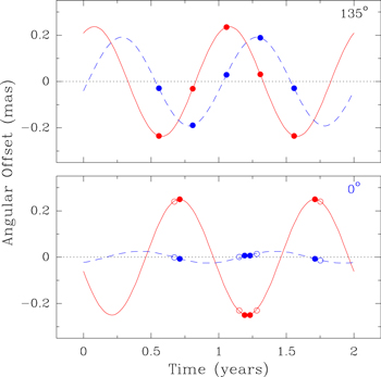
Figure 1. Parallax signatures for two sources at 4 kpc distance in the Galactic plane: (top panel) at 135° longitude and (bottom panel) at 0° longitude. The red solid lines trace the East–West offsets and the blue dashed lines trace the North–South offsets vs. time of year. The plotted points indicate near-optimal sampling. See the text for details.
Download figure:
Standard image High-resolution imageWhen the parallax amplitude in the East–West direction is significantly larger than in the North–South direction, one should schedule observations near the extremes of the East–West parallax sinusoid. An optimal sampling of this sinusoid would be to place one observation at an extremum, followed by two observations six months later, and then a fourth one year later than the first. This scheme decorrelates all parameters in a parallax and proper motion solution. However, an undesirable aspect of using only four observations is that it leaves only one degree-of-freedom (after solving for offset, motion and parallax) with which to estimate realistic parameter uncertainties from post-fit residuals (see a detailed discussion in Reid et al. 2017). Better would be to use eight observations by doubling-up on each of the four described above, as indicated by the additional open circles in the lower plot of Figure 1.
The parallax sequences just discussed assume that the sources are detectable over a full year of observation. This is usually not an issue for methanol masers, but can be a problem for water masers. Assuming water masers come and go on a timescale of seven months, an optimized sequence starts at an East–West peak and includes six epochs at offset days of 0, 91, 155, 189, 241, 364 (or the reverse). This was determined by evaluating parallax accuracy for thousands of Monte Carlo simulations, in which the dates of observation were chosen randomly.
A single astrometric observing track should include three types of observations:
3.1. Fringe Finders
Fringe-finder (a.k.a. manual phase-calibrator) sources are strong, compact sources which are used to "find" interferometric fringes and establish clock offsets and drifts at each antenna for use in the correlator. These sources should have mas-accurate positions, so as to avoid residual delays changing significantly over an observing track, and, ideally, little source structure. After correlation, one (or more) of these scans are used to estimate and remove electronic delay and phase differences among separate intermediate frequency (IF) bands. Always have at least 2 different fringe-finders observed briefly (e.g., 1 minute on-source) every couple of hours.
3.2. Geodetic Blocks
Geodetic blocks typically consist of rapid observations of a dozen calibrators spread across the sky and observed over a large range of source zenith angles (θZA). The goal is to measure broadband (group) delays and fit for clock and residual atmospheric path-delays to cm-level precision (Reid et al. 2009). For a given signal-to-noise ratio, group-delay precision scales inversely with spanned bandwidth. Thus, one should maximize the spanned bandwidth for best precision, even if this involves gaps in the frequency coverage. Since fitting delay involves Fourier transforming frequency to delay, the frequency coverage should minimize delay sidelobes. For example, four IF bands, centered at relative frequencies of 0, 1, 4 and 6 ×Δf, yield a "minimum-redundancy" sampling of integer multiples of 1 through 6 Δf. All calibrators must have positions accurate to ≲1 mas, in order for measured residual delays to be dominated by atmospheric, not position, errors.
It is best to observe geodetic blocks at a high frequency (e.g., 24 GHz), so as to minimize the contribution of the dispersive delay from the ionosphere. For dispersive delays, the interferometer phase at frequency ν is shifted by

where c is the speed of light, re is the classical electron radius, and Ne is the electron column density along the line of sight. Note that the phase shift is negative. The phase delay, τp, is given by
and the group delay, τg, is given by
Note that the group delay has the opposite sign of the phase delay (and the radio signal phase shift) for a dispersive delay. Combining the phase shift and group delay formulae yields the relation

In other words, when correcting the interferometer phase for a change in ionospheric group delay, one must flip the sign of the correction compared to a change in tropospheric delay. With a mix of dispersive and non-dispersive delays, corrections for group delays can be combined, but phase-delays cannot.
If one observes geodetic blocks at frequencies below about 15 GHz, it is best to measure multi-band delays at two well-spaced frequencies in order to estimate and remove the dispersive component of the delay from the total delay, yielding pure non-dispersive delay for each source. Note that solving for a zenith delay-error with pure dispersive delays, and then using an ionospheric mapping function to predict delays along a ray-path to a source, does not seem to improve astrometric accuracy. For example, at the high altitude of the ionosphere, rays from a source at, say, a zenith angle of 45° will pass through the ionosphere ≈400 km from the antenna site, likely creating a significant azimuthal dependence. It may be possible to solve for and remove an azimuthal dependence, but this has not yet been demonstrated.
3.3. Phase-reference Blocks
Phase-reference blocks involve cycling between sources well within the interferometer coherence time, which is usually limited by short-term fluctuations in tropospheric water vapor and produce phase changes proportional to observing frequency. For reasonably dry sites, the time spanned between (the centers of the) phase-reference scans should be less than about 40 s at 43 GHz, 80 s at 22 GHz, and 260 s at 6.7 GHz. For example, if a calibrator (C) is the phase reference for a target (T), the sequence could be C, T, C, T, ... with scan durations of 40 s at 22 GHz. Note that scan durations include slew and settle times, so on-source (dwell) times will be less. For a strong target and weak calibrator, so-called inverse phase referencing can be used: T, C, T, C, ... . At frequencies well above 10 GHz, such sequences are adequate, and if more than one calibrator can be found within about 2° of the target, they can be used to give quasi-independent relative positions (provided the calibrators are well separated on the sky) and to provide a check on potential problems associated with jet-like structures in some calibrators.
At frequencies below ∼10 GHz, MultiView can yield excellent astrometric accuracy (Rioja et al. 2017). Ionospheric electron densities follow the Sun, and residual path-delays can be approximated by ionospheric "wedges" and modeled with linear gradients (a tilted plane) on the sky. Using calibrators which surround the target, an observing sequence with four calibrators could be as follows: C1, C2, T, C3, C4, T, .... This approach involves fitting the phases from the four calibrators nearest in time to the target for a given interferometer baseline to a tilted phase-plane:

where ϕT is the desired phase at the target position, Sx and Sy are phase-gradients in the x and y directions, and Δx and Δy are angular offsets from the target position.
In general, three calibrators are the minimum number needed to fit a tilted phase plane. In the example above, I mentioned using four calibrators, as this provides the opportunity to identify and remove a "bad" calibrator, possibly owing to large phases associated with complex source structures. Interestingly, however, only two calibrators can be used, provided they nicely straddle the target source, such that a line between them passes very close to the target.
For MultiView to succeed, the entire cycle of calibrators and target must be completed in well under the interferometer coherence time (e.g., the time it takes for phases to wander by 1 radian). For example, at 1.6 GHz, Rioja et al. (2017) successfully used a cycle time of 300 s. It is critical that the phases on each calibrator are dominated by propagation delays and not, for example, by position errors or source structure. So, calibrator positions must be known to a small fraction of the interferometer fringe spacing on the longest baseline. Note, the calibrator positions can be updated by measuring relative positions to one of the calibrators (or possibly the target), which has a well determined absolute position. Calibrator phases can "wrap" past ±180°, owing to position or baseline errors or large residual tropospheric or ionospheric delays in the correlation process, and these phase wraps must be accounted for when fitting the phase-plane.
If the target source is sufficiently strong to use as the interferometer phase reference, inverse MultiView has some advantages. An observing sequence can be as follows: T, C1, T, C2, T, C3, T, C4, ... , and only the time between the centers of the target (T) scans needs to be less than the interferometer coherence time. Also, phase-wrap problems are reduced, compared to standard MultiView, as atmospheric phase-shifts should largely cancel between the target and each calibrator. Hyland et al. (2022) demonstrate that calibrators separated by up to 7° from the target can yield excellent results at 8 GHz. Typically this allows for many useful calibrators.
4. Data Calibration
4.1. Geodetic Block Analysis
The first step in calibration is to estimate clock and residual tropospheric delays at each antenna. This can be done with the geodetic-block data. Start by correcting the data for updated Earth's orientation parameters, antenna locations, source positions, and feed rotation. Also, ionospheric delays (usually not applied during correlation) should be removed, based on total electron content models. Then, electronic delays and phase offsets among different IFs and feeds should be "aligned" using a "comb" of frequencies inserted during the observations or performing a "manual" phase-calibration using a fringe-finder source.
Next, multi-band delays for a source on a baseline involving antennas i and j, τi,j = τj − τi , are fitted with antenna dependent clock parameters and atmospheric zenith delay-errors, where each antenna's delay is given by

assuming other sources of delay error are small. The first two terms in Equation (3) correspond to a clock offset, T0, and a linear clock drift over time,  and ΔT is time relative to a reference time, best chosen near the center of the observations; the last term is the zenith (vertical) atmosphreric delay error scaled by the secant of the source zenith angle,
  , for the increased (slant) path-length through the troposphere.
1
Note, with interferometric data the clock parameters for one (reference) antenna must be held constant and usually are set to zero. However, since θZA varies differently for each VLBI antenna, one can solve for the zenith delay at all antennas. Geodetic blocks with a dozen calibrators can take about 30 minutes to complete, depending strongly on antenna slew speeds, and should be done every 2–3 hr in order to monitor and correct for changing conditions.
, for the increased (slant) path-length through the troposphere.
1
Note, with interferometric data the clock parameters for one (reference) antenna must be held constant and usually are set to zero. However, since θZA varies differently for each VLBI antenna, one can solve for the zenith delay at all antennas. Geodetic blocks with a dozen calibrators can take about 30 minutes to complete, depending strongly on antenna slew speeds, and should be done every 2–3 hr in order to monitor and correct for changing conditions.
An often overlooked aspect of differential astrometry is that the tropospheric delay difference between a target and a calibrator at a given antenna is given by
At large zenith angles, both  and
and  blow up. While this can be leveraged to increase geodetic block sensitivity, large θZA observations should be avoided for phase-referencing astrometry.
Examples of geodetic block data from two baselines of VLBA observations are shown in Figure 2. Data were taken near 3 and 7 GHz and the dispersive component of delay (owing to ionospheric electrons) was calculated and subtracted from each measurement, leaving pure non-disperive delays. The left panels plot multi-band (group) delays and the right panels show fringe rates. Green dots are the measurements, blue circles are the fitted model and red symbols are residuals. The upper plots (for the baseline with antennas 5 and 8) show good data; one can see a uniform clock drift of about +0.3 nsec hr−1 and most residuals are ≲0.1 nsec (or ≲3 cm of path delay). The lower plots (for the baseline with antennas 6 and 8) show a serious problem. There is a large clock-drift rate of −2.5 nsec hr−1 evident between 11 and 15 UT (corroborated by an average fringe rate of about −3 mHz, corresponding to  for observations at ν = 5 GHz). While this is not necessarily a problem, there is a large clock jump between the third and fourth geodetic blocks (i.e., somewhere between 15:05 and 16:15 UT). Note that the residuals, while not as small as for baseline 5–8, are reasonably close to zero. This can happen as spurious large zenith-delay parameters can partially compensate for mismodeling the clock as a linear drift. So, simply looking for small residuals is not sufficient to spot problems. Clearly the clock jump occurred at antenna 6 (since antenna 8 is common to both baselines and the jump does not show up in baseline 5–8). Therefore, data involving antenna 6 from 15:05 to the end should be flagged, both in the geodetic block and phase-referencing files, and the geodetic block data should be re-fitted.
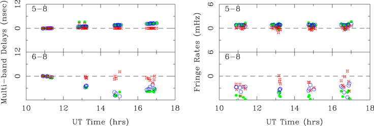
Figure 2. Geodetic block examples. Plotted are multi-band (group) delays (left panels) and residual fringe rates (right panels) vs. time. Measurements are green dots, best-fitting model values are blue circles, and "data minus model" residuals are red stars. The top row is for a well-behaved baseline, whereas the bottom row shows a serious problem—a clock jump between 15:05 and 16:15 UT.
Download figure:
Standard image High-resolution imageFinally, it is always a good idea to check that the clock and tropospheric delay corrections work well by applying them to the geodetic block data, re-fitting for multi-band delays, and verifying that the residual delays are ≲0.1 nsec. Alternatively, since many geodetic block sources are strong, after applying the corrections, one can simply plot phase versus frequency across all IFs and feeds and visually verify that the response is nearly flat.
4.2. Phase-referencing Block Analysis
The phase-referencing data require standard calibration steps, 2 with the addition of tropospheric delay calibration using the results of the geodetic-block fits, and for low-frequency observations substitution of MultiView for standard phase referencing. For example, calibration steps could be as follows:
- 1.Flag any bad data.
- 2.Convert interferometer visibilities (correlation coefficients) to Jansky units, using measured system temperatures and antenna gain curves, as well as any other known amplitude corrections (e.g., digitization loses).
- 3.Adjust delays and phases as done in the preliminary calibration of the geodetic block data (using updated Earth's orientation parameters, antenna locations and source positions, and applying ionospheric TEC models.).
- 4.Correct phases for antenna feed rotations; for example, for circularly polarized feeds shift phases by the feed parallactic angles with opposite signs for right and left circularly polarized feeds (and be sure to verify the proper sign convention). Note, this holds for linearly polarized feeds correlated against circularly polarized feeds, but for linear against linear feeds there is no phase shift induced by feed rotation. The conversion of VLBI data with some or all antennas having linearly polarized feeds to a common circularly polarized basis is complicated and deserves its own paper (see e.g., Martí-Vidal et al. 2016).
- 5.Apply clock and tropospheric delay corrections based on fitting geodetic block data. Then remove electronic delays and phases among IFs and feeds using either a calibration frequency comb (inserted at the receiver) or using a manual phase-calibration on a strong source. For spectral-line sources (e.g., masers) a subtle but serious problem can occur in this step. If a second-pass correlation is done which retains only a portion of the total IF bandwidth (so-called "zoom mode" used to limit the number of spectral channels when high spectral-resolution is desired), then one should also correlate the manual phase-calibration source(s) in the same manner and apply them to the spectral-line data. One cannot directly transfer the manual phase-calibration from broadband to narrowband data without considering the frequency location of the narrowband data relative to the edge frequency of its associated broadband, and some software analysis packages (i.e., AIPS and CASA) do not have this capability.
- 6.If the local oscillator was held constant during the observing track, then spectral-line sources will shift in frequency owing to the Earth's rotation and orbit about the Sun. Then interferometer visibilities should be corrected to hold a spectral line steady in frequency. If the visibilities are in the delay-lag domain, V(τ), this can be accomplished by an appropriate linear shift of visibility phase as a function of delay-lag, which corresponds to a shift in spectral frequency (by the Fourier transform shift theorem). If, instead, the visibilities are in the frequency domain, V(ν), one can Fourier transform to delay-lag, perform the linear phase shift, and then inverse Fourier transform back to frequency.
- 7.Phase reference the data. This can use a single source, either a calibrator (standard phase-referencing) or the target (inverse phase-referencing), or it can involve multiple calibrators (MultiView). Figure 3 shows three simulated examples of reference phases calculated from a single source. The top panel shows high SNR phases which might be obtained at ∼1 cm wavelength. The slow phase wander of hundreds of degrees of phase over hours is typical of path delays of ∼1 wavelength owing to variable water vapor. Within groups spanning about 15 minutes, the phases look "worm-like," which comes from small-scale fluctuations in water vapor, and one can reliably interpolate between individual points where the source to be referenced was observed.The middle panel of Figure 3 shows the same simulated data, except a low SNR of unity was used for each point. Interpolation between adjacent points would be very inaccurate and, when applied to another source, imaging would be considerably degraded. The bottom panel shows the effects of a large error in the position of the reference source, as evidenced by the "patterned" appearance made by rapid phase wrapping. Other errors, such as incorrect baselines or uncompensated clock drifts, can also do this. In this case, differential astrometric accuracy would be degraded by second-order effects of phase referencing as discussed earlier.As outlined in Section 3, at frequencies below ∼10 GHz, path-delays from ionospheric "wedges" can be removed from data with the MultiView calibration technique. Figure 4 shows simulated phases on one baseline at an instant in time for four calibrators surrounding a target. A tilted plane fitted to the calibrator phases as a function of (X,Y)-offset yields a phase of 50° at the position of the target source, which could then be removed from the target source data prior to astrometric measurements.As discussed in Section 3, phase wraps can be a serious problem. Figure 5 gives a simple example of a phase-wrap issue. The phase for the C3 calibrator, coming from the
 of an interferometer visibility, is generally defined between −180° and +180° and, in this example, is −175°. However, this phase should be +185° (i.e., −175° + 360°) and must be set to that value when fitting a MultiView tilted-plane to all calibrator phases. Otherwise, MultiView would return a spurious phase to the target.If the target source is sufficiently strong and compact so as to yield a high SNR in a single scan, it can be used as a "preliminary" phase reference for the surrounding calibrators (so-called inverse MultiView). This has the important advantage of pre-calibrating the data on a shorter timescale than standard MultiView, which requires cycling around all calibrators and the target well within the interferometer coherence-time limitation. This pre-calibration also results in "differenced phases," which can diminish phase-wrap problems. The next step in inverse MultiView is the same as standard MultiView, i.e., fitting a tilted plane to the differenced phases of the calibrators and subtracting the phase offset at the target position from the target phases (which were zero after the pre-calibration step). This returns "clean" phases, which give the desired position information for the target. Hyland et al. (2022) have demonstrated that inverse MultiView can work well for 8 GHz observations and achieve ≈20 μas (single-epoch) astrometry.It is essential that the calibrators used for MultiView have position errors small enough so as not to contribute significantly to the measured phases. If a priori positions are only known to, say, ±0.5θf
, then measured phases could have 180° unwanted contribution from their position errors. For a fringe spacing θf
∼ 1 mas, this corresponds to a position error of only 0.5 mas, and not all calibrators have this positional accuracy. However, what is more important is relative position accuracy among the MultiView calibrators. Relative position accuracy better than ±0.1θf
can usually be achieved through a first-pass of phase referencing and imaging of all sources relative to a single source with a very accurate position. After correcting the interferometer visibilities for the measured position offsets, one can then repeat the calibration sequence, now with greatly reduced contributions to phases from poor positions, and then do the MultiView step.
of an interferometer visibility, is generally defined between −180° and +180° and, in this example, is −175°. However, this phase should be +185° (i.e., −175° + 360°) and must be set to that value when fitting a MultiView tilted-plane to all calibrator phases. Otherwise, MultiView would return a spurious phase to the target.If the target source is sufficiently strong and compact so as to yield a high SNR in a single scan, it can be used as a "preliminary" phase reference for the surrounding calibrators (so-called inverse MultiView). This has the important advantage of pre-calibrating the data on a shorter timescale than standard MultiView, which requires cycling around all calibrators and the target well within the interferometer coherence-time limitation. This pre-calibration also results in "differenced phases," which can diminish phase-wrap problems. The next step in inverse MultiView is the same as standard MultiView, i.e., fitting a tilted plane to the differenced phases of the calibrators and subtracting the phase offset at the target position from the target phases (which were zero after the pre-calibration step). This returns "clean" phases, which give the desired position information for the target. Hyland et al. (2022) have demonstrated that inverse MultiView can work well for 8 GHz observations and achieve ≈20 μas (single-epoch) astrometry.It is essential that the calibrators used for MultiView have position errors small enough so as not to contribute significantly to the measured phases. If a priori positions are only known to, say, ±0.5θf
, then measured phases could have 180° unwanted contribution from their position errors. For a fringe spacing θf
∼ 1 mas, this corresponds to a position error of only 0.5 mas, and not all calibrators have this positional accuracy. However, what is more important is relative position accuracy among the MultiView calibrators. Relative position accuracy better than ±0.1θf
can usually be achieved through a first-pass of phase referencing and imaging of all sources relative to a single source with a very accurate position. After correcting the interferometer visibilities for the measured position offsets, one can then repeat the calibration sequence, now with greatly reduced contributions to phases from poor positions, and then do the MultiView step.

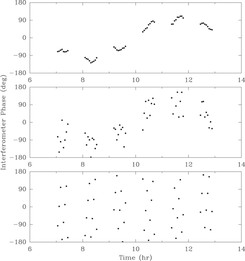
Figure 3. Interferometer reference phase simulations. Each dot represents a phase measured on a calibrator, to be interpolated between two adjacent (closely spaced) measurements and removed from the target source. A strong target can be used as the phase reference for a weak calibrator, so-called "inverse phase referencing," if desired. Top panel: high signal-to-noise phases showing small variations over ∼5 minutes and larger variations over hours. For high-quality differential astrometry, reference phases should resemble these. Middle panel: the same phases but generated with low signal-to-noise and these are far from optimal for phase referencing. Bottom panel: high signal-to-noise phases, but with a high residual fringe-rate as evidenced by rapid "phase wrapping." These indicate a large position error for the phase-reference source, or other geometric or clock errors, and are not suitable for accurate differential astrometry.
Download figure:
Standard image High-resolution image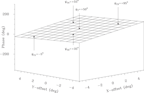
Figure 4. MultiView phase-calibration simulation of an ionospheric wedge with gradients of 10° and −5° of phase per degree of angular offset in the X- and Y-directions. Calibration sources are offset from the target at (X,Y) = (0°,0°) by (−4°, + 3°) for C1, (−2°, − 1°) for C2, (+3°, − 3°) for C3, and (+2°, + 3°) for C4. Fitting a tilted plane to the phases of the four calibrators (ψC1, ψC2, ψC3, and ψC4) returns the 50° phase at the origin to be removed from the target source. In general, the minimum number of calibrators needed to define the phase plane is three, but it can be useful to use four to test for a "bad" calibrator (e.g., with source-structure phase). In cases where the line between two calibrators comes very close to the target source, one can use only two calibrators.
Download figure:
Standard image High-resolution image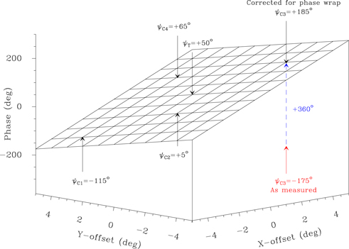
Figure 5. MultiView phase-calibration simulation, similar to that in Figure 4, but with larger gradients of 30° and −15° of phase per degree of angular offset in the X- and Y-directions. Fitting a tilted plane to the phases of the four calibrators (ψC1, ψC2, ψC3, and ψC4) would also yield the 50° phase at the origin to be removed from the target source. However, with the larger phase slope, the phase for C3 is now 185°, which would generally be reported as −175°. Fitting a tilted plane using that phase would result in a very large error in the slope and in the fitted phase at the target position. Such phase-wraps must be corrected for MultiView to work.
Download figure:
Standard image High-resolution image5. Things to Consider
A cardinal rule for astrometry used to estimate parallax and/or proper motion is to avoid changing any observational parameters over the entire program. This offers the best chance for canceling systematic errors. For example, if a source has structure within the resolution of the array and either the source or the interferometer (u,v)-coverage changes between observations, then one can get centroid shifts that are unrelated to parallax or proper motion and can degrade their measurement.
For sources with modest structure, such as a double with separation comparable to the interferometer resolution, accurate astrometry can usually benefit from some degree of "super-resolution." Often when imaging, one can use a round CLEAN restoring beam even if the dirty beam FWHM is elliptical. I have found it useful to separate compact emission components by setting the CLEAN restoring beam to
where the θmaj and θmin are the "dirty" beam's major and minor FWHM sizes, and using a moderate super-resolution factor, Sr , between 0.5 and 1.0.
While one can consider directly fitting interferometer phases for position offsets, it seems advisable to always make images in order to assess whether or not a source has a complicated structure. If a source (either the target, which might be an X-ray binary, or a quasar calibrator) has a jet-like structure, which changes among observing epochs, one should consider rotating the measured positions and the parallax/proper motion model to be along and perpendicular to the jet direction (e.g., see Miller-Jones et al. 2021). This allows one to down-weight the "corrupted" data in the jet direction and rely more on the "clean" data in the perpendicular direction.
When measuring group delays, e.g., for geodetic block observations, one should spread the spanned bandwidth in order to get more accurate delays. On the flip side, for phase-reference blocks, it is better to pack the bands together in order to minimize the frequency spanned and have less sensitivity to delay errors. Note that modern digital base-band converters (DBBCs) may introduce delay jumps when changing between different setups, and this can significantly degrade (or destroy) astrometry. If one's DBBCs have such problems, it might be best to observe geodetic and phase-reference blocks with the same electronic setup.
Calibrators offset from a target in decl. are often not as good for astrometry as those offset in R.A., since phases associated with atmospheric (zenith-angle dependent) delay errors can more closely mimic decl. than R.A. offsets.
6. Closing Thoughts
The most accurate parallax measurements to date have uncertainties near ±5 μas (see Table 1 of Reid et al. 2019, and references therein). In many cases, these come from measurements at 22 GHz and are limited by uncompensated tropospheric delays. Since these are likely to be quasi-random, parallax measurement can be improved with a greater number of observations (N), with precision scaling as 1/N1/2 (if optimally sampled). Currently, it is not clear if the non-dispersive phase-delays associated with fluctuations in water vapor are uncorrelated over several degrees on the sky or, instead, have a "planar" structure which could be addressed by MultiView calibration.
Three-dimensional (3D) kinematic distances offer a promising method of estimating distances to sources well past the Galactic center, where observed motions can approach 470 km s−1, i.e., twice the rotation speed of the Galaxy (Reid 2022). Thus, even at a distance of 20 kpc, this leads to a proper motion of about 5 mas yr−1, or over one year about 100 times the magnitude of the parallax amplitude. For young stars hosting masers, non-circular motions are ∼10 km s−1, and hence contribute less than a couple of percent to the distance error budget. Usually, proper motion can be measured much more easily than parallax, in part because motion precision scales as 1/N3/2 (for uniform sampling in time). Note, that if one observes a source at integer year intervals, the parallax effect vanishes, simplifying the motion measurement. Measurements with future VLBI arrays, including the SKA and the ngVLA, may be able to obtain hundreds-to-thousands of 3D kinematic distances for very distant Galactic sources.
Footnotes
- 1
While
is appropriate for a plane-parallel atmosphere and is a reasonable approximation for slant path delay, better θZA "mapping functions" which account for the Earth's curvature and finite atmospheric thickness are a significant improvement for observations at large zenith angles; see Thompson et al. (2017). - 2
see http://www.aips.nrao.edu/vlbarun.shtml for examples.
