The SNAD Viewer: Everything You Want to Know about Your Favorite ZTF Object

Modern astronomical surveys have drastically changed the process of astronomical data analysis. Traditionally, the field of astronomy was based on small data sets. Each of them gathered, analyzed, and reported by small research groups. Recently, the situation has drastically transformed into big data volumes, involving a large number of individuals at each stage of the process: from data ingestion to the final publication of scientific results. This long-predicted new paradigm (e.g., Szalay & Gray 2001) fostered the development of crafted infrastructure within each survey, including strategies for storage, indexing, and archiving protocols specifically designed to fulfill the needs of a given scientific goal or community. The resulting data environments have enabled the successful application of machine learning techniques in astronomical data, especially for classification and regression tasks—two of the most well-known examples being photometric classification of supernovae (e.g., Jones et al. 2018; Vincenzi et al. 2022) and photometric redshift estimation (e.g., Zhou et al. 2021; Abbott et al. 2022). For such supervised learning tasks, once the experiment design and analysis pipeline is finalized, researchers can rerun the entire machinery within the same survey, updating results as more data become available, in principle, without any need for visual screening of the original data.

At the same time, the observational nature of astronomy, coupled with the predetermined scanning strategies of large surveys, results in a tremendous potential for discovery (see, e.g., LSST-related reviews LSST Science Collaboration et al. 2009; Hambleton et al. 2022). In this context, human intervention is unavoidable. So far, even the most efficient machine learning algorithm cannot take into account all available data about each object it considers and can only provide good candidates as its output. These candidates usually need to be scrutinized by an expert who will put each of them in context and give meaning to a new discovery (Dick 2013). The expert, in turn, requires as much information as possible to form a comprehensive view of the new candidate and ensure its significance, as well as its novelty, reaching a final human conclusion. This means, for example, the researcher must gather data about the same object from multiple sources, build correlations between various wavelengths, and search for similar matches among well-known objects. In the specific case of transients or variables, one will also be interested in all available legacy data that can provide clues about their time evolution.

From the infrastructural point of view, this imposes a new set of requirements, which includes enabling easy visualization and cross-match between databases from different surveys, as well as with modern static catalogs, historical data, and derived data products. The SNAD team ¹² met this challenge when our experts aimed to analyze a large set of variable objects. That is the reason why The SNAD Zwicky Transient Facility (ZTF) viewer was originally built (hereafter, the Viewer): the Viewer was designed and built to optimize the allocation of human resources in astronomical investigative tasks. It helps experts make decisions about the class and properties of a given object faster, consolidating photometry, cross-matching, and other information about astronomical sources retrieved from multiple data sets and data archives, on a single web page. Moreover, the Viewer is publicly openly available online at https://ztf.snad.space.

The time spent by an expert trying to mine information about an object became crucial when we started using active anomaly detection algorithms (Ishida et al. 2021). These human-in-the-loop learning strategies use feedback from a domain expert to guide adaptations of hyperparameters of a traditional machine learning model, thus constructing a model tailored to the expert's own anomaly definition. The issue of scarce human resources for manual screening was already a limiting factor in the first stages of the SNAD pipeline development when we were dealing with a few thousand objects from the Open Supernova Catalog (Pruzhinskaya et al. 2019). However, it became unmanageable when faced with the Zwicky Transient Facility data releases ¹³ (ZTF DR).

The ZTF is a time-domain photometric survey currently in progress using the Palomar 48 inch Schmidt telescope (Bellm et al. 2019a, 2019b). It represents the state of the art of large-scale astronomical surveys and is considered a precursor to the upcoming Vera C. Rubin Observatory Legacy Survey of Space and Time ¹⁴ (LSST). For instance, data release 13, contains 4.37 billion light curves constructed from hundreds of billions of single-exposure extractions (see footnote 13).

There are a few publicly available tools that enable different levels of interaction with ZTF data, chief among them being the portals from ZTF community brokers (Section 2), IRSA IPAC, ¹⁵ and Fritz Astronomy Marshal. ¹⁶ Although they share some common features with the Viewer, broker systems were designed to deal with the data from the alert stream and to enable live analysis, while our goal was to explore the ZTF DRs. IRSA IPAC, on the other hand, provides a web user interface to access photometric data of surveys conducted by many different missions. Despite providing a convenient framework to handle ZTF DRs, its scope was not broad enough to fulfill the requirements of the SNAD anomaly detection pipeline. For expert analysis we required a portal providing instant access not only to a single object's light curve, but also to as much relevant contextual information as possible, including nearby ZTF DR objects and cross-matched results from different catalogs. Moreover, IRSA IPAC gives access to the most recent data releases, while for the SNAD team, it was crucial to support a set of legacy data releases, whose data might be involved in ongoing projects. Fritz Astronomy Marshal is a ZTF platform produced by the project's team and combining data from data releases, alert stream and cross-matching information from many catalogs. Access to the portal is restricted, but its source code is open and easy to run. However there is no easy way to ingest data-release photometry into the self-hosted instance of the system. Among non-ZTF frameworks with similar goals and infrastructure, we highlight the Open Supernova Catalog (OSC, Guillochon et al. 2017), the OGLE survey portal ¹⁷ (Udalski 2003; Udalski et al. 2015), and the ASAS-SN portal ¹⁸ (Kochanek et al. 2017; Jayasinghe et al. 2019), all of which are also integrated into our Viewer.

So far, the Viewer enabled all the ZTF-based results reported by the SNAD team (Malanchev et al. 2021; Aleo et al. 2022; Pruzhinskaya et al. 2022), whose summary can be found in the SNAD catalog, ¹⁹ currently hosting 144 candidate transients found by the SNAD team on ZTF DRs, while being absent from systematic searches from other groups.

Once it was made publicly available, the Viewer made its way from being an infrastructure project used exclusively by SNAD experts to becoming a valuable community resource for scrutinizing ZTF DR objects. It is currently being integrated into two ZTF brokers, ANTARES, ²⁰ (Matheson et al. 2021), and Fink ²¹ (Möller et al. 2021) and also in the Young Supernova Experiment marshal (Jones et al. 2021; Coulter et al. 2022). It also counts on average, a few dozen unique visitors per day from multiple countries. Beyond ZTF DRs, it provides access to the ZTF alert photometry and light curves from Pan-STARRS (Flewelling et al. 2020) and Gaia (Gaia Collaboration et al. 2016, 2022) surveys. It is an ideal entry point for the photometric investigation of various types of variable objects, including active galactic nuclei (AGNs), Milky Way variable stars, and microlensing events.

In what follows, we give details on the currently available services and their underlying implementation. Details about ZTF DRs are given in Section 2. Section 3 notifies users about the displayed information available and the choices which lead to them. Section 4 describes the only part of the Viewer that is, for the moment, private, where SNAD experts can annotate individual objects for subsequent internal use. Sections 5 and 6 describe details of our implementation and is directed toward developers and researchers who may find our experience useful in the construction of similar systems. We present our conclusions and plans for further developments in Section 7.

ZTF observes all of the visible Northern sky, covering from 25,000 to 30,000 square degrees having a field of view of 47 square degrees in gri passbands, and reaching a limiting median r-magnitude of ∼20.6 for a typical exposure of 30 seconds. It runs both public and private surveys with different cadence, exposure, and passband usage. The public survey is the source of the photometric alerts sent to community brokers, including ALeRCE ²² (Förster et al. 2021), AMPEL ²³ (Nordin et al. 2019), ANTARES (see footnote 21) (Matheson et al. 2021), Fink (see footnote 22) (Möller et al. 2021), Lasair ²⁴ and MARS. ²⁵ It operates using a differential photometry pipeline that triggers alerts using current observations and the ZTF reference catalogs. The survey has had two phases so far. During Phase I (2018 March–2020 September) it had a 3 days cadence for extra-galactic fields and a 1 day cadence for Galactic fields, while in Phase II (from 2020 December onwards) it switched to a homogeneous 2 days cadence all over the observable sky.

The public survey, which is openly available, uses 30 s exposures and primarily operates in gr passbands. The private survey used 60% of its observational time during Phase I and 50% during Phase II. It includes a significantly higher fraction of i-passband observations and also high-cadence data reaching hundreds of consecutive observations of the same field during a single night.

ZTF DRs were announced every six months from DR 1 (2019 May) to DR 4 and then the releases switched to a bimonthly schedule. Each DR covers observations for both private (from the start of the survey up to 18 months before the release date due to a proprietary period) and public surveys (from the start of the survey up to a few weeks before the release date). The ZTF DR photometric pipeline is different from the alert pipeline—it is based on source extraction for individual frames and subsequent cross-matching of these sources along all frames within a single pair of observation field/CCD quadrant and passband. This leads to two peculiarities of the data-release objects compared to the alert stream: (1) object light curves do not include non-detections, ²⁶ (2) a single sky source can be represented by more than a dozen ZTF DR objects due to three passbands and overlapping observation fields.

There are other important differences between the DRs and the alert stream: for example, source identifiers are independent and have different formats, the data-release pipeline does not contain the bogus-to-real image classification step which is a part of the alert production process (Duev et al. 2019), DRs provide Heliocentric MJD (HMJD) time of the middle of exposure while alerts use exposure start JD, among others. Alerts, in turn, are based on source detection via difference imaging, which is more effective for extragalactic sources. For example, most of the ZTF Bright Transient Survey supernovae (Fremling et al. 2020; Perley et al. 2020) are missing from the DRs. However, some robust SN candidates not presented in the alert stream were found in ZTF DRs by the SNAD team in Aleo et al. (2022), Pruzhinskaya et al. (2022). Moreover, the DR light curves have better limiting magnitudes and may also include observations that do not pass the difference imaging pipeline detection threshold (see Section 3.4.2 and Figure 4). To address these issues IPAC provides a service for PSF-fit forced-photometry, ²⁷ which has both deeper limiting magnitudes and includes non-detections, but can only be used for individual sky positions.

IRSA IPAC (see footnote 16) provides different ways to access ZTF DRs: through the web interface, light-curve API calls, and via bulk-downloadable files. Since the first two options are not scalable to access the dozens of millions of light curves needed for the SNAD anomaly detection pipelines, we decided to use bulk-downloadable files, which we converted to our internal database format (further described in Section 5.1). However, this option does not provide as much data as the other two interfaces, limiting object properties to: average coordinates, field, readout-channel identifiers, and passband. Similarly, detection properties are restricted to Heliocentric MJD of the middle of the exposure, the magnitude and its uncertainty, the color correction coefficient, and the quality flags.

It is difficult to overstate the importance of ZTF DR for time-domain astronomy. It has already motivated searches and studies of AGNs (e.g., Sánchez-Sáez et al. 2021), strongly lensed QSOs (e.g., Stern et al. 2021), microlensing (e.g., Rodriguez et al. 2022), variable stars (e.g., Chen et al. 2020; Kupfer et al. 2021), young stellar objects (e.g., Kuhn et al. 2021), eclipsing binary systems (e.g., Kosakowski et al. 2022) and, unexpectedly, supernova-like transients (Pruzhinskaya et al. 2022). Moreover, their volume and complexity, combined with their timely existence as a precursor to LSST, makes ZTF DR a unique ground for preparing data mining and machine learning techniques (Malanchev et al. 2021; Aleo et al. 2022) which will be of paramount importance for the next generation of telescopes and surveys. We did our best to make the Viewer a convenient place to inspect photometric and complementary ZTF DR data, a web portal that can serve all researchers interested in deep investigation of individual objects.

3.1. Homepage

The Viewer homepage, shown in Figure 1, gives a brief description of the website and references to the data sources available through the portal. Its header contains a login link (see Section 4 for SNAD internal resources description) and two search fields: one for ZTF object identifier (OID) and another one for cone search. The OID search field supports 15–16 digit strings for the ZTF DR identifier and 3-digit strings for the SNAD catalog objects (see footnote 20). The cone search field accepts an equatorial coordinate string in various formats ²⁸ as well as object identifiers which are resolved to sky positions using SIMBAD (Wenger et al. 2000). The cone search radius is to be specified in arcsecond—the default value is 1'' and the maximum supported radius currently is 60''.

Zoom In Zoom Out Reset image size

3.2. Cone-search Results Page

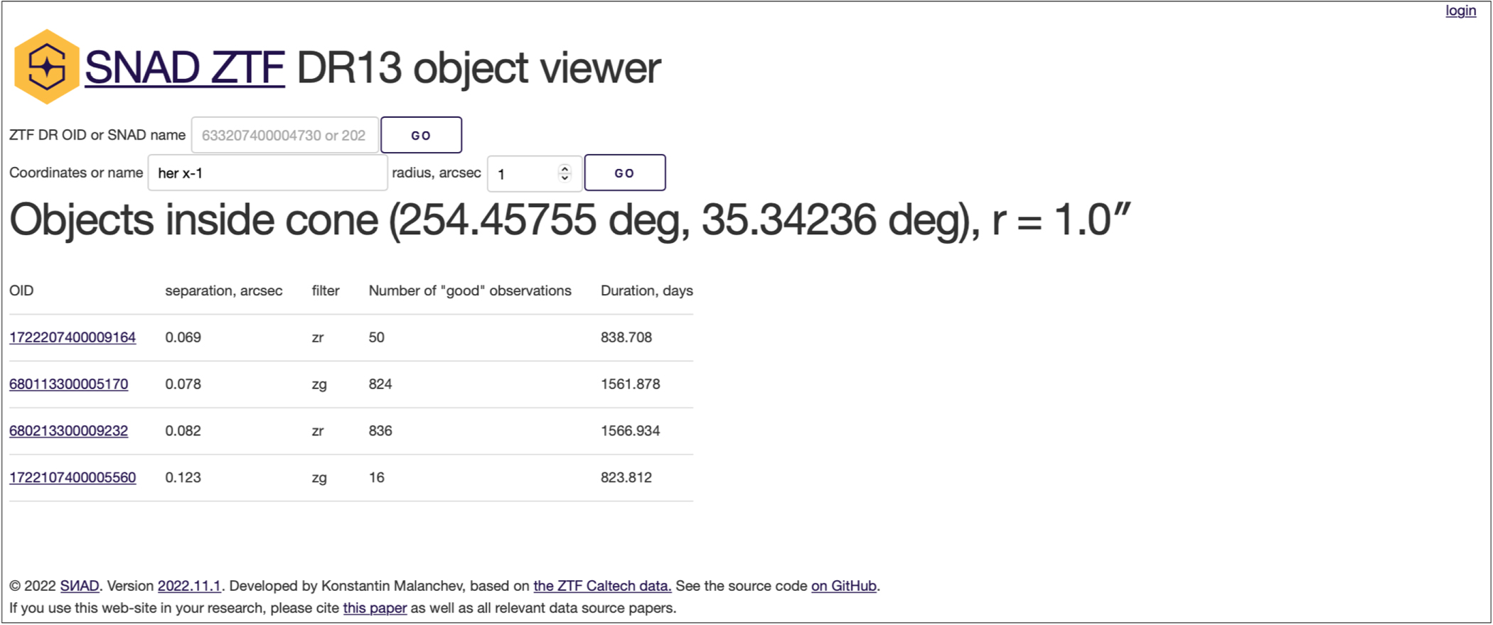
After the user requests a cone search, they are redirected to a page displaying the table of search results. This page has three states: (1) requested string cannot be parsed or resolved via SIMBAD, (2) no results are found, or (3) the search is successful and a table of matches is shown. For the last case, resolved coordinates of the sky position are shown as well as all matched ZTF OIDs. An example is shown in Figure 2. We note that no crossmatch to ZTF objects is performed at this step. Thus, due to the ZTF DR object definition, the user may see multiple object identifiers corresponding to a single sky source. After selecting one of the results, the user is redirected to the object page.

Zoom In Zoom Out Reset image size

3.3. ZTF Object Page

Figure 3 shows the upper part of the object page, the lower part contains external (non-ZTF) catalog cross-matches (see Section 3.6), light-curve features (see Section 3.7) and the ZTF DR photometry table. The ZTF object page is built from multiple blocks, and we describe the most important ones in the next sections.

Zoom In Zoom Out Reset image size

3.4. Light-curve Plot

The light-curve plot is the main element of the object page. By default, it shows ZTF DR light curves for the given object and all neighboring objects found within the cone of the default search radius (1''). Data points from the target object have larger markers, so that it is easier to distinguish them visually from those of nearby objects. This representation is configurable, and the user can hide light curves of arbitrary objects and change the search radius. It is also possible to display a "short" light curve, restricted to dates corresponding to those of the available private survey. This allows visualization of a homogeneous cadence and overall survey properties presented in ZTF observations. The SNAD team used this functionality in Malanchev et al. (2021), Pruzhinskaya et al. (2022), and Aleo et al. (2022).

A period-folded representation of light curves is also available, see an example in Figure 6. By default, it uses a period corresponding to the highest Lomb–Scargle periodogram peak (Lomb 1976; Scargle 1982) calculated for the target ZTF DR object (Section 3.7) and zero phase with respect to HMJD = 58000. The user can change both phase and period, which can possibly be obtained from multiple sources listed in the "Summary" section just below the plot (see Section 3.8).

Both the original and the period-folded light curves can be downloaded in PNG or PDF formats, generated using the matplotlib library (Hunter 2007). These plots display the ZTF object neighbors and the ZTF range and can also handle user-configured parameters such as custom titles and additional photometric data.

Another available customization for the representation of photometric data is the choice between magnitude and flux and between their apparent and difference values. Since ZTF DRs provide the photometric data in magnitudes, we transformed them into fluxes using the AB-system zero-point,

$$\begin{eqnarray}&&f={10}^{-0.4(m-8.9)}\,\mathrm{Jy},\end{eqnarray} \tag{ 1 }$$

$$\begin{eqnarray}&&{\sigma }_{f}=0.4\mathrm{ln}(10)\cdot f\cdot {\sigma }_{m},\end{eqnarray} \tag{ 2 }$$

where m and σ_m are the apparent magnitude and its uncertainty as reported in the ZTF DR, f and σ_f is our estimate of the apparent spectral flux density and its uncertainty in janskies. The ZTF reference catalog (see Section 6.4 for the technical details) provides the reference magnitude and corresponding uncertainty for each OID. When a user selects the differential photometry option, we load these values for each object and use them for differential flux density estimation,

$$\begin{eqnarray}&&{\rm{\Delta }}f=f-{f}_{\mathrm{ref}},\end{eqnarray} \tag{ 3 }$$

$$\begin{eqnarray}&&{\sigma }_{{\rm{\Delta }}f}=\sqrt{{\sigma }_{f}^{2}+{\sigma }_{{f}_{\mathrm{ref}}}^{2}},\end{eqnarray} \tag{ 4 }$$

where f_ref and ${\sigma }_{{f}_{\mathrm{ref}}}$ are the reference flux density and its uncertainty determined by Equations (1) and (2). Difference magnitudes are considered to have asymmetric uncertainties,

$$\begin{eqnarray}&&{\rm{\Delta }}m=8.9-2.5\mathrm{lg}{\rm{\Delta }}f,\end{eqnarray} \tag{ 5 }$$

$$\begin{eqnarray}&&{\sigma }_{{\rm{\Delta }}m}^{+}=-2.5\mathrm{lg}\left(1-\displaystyle \frac{{\sigma }_{{\rm{\Delta }}f}}{{\rm{\Delta }}f}\right),\end{eqnarray} \tag{ 6 }$$

$$\begin{eqnarray}&&{\sigma }_{{\rm{\Delta }}m}^{-}=-2.5\mathrm{lg}\left(1+\displaystyle \frac{{\sigma }_{{\rm{\Delta }}f}}{{\rm{\Delta }}f}\right).\end{eqnarray} \tag{ 7 }$$

The user can change the reference values, which can be useful for cases where the ZTF reference catalog gives unsuitable reference magnitudes, e.g., when a reference image contains the considered object around its maximum light. An example of a difference flux density plot is shown in Figure 4.

Zoom In Zoom Out Reset image size

3.4.1. External Light Curves

Currently, three external photometry data sources are supported: the ANTARES (see footnote 21) broker for ZTF alert data, Pan-STARRS DR2 ²⁹ and Gaia DR3. ³⁰ The light-curve plot can include additional epochs from all of them. We used the corresponding APIs to perform a 5'' cone search centered on the ZTF object position and choose the closest object to be included in the Viewer light curve.

3.4.2. ZTF Alert Light Curve

Apart from the availability of non-detections, ZTF alert pipeline is intrinsically different from those in the DR (see Section 2 and Bellm et al. 2019b for details). Moreover, the alert stream delivered to the ZTF brokers may contain more recent observations. Therefore showing this data together with the ZTF DR light curves might bring important insights on the astronomical objects inspected with the Viewer. Moreover, ZTF alert users can find the ZTF DR useful to distinguish, for instance, a supernova from an AGN or a cataclysmic variable, which could have similar alert light curves, but different DR light curves (see Figure 4 for a real-life example of such a case). For this purpose we use the ANTARES (see footnote 21) broker (Matheson et al. 2021) API. ³¹

3.4.3. Pan-STARRS DR2

The Viewer also uses data from Pan-STARRS. ZTF uses photometric filters with passbands close to the Pan-STARRS filters, and also uses its data for photometric calibration. Moreover, both surveys operate in the northern hemisphere and cover roughly the same part of the sky. Finally, Pan-STARRS DR2 includes time-resolved photometry data in grizy passbands from a period before the start of ZTF: from 2010 to 2014 (Flewelling et al. 2020). All these make Pan-STARRS DR2 light curves complementary to ZTF data. Therefore we provide Pan-STARRS DR2 PSF photometry, and we use the MAST API ³² for data access.

Pan-STARRS DR2 gives calibrated flux densities in janskies, which we convert into AB-magnitudes using the inverse of Equations (1) and (2),

$$\begin{eqnarray}&&m=8.9-2.5\mathrm{lg}f,\end{eqnarray} \tag{ 8 }$$

$$\begin{eqnarray}&&{\sigma }_{m}=\displaystyle \frac{2.5}{\mathrm{ln}10}\displaystyle \frac{{\sigma }_{f}}{f}.\end{eqnarray} \tag{ 9 }$$

Pan-STARRS provides observation times according to the international atomic time standard at the midpoint of each observation. We transformed this value to Heliocentric MJD in UTC. An example of a combined ZTF-Pan-STARRS light curve is shown in Figure 5.

Zoom In Zoom Out Reset image size

3.4.4. Gaia DR3

The third data release of Gaia contains epoch photometry in G, BP and RP passbands covering observations between 2014 July 25 and 2017 May 28 (Eyer et al. 2022; Gaia Collaboration et al. 2022). The Gaia DataLink service ³³ (Dowler et al. 2015; Gonzalez-Núñez et al. 2019) provides access to epoch instrument fluxes, ${{\mathfrak{f}}}_{\mathrm{Gaia}}$. We used instrumental zero-points, zp, and their uncertainties, σ_zp, to convert fluxes to AB-magnitudes (Riello et al. 2021),

$$\begin{eqnarray}&&m=\mathrm{zp}-2.5\mathrm{lg}({{\mathfrak{f}}}_{\mathrm{Gaia}}),\end{eqnarray} \tag{ 10 }$$

$$\begin{eqnarray}&&{\sigma }_{m}=\sqrt{{\left(\displaystyle \frac{2.5}{\mathrm{ln}10}\displaystyle \frac{{\sigma }_{{{\mathfrak{f}}}_{\mathrm{Gaia}}}}{{{\mathfrak{f}}}_{\mathrm{Gaia}}}\right)}^{2}+{\sigma }_{\mathrm{zp}}^{2}}.\end{eqnarray} \tag{ 11 }$$

Flux values and their uncertainties, in janskies, were then obtained using Equations (1) and (2).

Gaia uses the TCB time standard and provides the average transit Barycentric time. We converted it to UTC standard and assumed that for the purposes of the majority of the Viewer users, the few seconds-level difference between the Barycentric time and the Heliocentric time (e.g., Eastman et al. 2010) as given in ZTF DR, would not be considered significant. An example of a combined ZTF–Gaia light curve is shown in Figure 6.

Zoom In Zoom Out Reset image size

3.5. ZTF FITS

We added an embedded JS9 ³⁴ (Mandel & Vikhlinin 2022) FITS image widget to the right of the light-curve plot (see Figure 3). The user can click on any ZTF DR photometry point to load the scientific image corresponding to that observation. The image is centered on the object position, marked by a green dot, and the default zoom factor is equal to unity, which means that a single screen point corresponds to a single CCD pixel. While we used the JS9 widget without the toolbar and the menu, the link to the fully functional JS9 viewer is provided just below the image itself, in case the user requires additional functionalities.

We used the IRSA IPAC archive ³⁵ as the original source of these FITS images. Additionally, we employed our own proxy to work around the problem of loading data into the JS9 widget from a location not allowing cross-origin resource sharing (CORS) ³⁶ due to safety concerns (see Section 6.4 for our implementation details). The archive uses the following path encoding for scientific FITS images: YYYY/MMDD/MJDFRA/ztf_YYYYMMDDMJDFRA_FIELDN_PB_c CN_o_qQ_sciimg.fits, where YYYY, MM, DD are the year, month, and day of observation in UTC, MJDFRA is the fractional part of the MJD at the start of exposure, FIELDN is the ZTF field number, PB is the ZTF passband name (zg, zr or zi), CN is the CCD identifier (01 to 16), and Q is the CCD quadrant identifier (1 to 4). A typical example of a path for a source is: 2019/0314/432616/ztf_20190314432616_000633_zr_c 07_o_q4_sciimg.fits.

The main issue we faced while assembling this path is that the ZTF DR bulk-downloadable files (Section 2) do not provide enough information to allow for their unambiguous reconstruction. They provide only the HMJD and the read-out channel identifier rcid (0 to 63). The latter is sufficient to reconstruct the CCD and quadrant identifiers,

$$\begin{eqnarray}&&{\mathtt{CN}}=\unicode{x0230A}\displaystyle \frac{{\mathtt{rcid}}}{4}\unicode{x0230B}+1,\end{eqnarray} \tag{ 12 }$$

$$\begin{eqnarray}&&{\mathtt{Q}}={\mathtt{rcid}}\mathrm{mod}4+1.\end{eqnarray} \tag{ 13 }$$

The more challenging part is reconstructing the MJD of the beginning of the exposure from the HMJD in the middle of it, without information about the exposure duration and having a precision of around a second (HMJD is rounded to five decimals). We solved this issue by getting an estimate of the required MJDFRA ³⁷ and by identifying the closest available value in the archive, which resulted in a working approximation for the FITS file path.

3.6. External Catalogs Cross-matching

3.7. Light-curve Features

3.8. Summary Section

Beyond the public user-interface features described above, the Viewer has a private section called the Knowledge Database (KDB), which is filled and used by authorized experts of the SNAD team. The KDB was built to allow SNAD experts to share expertise among themselves. Whenever a given candidate is presented to an expert, it is followed by extensive analysis based on visual screening of all the photometric data in the Viewer, literature review, photometric model fitting, or follow-up observations. All this information is combined in a final judgment about the nature of the candidate, which is recorded by the expert in the KDB.

After login, the expert is directed to an enhanced version of the object page, which contains one more block representing the KDB record for the current OID (Figure 7). The block displays the most recent classification and the description record for the object, as well as a history of all previous records, including its date and author. The expert can also provide a description of the object in free text format, mainly used to clarify classification choices and extra data sources.

Zoom In Zoom Out Reset image size

The classification is represented in terms of a non-hierarchical tag system so that each object can have multiple tags. The tag itself is a short string that shows an associated description at pointer hover. Experts can change the order tags and add new ones by accessing the tag editor page. Since the SNAD team works as one coherent group of specialists, every user has the power to change the tag list, which is available to all users. However, the same structure can be personalized for other projects or collaborations, allowing each user to see their own set of chosen tags if necessary.

Currently, the KDB contains more than 50 tags which can be split into the following categories: types and sub-types of variability such as "Eclipsing," "EA," "EB," and "EW;" ⁴⁴ image and photometric pipeline artifacts like "artifact" and "defocusing;" properties of classification such as "uncertain" and "non-cataloged" which are only meaningful when combined with other tags; and cross-team communication tags like "TNS_candidate," which states the object is worth submitting to TNS. A detailed description of the currently available tags was reported by Pruzhinskaya et al. (2022).

Figure 8 shows the KDB table page with an interactive table of all tagged objects. An expert can apply filters to individual columns, for example, to see all objects marked with a specific tag or all records modified by someone. The KDB also has programmatic access, which can be used for more sophisticated analysis. We further describe the implementation details of the KDB API service in Section 6.5.

Zoom In Zoom Out Reset image size

In the context of the adaptive learning algorithms developed by the SNAD team, the final state of a specific learning model is a direct consequence of the feedback provided by the expert during training. Thus, the historical record stored in the KDB is crucial to allow for reproducibility of results, as well as to isolate probable causes for divergence in models trained by different experts. The historical record also allows experts to immediately access each other's judgments, which has proven efficient, especially when experts come from different scientific backgrounds or train models with different goals. Finally, the SNAD team is currently developing machine learning models which aim at using tags from the KDB as prior information. This will optimize the allocation of human resources since experts will not need to start from scratch when training a model for a new purpose.

The viewer infrastructure is built from multiple services which mainly communicate via the HTTP protocol (Fielding et al. 1999). We define in this paper a module as a program configured as a single Docker ⁴⁵ container, a service as a closely connected set of modules that are configured by a single Docker-Compose file, and a service instance as a set of containers, volumes, and networks deployed by a docker-compose tool. Since the Viewer does not have high availability requirements, most of our services have only one instance running on a virtual private server (VPS). However, the ZTF DR database API (see Section 6.2.1) and the ZTF FITS caching proxy (see Section 6.4) services have significant hardware requirements which do not meet our VPS budget. Therefore we have instances running those services at dedicated servers located at two academic institutions (currently at the Sternberg Astronomical Institute and at the University of California, Irvine). Individually, each of these dedicated servers has lower availability than the VPS due to possible network, power, and hardware issues. Nevertheless, we duplicated the services in those two services, increasing the availability at the system level.

The choice of the multi-service architecture behind the Viewer design is based not only on budget limits and availability requirements but also on the need for low maintainability effort and easy deployment. Most of the services are self-consistent and require no persistent data for deployment to a different host, which is a desirable feature whenever the host server needs to be replaced. This is also an advantage in case we decide to perform additional on-demand deployments in the future, dispatching cloud instances automatically for instance. Issue localization and debugging are also easier in a multi-service architecture because, generally, in the case of unexpected problems, a service will fast-fall, making it easy to identify which service is not available at a given moment. The same reasoning applies to our choice of having one database management system (DBMS) module per service instead of a single centralized DBMS service holding multiple databases: (1) with a single DBMS instance, any outage or network issue would cause an interruption of all services relying on it, and (2) additional network configuration would be required to help services discover and secure access to this DBMS instance, while, in our approach, Docker compose solves this problem via virtual networks connecting each API module to its DBMS companion. The Viewer service itself is not sensitive to the degradation of other services; for example, if one of our catalog services goes down, the Viewer shows that this catalog is not available, but otherwise, it continues to operate as usual. The multi-service approach also allows the use of individual services by multiple projects; for instance, the SNAD collaboration accesses the Viewer APIs via Python scripts and notebooks.

In our architecture, individual services are configured as a set of Docker containers bundled to have a common private virtual network and volumes using Docker Compose. Each of the servers we use has a common infrastructure configured as a dedicated Docker Compose and includes the following modules,

• 1.  
  nginx-proxy ⁴⁶ is a reverse proxy that gives access to our HTTP services via different domain names (virtual hosting);
• 2.  
  acme-companion ⁴⁷ gets and automatically renews TLS certificates via Let's Encrypt authority, ⁴⁸ making it possible to have secure HTTPS access throughout the system;
• 3.  
  dyndns53 ⁴⁹ creates and updates type A CNAME records for service domain names via Amazon Web Services' Route 53 DNS. ⁵⁰

The Viewer design choices are similar to those the ZTF project team made for their Fritz Asrtronomy Marshal (see footnote 17). Its infrastructure is also based on multi-service architecture, services are managed by Docker-Compose and communicate via HTTP RESTful APIs. The Fritz Marshal also acts as an alert broker via its Kowalski component. ⁵¹ Some of the software and framework choices of Fritz and the Viewer also match: both use Python as a main programming language and aiohttp ⁵² as a framework for APIs. However some design and software choices differ, for instance, Fritz uses a document data model via the MongoDB data management system, while the Viewer uses relational model (see Section 5.1). Both approaches have their pros and cons, and as we mention later, our data model choice was primary based on the requirements coming from the SNAD machine learning pipelines, while the document data model would work faster for the needs of the portal.

We show in Figure 9 the infrastructure of the Viewer, representing an overview of all the services and the individual modules. The data flow is represented using lines and arrows: the Viewer consumes data from many services and external APIs, while experts add records to the Knowledge Database using the Viewer. We further describe the implementation details of individual Viewer services in Sections 5.1 and 6.

Zoom In Zoom Out Reset image size

5.1. Data Storage for ZTF DRs

5.2. Development

As previously described, the Viewer is designed following a multi-service architecture. In this section, we present its most important services.

6.1. The Viewer Web-portal

6.2. Catalog APIs

6.3. Feature Extraction API

6.4. ZTF FITS Caching Proxy

6.5. Knowledge Database API

This work describes the SNAD Viewer which aims to help address one of the most daunting challenges of contemporary science: how to make sense of big data sets generated by modern experiments. In many fields with strong observational ties, like astronomy, despite undeniable progress in automatic learning techniques, a significant fraction of potential breakthroughs are still expected to require human screening and intervention for the foreseeable future. We conceived the SNAD Viewer to optimize the allocation of human resources in such tasks.

Our initial goal was to centralize external information about the objects present in ZTF data releases through a single web interface, thus allowing SNAD experts to provide feedback to adaptive learning pipelines more efficiently. However, we evolved the Viewer to be a host of our team expertise, and now it also hosts a knowledge database containing thousands of annotations which we expect to provide valuable priors to inform the training and design of future learning algorithms.

Our system is currently based on a multi-service infrastructure, which allowed us to achieve good development speed, simplicity, and the required level of availability. We built it using the Dash framework, giving our users a powerful interactive interface. It is currently highlighted at "Plotly and Dash 500" rating, ⁷⁵ and it is regularly used from all continents, but Antarctica, serving from a dozen to a few hundred unique visitors per day and responding to hundreds of thousands HTTP requests every month.

The SNAD Viewer framework has also proven to be resilient under different user conditions, and it is currently integrated into the ANTARES and Fink brokers, as well as into the Young Supernova Experiment marshal (Coulter et al. 2022). Moreover, it has enabled the development of all the SNAD projects using ZTF data (e.g., Malanchev et al. 2021; Aleo et al. 2022; Pruzhinskaya et al. 2022), including the discovery of lost transient candidates in ZTF DR (see footnote 20).

In this era of big data, the SNAD Viewer is an illustrative example of the potential enabled by the open science policies of 21st century astronomy. Its development was only possible due to the large efforts allocated to the maintenance of public data archives and APIs, which guarantees accessibility of final data products to the entire astronomical community, and consequently optimizes the scientific results from these data. It is also a statement on the effort necessary to nurture a truly interdisciplinary environment. The development of its features was, from the very beginning, guided by domain experts who voiced their needs and concerns raised during the analysis process. This experience will certainly be valuable once data from LSST becomes available.

Finally, the SNAD Viewer framework described in this work was designed to allow easy adaptation as well as scalability to other surveys. In the era of LSST, such data centralization about specific objects will be as important to most astrophysical domains as it already is today for multi-messenger astronomy. However to realize this vision, tools used for different science cases must be designed to be easily adaptable to the requirements of different research sub-fields. With the SNAD Viewer we present an example of such a tool, and its successful experience so far also demonstrates the great potential they hold for the future of astronomical discovery.

Authors are grateful to Kirill Sokolovsky, Adam Scott, Julien Peloton, and Vadim Krushinsky for the helpful discussions. We thank all users of the Viewer for their feedback and bug reports. We thank Clara Heinrich for her work in the illustration of Figure 9.

This research has made use of the NASA/IPAC Infrared Science Archive, which is funded by the National Aeronautics and Space Administration and operated by the California Institute of Technology. This research has made use of the SIMBAD database, VizieR catalog, and "Aladin sky atlas" access tool, operated at CDS, Strasbourg, France. This work has made use of results from the ESA space mission Gaia, the data from which were processed by the Gaia Data Processing and Analysis Consortium (DPAC). Funding for the DPAC has been provided by national institutions, in particular the institutions participating in the Gaia Multilateral Agreement. Some of the authors are members of the Gaia Data Processing and Analysis Consortium (DPAC).

We used the equipment funded by the Lomonosov Moscow State University Program of Development. This work made use of server hosting services from the Donald Bren school of Information and Computer Sciences of the University of California, Irvine, and of a machine acquired with the UCI 2021-2022 Professional Development Award. This work made use of the Illinois Campus Cluster, a computing resource that is operated by the Illinois Campus Cluster Program (ICCP) in conjunction with the National Center for Supercomputing Applications (NCSA) and which is supported by funds from the University of Illinois at Urbana-Champaign.

The reported study was funded by RFBR according to the research project 20-02-00779. M.V.P. acknowledges the support by the Interdisciplinary Scientific and Educational School of Moscow University "Fundamental and Applied Space Research" E.E.O.I. and E.R. received financial support from CNRS International Emerging Actions under the project Real-time analysis of astronomical data for the Legacy Survey of Space and Time during 2021-2022. P.D.A. is supported by the Illinois Survey Science Graduate Fellowship from the Center for AstroPhysical Surveys (CAPS) ⁷⁶ at the National Center for Supercomputing Applications (NCSA). A.K.M. acknowledges the support from the Portuguese Fundação para a Ciência e a Tecnologia (FCT) through grants UID/FIS/00099/2019 for CENTRA and EXPL/FIS-AST/1368/2021. Supported by Nonprofit Foundation for the Development of Science and Education "Intellect."