Abstract
The Full-disk vectorMagnetoGraph (FMG) instrument will carry out polarization observations at one wavelength position of the Fe I 5324.179 °A spectral line. This paper describes how to choose this single wavelength position, the relevant data-processing and the magnetic field calibrations based on the measured polarization signals at one single wavelength position. It is found that solar radial Doppler velocity, which can cause the spectral line to shift, is a disadvantageous factor for the linear calibration at one wavelength position. Observations at two symmetric wavelength positionsmay significantly reduce the wavelength shift effect (∼ 75%), but simulations show that such polarization signals located at the solar limbs (e.g., beyond the longitude range of ±30°) are not free from the effect completely. In future work, we plan to apply machine learning techniques to calibrate vector magnetic fields, or employ full Stokes parameter profile inversion techniques to obtain accurate vector magnetic fields, in order to complement the linear calibration at the single wavelength position.
Export citation and abstract BibTeX RIS
1. Introduction
The Full-disk vector MagnetoGraph (FMG, Deng et al. 2019) instrument is one payload on the Advanced Spacebased Solar Observatory (ASO-S, Gan et al. 2019) that will be launched in early 2022. It aims to unravel the build up of magnetic energy and its release during flares and coronal mass ejections (CMEs), to obtain a profound understanding of the role of the magnetic field in solar eruptions. In addition, the instrument will detect and monitor the magnetic field evolutions of sunspots, active regions and complexes of active regions in real time, and will accordingly estimate the probability of flare occurrence so as to facilitate forecasting space weather. Based on the above considerations, the FMG is designed to measure full-disk solar vector magnetic fields at a high cadence of 2min. For routine observations, Stokes Q, U and V will be taken at one wavelength position (e.g., −0.08 Å) of the Fe I 5324.179 Å absorption line. After calibrations, the magnetic sensitivities are expected to attain levels of 15 and 270 G for longitudinal and transverse components of the vector magnetic fields, respectively.
The data from FMG are divided into four levels, from Level 0 to Level 1 and Level 2, as well as Level Q (designed for a quick look). This paper will only focus on how to reduce the first three levels' data. Level 0 data are those directly downloaded from ASO-S including Stokes Q, U and V maps, telemetry information, calibration data and header keywords. They become Level 1 data once they undergo the processing of subtracting the dark field, dividing by the flat field, calibrating the working line, correcting for Stokes I-to-Q, −U and −V, and for Stokes V-to-Q and −U crosstalks, and calibrating into magnetic fields. Finally, Level 2 data are obtained by disentangling 180° ambiguity and removing projection effects.
Properties of the Fe I 5324.179 Å line and selection of the single filter position are introduced in Section 2. We present details of the processing of Level 1 data in Section 3. Removals of 180° ambiguity and projection effects are described in Section 4. Finally, we conclude in Section 5.
2. determination of the Single Wavelength Position
2.1. Properties of the Spectral Line
This spectral line is produced by the electron transition between the atomic energy levels  at 25899.989 cm−1 and e5
D4 at 44677.006 cm−1. The oscillator strength of the transition is fik = 0.1 and log(gifik) = −0.103 (Bard et al. 1991) or fik = 0.087 and log(gifik) = −0.24 (Nave et al. 1994), where gi = 9 is the degeneracy of the low level involved in the transition. The line exhibits normal moderate Zeeman splitting with an effective Landé factor geff = 1.5. It is found that the effect of Faraday rotation is less significant in the observations taken near the line center of Fe I 5324.179 Å than those taken near the line center of Fe I 5250.22 Å that is used by the Video Vector Magnetograph at Marshall Space Flight Center (West & Hagyard 1983; Hagyard et al. 2000; Su & Zhang 2004; Su et al. 2006; Zhang 2019). As with a low level excitation potential of Ei = 3.197 eV, it is less sensitive to temperature variation than the Fe I 5250.22 Å (Ei = 0.12 eV) and Fe I 6173.32 Å (Ei = 2.2 eV) lines. The Fe I 6173.32 Å line is the working spectral line of the Helioseismic and Magnetic Imager (HMI) onboard the Solar Dynamics Observatory (SDO; Schou et al. 2012b). Therefore, calibration coefficients for the Stokes Q, U and V parameters measured with the Fe I 5324.179 Å line in the quiet Sun, a sunspot penumbra and a sunspot umbra are almost the same (Ai et al. 1982). Its equivalent width is ∼0.33 Å and the residual intensity at the core is about 0.17 (Kurucz et al. 1984). Correspondingly, if the radial Doppler velocity is large, up to ∼ 4.9 km s−1, then the line will shift out of its spectral range once the observing wavelength is −0.08 Å off the line center.
at 25899.989 cm−1 and e5
D4 at 44677.006 cm−1. The oscillator strength of the transition is fik = 0.1 and log(gifik) = −0.103 (Bard et al. 1991) or fik = 0.087 and log(gifik) = −0.24 (Nave et al. 1994), where gi = 9 is the degeneracy of the low level involved in the transition. The line exhibits normal moderate Zeeman splitting with an effective Landé factor geff = 1.5. It is found that the effect of Faraday rotation is less significant in the observations taken near the line center of Fe I 5324.179 Å than those taken near the line center of Fe I 5250.22 Å that is used by the Video Vector Magnetograph at Marshall Space Flight Center (West & Hagyard 1983; Hagyard et al. 2000; Su & Zhang 2004; Su et al. 2006; Zhang 2019). As with a low level excitation potential of Ei = 3.197 eV, it is less sensitive to temperature variation than the Fe I 5250.22 Å (Ei = 0.12 eV) and Fe I 6173.32 Å (Ei = 2.2 eV) lines. The Fe I 6173.32 Å line is the working spectral line of the Helioseismic and Magnetic Imager (HMI) onboard the Solar Dynamics Observatory (SDO; Schou et al. 2012b). Therefore, calibration coefficients for the Stokes Q, U and V parameters measured with the Fe I 5324.179 Å line in the quiet Sun, a sunspot penumbra and a sunspot umbra are almost the same (Ai et al. 1982). Its equivalent width is ∼0.33 Å and the residual intensity at the core is about 0.17 (Kurucz et al. 1984). Correspondingly, if the radial Doppler velocity is large, up to ∼ 4.9 km s−1, then the line will shift out of its spectral range once the observing wavelength is −0.08 Å off the line center.
2.2. Response Functions of Stokes Parameters to Magnetic Field Strengths
The sensitivity of the Stokes profiles to perturbations of the atmospheric physical quantities can be reflected by their response functions (Rx), which are the partial derivatives of the Stokes parameters (I) to the corresponding parameters (x) in the Milne-Eddington (M-E) atmosphere model (Ruiz Cobo & del Toro Iniesta 1994; Orozco Suáarez & Del Toro Iniesta 2007)

In this study, the properties of response function to field strength B are explored, which can give us an important reference for the choice of wavelength position at which the filter channel is set. Figure 1(a)–(d) display the profiles of analytical solutions of the radiative transfer equation (Landolfi & Landi Degl'Innocenti 1982) for polarized light varying with field strength Bs, while Figure 1(e)–(h) give the results of their response functions with different Bs. In the calculation, the inclination (γ) and azimuth (ϕ) angles are 45.0° and 67.5°, respectively, while the field strengths are 100, 500, 1000, 1500, 2000 and 3000 G.

Fig. 1 The upper four panels are profiles of the Stokes I, Q, U and V parameters of the analytical solutions, and the bottom four panels are their response functions to different field strengths of B = 100, 500, 1000, 1500, 2000 and 3000 G. The other parameters are fixed at η0 = 10.47, ΔλD = 0.04050 Å, μ B1 = −1.16, γ = 45.0°, ϕ = 67.5° and a = 0.95.
Download figure:
Standard imageIt can be found that the most sensitive positions for Stokes Q and U are located at the line center, while for Stokes V the most sensitive position is located in the line wings beyond ± 0.08 Å. Interestingly, there are the secondary most sensitive positions for Stokes Q and U, which are also located at the line wings but slightly further away from the line center than ± 0.08 Å. When the strength of B increases, both the most sensitive position of Stokes V and the secondary most sensitive positions of Stokes Q and U move towards the far line wings. Generally speaking, in the field strength range of 100 – 3000 G, their common sensitive positions are located in the wavelength range of ±(0.08 – 0.15) Å from the line center.
3. Data Analysis
3.1. Dark Flow and Flat Field
The thermal excitation of electrons is a major source of noise in charge-coupled device (CCD) imagers. These electrons are generated even in the absence of light, hence, the name dark current (Widenhorn et al. 2009). A standard method for dark current correction is to take a dark frame (Fig. 2(a)), i.e., an exposure with the shutter closed, and subsequently subtract it from the observed images using the following equation,
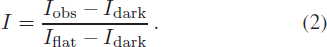
Here, Iflat denotes the flat field (Fig. 2(b)), corresponding to the gains of each detector pixel. Generally, a uniformly illuminating source will not create a uniform output on the CCD due to the flat field. There are several methods to measure the flat field, such as a sky flat, dome flat, Kuhn flat and diffusion plate. Among them, the Kuhn flat is a convenient way to assess flat field measurement, especially for photosphere and chromosphere observations (Kuhn et al. 1991). The accuracy of this flat field is about 0.3% – 1.0% that decided by the sampled offset frames. In our experiments, we only measured nine offset frames. The inhomogeneous large scale pattern can be removed from the nine frames in the offset solar images (right panel in Fig. 3). However, a high frequency pattern still exists. If the small scale stripes are stable, they should be removed with higher frame samples of solar images that are acquired with offset in the point direction. In the following steps, this small scale inhomogeneous problem will be solved with hardware since they change from time to time (probably due to variation in tension of optical glue or air between optical elements).

Fig. 2 Dark and flat frames observed on 2019 February 1. The left panel features the dark frame which manifests residual signals coming from the CMOS camera's eight block readout. The right panel showcases the flat field frame which is calculated from nine offset solar image frames.
Download figure:
Standard image
Fig. 3 Original and flat field processed frames observed on 2019 February 1. The left panel is the original full-disk solar image which contains the ambiguous pattern. The right panel is the dark frame and flat field processed image. In the solar disk center, we can still find some stripes that might come from some tension inside the optical elements (probably glue).
Download figure:
Standard image3.2. Measurement of the Working Line Shifts
Both radial Doppler velocities on the Sun and the wide field of view (WFOV) of instruments can cause shifts of observed spectral lines. The former comes fromlarge-scale solar differential rotation and small-scale plasma motions. A combination of these can result in a Doppler velocity of up to ∼4 km s−1 or even larger. The optical system of the FMG is telecentric, and ideally, all the points in the field of view (FOV) should be treated equally. However, in practice, from the observations by the Huairou full-disk vector magnetograph (Zhang et al. 2007), we found that this design cannot completely reduce variation in the bandpass of the filter at different positions in the image plane. Therefore, we should pay more attention to these two factors in the FMG and carry out measurements in advance.
3.2.1. Radial Doppler velocities
Spectral profiles of the working line were obtained with a set of full-disk 31-step scan filtergrams taken by the Huairou full-disk vector magnetograph, which were observed by scanning the line from its blue wing of −0.3 Å to its red wing of +0.3 Å off the line center in steps of 0.02 Å. Implementing the center of gravity method, we calculated the wavelength shifts at each pixel relative to the solar full-disk center as depicted in Figure 4, in which the maximum value is close to 60 mÅ (velocity ∼vd = 3.4 km s−1). The dividing line between blue and red patches is quite irregular as usual, suggesting that there is another shift caused by the WFOV effect, which will be calibrated on orbit using a method similar to that for the HMI (Couvidat et al. 2012).

Fig. 4 Map of wavelength shifts caused by solar radial Doppler velocities observed with the Huairou full-disk vector magnetograph on 2018 February 13. Note that the shifts, introduced by the WFOV, are not excluded.
Download figure:
Standard image3.2.2. Sun-FMG radial velocity
The FMG onboard the ASO-S satellite is going to work on a Sun-synchronous orbit with an orbital altitude of about 720 km and an orbital inclination angle of 98.27°. The orbital period is about 99.2 min. Figure 5 shows the simulated Sun-FMG radial velocity from Jan. 2021 to Dec. 2021. It can be ascertained that the peak-to-peak value of Sun-FMG radial velocity changes from day to day. During March or October, the Sun-FMG radial velocity is at its lowest, with a peak-to-peak value from −0.52 to +0.52 km s−1 and a period of 99.2 min. The radial velocity reaches its largest during July, a peak-to-peak value from −3.9 to +3.9 km s−1, corresponding to a wavelength shift from −0.07 Å to +0.07 Å away from the working line center. It is worth noting that the radial velocity reaches zero twice in each orbit even if its peak-to-peak value is the largest, due to the sinusoidal variation of the radial velocity in each orbit. So, we have data which are not influenced by the radial velocity about every 49.13 min, which is equal to half of the orbit period.

Fig. 5 Simulated Sun-FMG radial velocity from Jan. 2021 to Dec. 2021.
Download figure:
Standard image3.3. Polarization Crosstalks
Generally, polarimeter calibration of the FMG instrument can disentangle the crosstalks among Stokes parameters effectively (Ichimoto et al. 2008; Schou et al. 2012a). However, on-orbit calibration optics were avoided on the FMG instrument. Also, ground-based calibration may not be able to consider all possible environmental and instrumental drifts. Thus, we develop some methods for data post-processing to complement the drawbacks in the polarimeter calibration. In the current paper, our discussions are limited to the intensity to linear and circular polarizations (Stokes I-to-Q, −U and −V) crosstalks and circular to linear polarization (Stokes V-to-Q and V-to-U) crosstalks introduced by instruments.
3.3.1. Stokes I-to-Q, −U and −V crosstalks
Figure 6(a) and (b) shows the Stokes V images taken at the filter positions ± 0.06 Å observed with the Huairou full-disk vector magnetograph on 2017 September 12. They display brightness in the first and third quadrants and darkness in the second and fourth quadrants, which is caused by Stokes I-to-V crosstalk (Xuan et al. 2010). We select the pixels on the white circle in Figure 6(a) and plot the corresponding signal versus angular position [degrees] in Figure 6(c) and (d) (blue lines). One can see the same periodic and amplitude variation of Stokes V at both wavelength positions. The period is ∼175 deg and the amplitude is ∼ 7 × 10⁻⁴. We chose signals along two white lines (denoted by R1 and R2) to analyze the center-to-limb variation of Stokes V as displayed in Figure 6(e) and (f). We find that Stokes V is more uniform near the solar disk center than it is near the limb. The amplitudes of Stokes V (both negative and positive) start to increase at 200 pixels from the solar disk center. The rate of increase is 3 × 10−6 pixel−1. We also perform the same analysis for Stokes Q and U. The period of Stokes Q is ∼ 450 deg and the amplitude is ∼ 4.6 × 10⁻⁴. The period of Stokes U is ∼ 171 deg and the amplitude is ∼ 2.1 × 10⁻⁴. From the above analysis, we conclude that the Stokes I-to-Q, −U and −V crosstalks are less than 0.1% (∼10 G) of quiet-Sun intensity.

Fig. 6 Distributions of Stokes I-to-V crosstalk. (a) and (b) are the Stokes V images observed at filter positions ∓ 0.06 Å with the SMAT on 2017 September 12, respectively. (c) and (d) are their corresponding azimuthal profiles along the white circle in panel (a). The red lines fit the observed data displayed by the blue lines. (e) and (f) are their corresponding radial profiles along the radial directions, R1 and R2 in panel (a).
Download figure:
Standard imageOne method to obtain the full-disk pattern of intensity to polarization crosstalk is to combine multiple Stokes V/Q/U maps. The average value of Stokes V for 1585 maps is depicted in Figure 7(a), where we apply the threshold 2 × 10⁻³ to remove large V signals. Figure 7(b) displays one Stokes V map before correcting the crosstalk. One can still see alternating bright and dark regions near the solar limb. The result of subtracting Figure 7(a) from Figure 7(b) to correct the Stokes I-to-V crosstalk is shown in Figure 7(c). One can see that Stokes V now has a more uniform background. We select pixels on the green circle in Figure 7(b) to analyze the difference before and after correcting the crosstalk. In Figure 7(d), the blue and red lines represent the Stokes V distribution along the green circle before and after correcting crosstalk respectively. The fitting results are marked by same-colored lines as the observational data. The amplitude of the blue fit line is larger than that of the red one, which indicates that the correction is effective. A similar analysis can be performed for Stokes Q and U, and it is found that this method is also effective for Stokes Q and U.

Fig. 7 Removal of Stokes I-to-V crosstalk. (a) is a full-disk pattern of I-to-V crosstalk obtained by averaging over 1585 images with the threshold value of 2 × 10⁻³. (b) and (c) are the Stokes V images before and after crosstalk removal, respectively. Their corresponding azimuthal profiles along the green circle in panel (b) are shown in (d) with the blue and red lines. The fitting results are also superimposed on the corresponding curves with the same colored lines.
Download figure:
Standard image3.3.2. Stokes V-to-Q and V-to-U crosstalks
Based on an assumption that the Stokes Q and U profiles are symmetric and V profile is anti-symmetric, the coefficient of V-to-Q (U) crosstalk, Cq (Cu), is given by the ratio of the difference of a pair of Q (U) maps taken at symmetric line wings off the line center to that of a pair of V maps (Mickey 1985; West & Balasubramaniam 1992). With this method, Su & Zhang (2007) obtained the solar full-disk maps of Cq and Cu. However, due to the effects of radial Doppler velocities, the above-mentioned signals of Q (U) maps cannot be measured exactly at any symmetric line wings of the working line unless Q, U and V profiles are available.
Therefore, the data of 31-step scan filtergrams that are described in Section 3.2.1 are used to determine the line centers in each pixel, and then the data of the 31-step scan Stokes Q, U and V profiles are employed to find symmetric line wing positions off the determined line centers, e.g., ± 0.08 Å. Finally, Cq and Cu maps can be measured as shown in Figure 8. They are the averaged results of 17 sets of Cq and Cu maps taken from 2017 June 19 to 2018 February 11 and in this way the environmental drifts are excluded as much as possible. The maximum values of V-to-Q and −U crosstalks are up to ∼ 17% and ∼ 22%, respectively. Also, Cq and Cu maps exhibit a regular distribution over the entire FOV. Two nearly symmetric red patches are aligned along the X-axis direction and two blue ones are aligned along the Y-axis direction in Figure 8(a). It seems that if they are rotated 45° clockwise, in terms of morphology they become the plot of Figure 8(b). In addition, we found that the averaged Cq and Cu maps as depicted in Figure 8 cannot be used to remove V from Q and U signals taken on a specific day. This indicates that the environmental drifts should take effect in the ground-based polarization crosstalks. Figure 9 displays the raw and corrected data of the Stokes Q and U full-disk maps observed on 2017 September 29 and the maps of Cq and Cu maps measured on the same day.

Fig. 8 Full-disk maps of the coefficients of Stokes V-to-Q and −U crosstalks. To remove environmental drifts, they are obtained by taking an average over 17 sets of Cq and Cu maps acquired from 2017 June 19 to 2018 February 11.
Download figure:
Standard image
Fig. 9 Maps of Stokes Q and U observed on 2017 September 29. The raw data are shown in the top two panels and the corrected data in the bottom two panels.
Download figure:
Standard image3.4. Inversions of Magnetic Fields
For routine observational mode in the future, the FMG plans to take Stokes Q, U and V signals at only one wavelength position of the working line. Correspondingly, calibrations of magnetic fields are to be performed at the same position. However, for some special observational modes, two symmetric wavelength positions or the whole spectral line may also be employed. Therefore, calibrations at two symmetric wavelength positions and magnetic field inversion with the whole line profiles should be studied in advance.
3.4.1. Linear calibration in the weak-field approximation
When the Zeeman splitting vb is small enough, its two components can be written in the form (Jefferies et al. 1989)
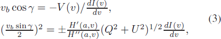
where γ is the angle between the line of sight and the magnetic field B, a is the damping parameter, v is the dimensionless wavelength shift and H(a,ν) is the Voigt function. Clearly, as vb ∼B, Equation (3) thus constructs a direct connection between longitudinal (BL) and transverse (BT) fields with Stokes parameters under the weak-field approximation, which are
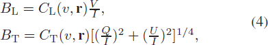
where CL and CT are functions of both longitudinal and transverse spatial positions. At the wavelength position of −0.08 Å off the line center, the linear calibration errors are ∼ 10 G and ∼ 15 G for BL = 2165 G and BT = 1250 G (Su & Zhang 2007), respectively. CL and CT connect with spatial positions arising from radial Doppler velocities on the solar full-disk and the effects of instrument WFOV, which lead to wavelength shifts shown in Figure 4.
To study the impacts of wavelength shifts on Stokes I, Q, U and V parameters,we simulated them by numerically solving Unno-Rachkovsky equations for the polarized radiative transfer of the working line (Ai et al. 1982). We utilized the vector field parameters B = 2000 G, γ = 30° and the azimuth λ = 45°. The heliocentric angle μ is obtained with the formula

where L0 and B0 are the heliographic longitude and latitude at the disk center, and L and B are those at the other disk positions. The map of μ was calculated with respect to the time 23:53:15 UT on 2019 April 3. Thus, we downloaded a Dopplergram of HMI at the same time to modify the simulated full-disk maps of Stokes parameters, the Stokes I maps of which the are shown in Figure 10 at the blue wing of −0.08 Å and the red wing of +0.08 Å off the line center. Figure 11 shows the extracted data along the white line as depicted in Figure 10(a). As expected, Stokes parameters are not affected by the radial Doppler velocities around the disk center. However, away from this region, Stokes I manifests almost linear variation at both line wings while Q, U and V exhibit nonlinear variations. From the disk center to its limbs, we estimate that the varying amplitudes are ∼29%, 16%, 44% and 50% for Stokes I, Q, U and V, respectively.

Fig. 10 Simulations of the full-disk maps of Stokes I at the offset position of −0.08 Å (a) and +0.08 Å (b) of the working line. They were modified by the solar differential rotation at 23:53:15 UT on 2019 April 3.
Download figure:
Standard image
Fig. 11 Simulated signals of Stokes I, Q, U and V at ± 0.08 Å (blue: −0.08 Å red: +0.08 Å) off the working line center located along the white cut running through the full-disk center as depicted in Fig. 10(a).
Download figure:
Standard image3.4.2. Calibration at one wavelength using machine learning
For filter-based magnetographs, the linear magnetic field calibrationmethod under the weak-field assumption is usually adopted. This leads to the existence of the magnetic saturation effect in the magnetic field. As a typical algorithm for traditional multi-layer network training, a backpropagation (BP) neural network has a relatively simple structure. It is a good network for an initial attempt at single-wavelength magnetic field calibration.
We explore a BP neural network with one input layer, five hidden layers and one output layer, using data from the Spectro-Polarimeter onboard Hinode (Hinode/SP) to simulate single-wavelength observations for model training, comprehensively considering the influence of Doppler velocity field and filling factor. The linear fitting coefficient between the training result and the target on the transverse field is able to reach above 0.96, and that on the longitudinal field above 0.99. We confront the BP neural network with linear calibration, pointing out that the BP neural network performs better at correcting the magnetic saturation effects as shown in Figure 12. The errors are typically about 20G and 60G less than linear calibration on the transverse field and longitudinal field, respectively. In addition, we found that there are many "bright spots" on the inclination from Hinode/SP inversion data with a value of 180 deg, which may be caused by non-convergence in the Stokes inversion process, and the BP neural network could generalize these points well as shown in Figure 13.

Fig. 12 Comparisons between Stokes inversion, BP neural network model training and linear calibration. From top to bottom, they are the results of Stokes inversion, BP neural network model training and linear calibration respectively. Left panels present transverse field and right panels longitudinal field.
Download figure:
Standard image
Fig. 13 Comparisons between Stokes inversion and BP neural network model training on the field inclination. The Stokes inversion results are on the left and the BP neural network model training results are on the right.
Download figure:
Standard imageHowever, we emphasize that this method is only a preliminary attempt and is an auxiliary means at present, which cannot replace the linear calibration. In short, we develop a non-linear method which can be used for magnetic field calibration for filter-type magnetographs.
3.4.3. Calibration at two symmetric wavelength positions
Su & Zhang (2007) have demonstrated that summations of a group of Stokes I/Q/U/V parameters at two symmetric positions can remove Stokes I-to-V and V-to-Q/U crosstalks. In addition, we found that from the disk center to the solar limb, the variations in amplitude of the combined I', Q', U' and V' are ∼ 2%, 7%, 11% and 14%, respectively, as depicted in Figure 14. These are significantly lower than the same values at only one wavelength position (see Sect. 3.3.1). For convenience, in the figure light blue plus symbols displaying the combined data are named Data I, orange plus symbols displaying Data I smoothed over a boxcar o 72'' × 72'' as Data II and deep blue plus symbols displaying Data I divided by Data II and then normalized as Data III. In addition, if Data II are calibrated into magnetic fields (BX, BY and BL), we then name them Data IV. Figure 15 features Data IV (already normalized) varying with different input B values (500 – 2500 G). These profiles almost coincide around the disk center and gradually differ close to the solar limb. However, the largest difference is ∼ 2% or so. This indicates that we may create full-disk maps of averaged Data IV over 500 – 2500 G to correct vector magnetograms, in other words, to correct for large-scale solar differential rotation. The correction error is estimated to be ∼ 2% in the range 500 – 2500 G.

Fig. 14 Combinations of a group of Stokes I/Q/U/V parameters as shown in Fig. 11. They are in turn (I−0.08 + I+0.08)/2, (Q−0.08 + Q+0.08)/2, (U−0.08 + U+0.08)/2 and (V−0.08 − V+0.08)/2.
Download figure:
Standard image
Fig. 15 Variations of Data IV with the input parameter of magnetic field strength B.
Download figure:
Standard image3.4.4. Stokes inversion based on the scanned spectral profiles
The transmission profile for the Lyot filter of the FMG can be tuned to different wavelength positions within its spectral free range. If we carry out polarization observations at each wavelength position, the Stokes I, Q, U and V profiles of the working line can be obtained. Once we have found the Stokes profiles, the vector magnetic fields can be derived by applying a suitable Stokes inversion technique. In this case, the calibration error of the vector magnetic fields is lower relative to the calibration based on the observations at single or two wavelength positions. For the FMG, we plan to tune the Lyot filter on orbit and obtain and obtain Stokes I, Q, U and V profiles from time to time with the calibration mode. The vector magnetic fields, on the basis of these data, can further be used to construct the sample set for the magnetic field calibration at a single wavelength, corresponding to the data taken in the routine mode.
As an example, Figure 16 plots the Stokes I, Q, U and V profiles from one pixel of an active region observed with the Huairou full-disk vector magnetograph on 2017 September 7. The polarization data are observed by scanning the line from its blue wing of −0.3 Å to the red wing of +0.3 Å off the line's center in steps of 0.02 Å. The solid lines in Figure 16 represent the fitting results with Milne-Eddington Solar Atmosphere Inversion Library (MEINV) code, which is developed by Teng & Deng (2014) and implemented for Stokes inversion with the Solar Magnetic Field Telescope (SMFT) in Huairou Solar Observing Station (HSOS) (Bai et al. 2014).MEINV code is based on the Levenberg-Marquardt least-squares fitting algorithm to invert magnetic field parameters from the Stokes I, Q, U and V profiles, adopting the analytical solution under the assumption of the M-E atmosphere model. In Figure 17, we also present the full-disk magnetic field strength, inclination angle and azimuth angle fromthe inversion.

Fig. 16 Observational Stokes I, Q, U, V profiles (plus symbol) and their inversion results (solid line) with MEINV code. The observational data come from the Huairou full-disk vector magnetograph, and were observed by scanning the line from its blue wing of –0.3 Å to the red wing of +0.3 Å off the line center in steps of 0.02 Å.
Download figure:
Standard image
Fig. 17 Full-disk magnetic field strength, inclination angle and azimuth angle obtained with the inversion technique for Stokes Q, U and V parameters on the basis of the data taken on 2017 September 7.
Download figure:
Standard image4. Data deep reduction
4.1. 180-degree Ambiguity
In the measurement of vector magnetic field, one of the well-known problems is the 180° ambiguity in the measured transverse field. There are two possible orientations with a difference of 180° for the transverse field vector. Before calculating any physical quantities of the vector magnetic field, this 180° ambiguity must be resolved. Metcalf et al. (2006) and Leka et al. (2009) introduced several approaches and quantitatively compared the algorithms which are used to solve the ambiguity. There are five basic methods: the acute angle method, large scale potential method, uniform shear method, magnetic pressure gradient method and minimum energy method. We introduce the acute angle method and minimum energy method in the following paragraphs.
The acute angle method resolves the 180° ambiguity by comparing the observed transverse field with an extrapolated transverse field. When the observed field and extrapolated field make an acute angle, i.e., −90 ° ≤ Δ θ ≤ 90 ° (Δ θ = θo − θe), the direction of the transverse field is determined by the extrapolated field direction. This condition can be expressed as  , where
  is the observed transverse component and
  is the extrapolated transverse component.
The minimum energy algorithm minimizes both the electric current density J and magnetic field divergence simultaneously. Originating from Aly (1988), magnetic free energy is proportional to the maximum value of J2/B2 for a force-free field. Given this, Metcalf (1994) named this method the minimum energy algorithm. Based on the equation ∇ · B = 0 and the observed electric current density J, they defined the energy as E = ∑(|∇ · B| + |J|)2. In this method, the minimum energy E should be calculated to resolve the 180° ambiguity. The transverse ambiguity of SDO/HMI was solved by applying this method (Bobra et al. 2014).
4.2. Projection Correction
The projection correction includes two aspects: remapping and vector transformation. The former involves coordinate changes from 2D observing coordinates into 3D spherical coordinates, and the latter presents vector fields in spherical coordinates (Sun 2013). As with the HMI remapping, the FMG first uses a cylindrical equal area (CEA) projection (Calabretta & Greisen 2002) to mitigate the foreshortening effect, and then converts the Heliographic Coordinates (ϕ, λ) to CCD coordinates (ξ, η). Figure 18 displays an example of remapping a longitudinal magnetogram that was taken on 2017 September 3. Clearly, this remapping is undistorted along the equator, but the distortion increases rapidly towards the poles. Lastly, we removed one patch (AR 12674) from the whole FOV as shown in Figure 18(a) to perform vector transformation. Three components of vector magnetic fields (Bξ, Bη, Bζ) are disentangled with respect to 180° ambiguity using the potential field acute angle method. They are transformed to (Br, Bθ, Bϕ) following equation (1) in Gary & Hagyard (1990) and the results are shown in Figure 19.

Fig. 18 Remapping of a longitudinal magnetogram with CEA projection.
Download figure:
Standard image
Fig. 19 Vector magnetogram of AR 12674 on 2017 September 3. Panel (a) is the original vector magnetogram with projection and panel (b) is the one with projection removed.
Download figure:
Standard image5. Conclusions
This paper describes the details of the FMG data analysis, which may be further improved and become the FMG processing pipeline after the ASO-S is launched. No doubt, the analysis will be helpful for future polarizationmeasurements with the required accuracy.We have gained valuable insights for future space-based data analysis.
Acknowledgements
We greatly appreciate constructive discussions with Prof. Yang Liu and are indebted to Dr. Xudong Sun for valuable suggestions. This work is supported by the Strategic Priority Research Program on Space Science, the Chinese Academy of Sciences (Grant Nos. XDA15320302,XDA15052200 and XDA15320102), the National Natural Science Foundation of China (Grant Nos. 11773038, 11703042, U1731241, 11427901, 11427803, 11473039 and U1831107), and the 13th Fiveyear Informatization Plan of the Chinese Academy of Sciences (Grant No. XXH13505-04).