


Abstract
When multiphase flows are modeled numerically, complex geometrical and operational features of the experiments, such as the phase mixing section, are often not resolved in detail. Rather simplified boundary conditions are prescribed, which usually cause less irregular dynamics in the system than present in reality. In this paper, a perturbation that randomly disturbs the secondary components of the velocity vector at the inlet is proposed in order to capture the experimentally observed instabilities at the interface between the phases. This in particular enhances the formation of slugs in the pipe. Different amplitudes of the perturbation are investigated. One observes that, the higher the perturbation amplitude, the earlier the slugs occur. On the other hand, sufficiently far away from the inlet, the flow pattern shows the same dynamics for different perturbation amplitudes. Hence, no specific frequency is imposed by the prescribed perturbation. The simulation results are validated by comparison with liquid level data from a corresponding experiment.
Export citation and abstract BibTeX RIS

Original content from this work may be used under the terms of the Creative Commons Attribution 4.0 licence. Any further distribution of this work must maintain attribution to the author(s) and the title of the work, journal citation and DOI.
1. Introduction
Computational fluid dynamics (CFD) has already proven to be a useful tool for the modeling of single-phase flow metering [1]. It has been used to estimate systematic contribution to measurement uncertainty due to installation effects of flow meters [2], Bayesian uncertainty evaluation in measurements based on reconstruction of flow profiles [3], and as crucial tool for uncertainty evaluation in specific applications [4]. CFD calculations also were employed in realistic simulation measurement set-ups in order to ensure suitable measurement conditions, e.g., in a gas-mixing unit [5], to predict flow profiles in specific situations [6], or to explore the effect of flow conditioning elements [7].
The measurement of multiphase flow, especially two-phase gas-liquid flow, is of great importance for a variety of applications and industrial processes, for example in nuclear, chemical, or oil and gas industries [8, 9]. The complexity of multiphase flow measurement arises not only due to indirect measurement methods using technologically advanced meters based on sophisticated mathematical models, but also due to specific multiphase flow phenomena such as different flow regimes [10, 11]. Therefore, the urgent need for improvement of multiphase flow measurement accuracy requires a better understanding of multiphase flow behavior in the measurement system. CFD simulations of multiphase flows with different properties and at different flow rates promise to elucidate and quantify the influence of these flow conditions on the actual process of measurement.
In the last decades, several mechanistic models and empirical correlations of two-phase gas-liquid flow were developed to predict the characteristics of slug flow based on superficial velocities, fluid properties, and pipe geometry [12–20]. More recently, CFD was used to predict the different flow patterns in horizontal gas-liquid two-phase flow. One of the first attempts was done by Lun et al [21]. The authors simulated horizontal two-phase flow using a commercial CFD package. Over the last 20 years, the use of CFD for multiphase flows has increased significantly. There are a lot of publications on the numerical simulation of gas-liquid flow in horizontal pipes [22–33].
Nevertheless, the simulation of slug flow is still a research topic. Numerical simulations are very time-consuming since transient simulations with small time step sizes are necessary. In addition, pipes need to have sufficient length for slug flow to evolve. Fine grids are required in order to resolve the instabilities at the interface between the phases, which are responsible for the development of slugs in the pipe. This leads to a high consumption of memory for the simulations. Therefore, there is a need to understand, how the development of slugs can be enhanced in the numerical simulation.
Frank [22] investigated air-water slug flow in a horizontal pipe by means of transient 3D simulations. He prescribed a sinusoidally varying liquid level at the inlet of the pipe to enhance the development of slugs. Later, Ban et al [31] used a similar approach and prescribed a transient liquid level at the inlet cross section of the pipe. However, a drawback of these approaches is that the prescribed agitation frequency is reflected in the frequency of slug occurrence further downstream in the pipe. In appendix
In this paper, we introduce a perturbation, which randomly disturbs the secondary components of the velocity vector at the inlet. We show that, such a perturbation enhances the evolution of slugs in the pipe. The higher the amplitude of the perturbation, the earlier slugs occur in the pipe. On the other hand, further downstream in the pipe, the mean slug frequencies for the different perturbation amplitudes converge to one common slug frequency. Therefore, it can be concluded that, at sufficient distance from the inlet, the main features of the flow are not affected by the amplitude of the perturbation. In addition, the proposed perturbation does not force periodic slug flow as it is the case for the perturbation proposed earlier by Frank [22]. Hence, it can also be applied to model non-periodic slug flow.
2. Methods
In this section, we describe the experimental and numerical set-up of the considered slug flow and introduce the methods needed for the analysis.
2.1. Experimental set-up
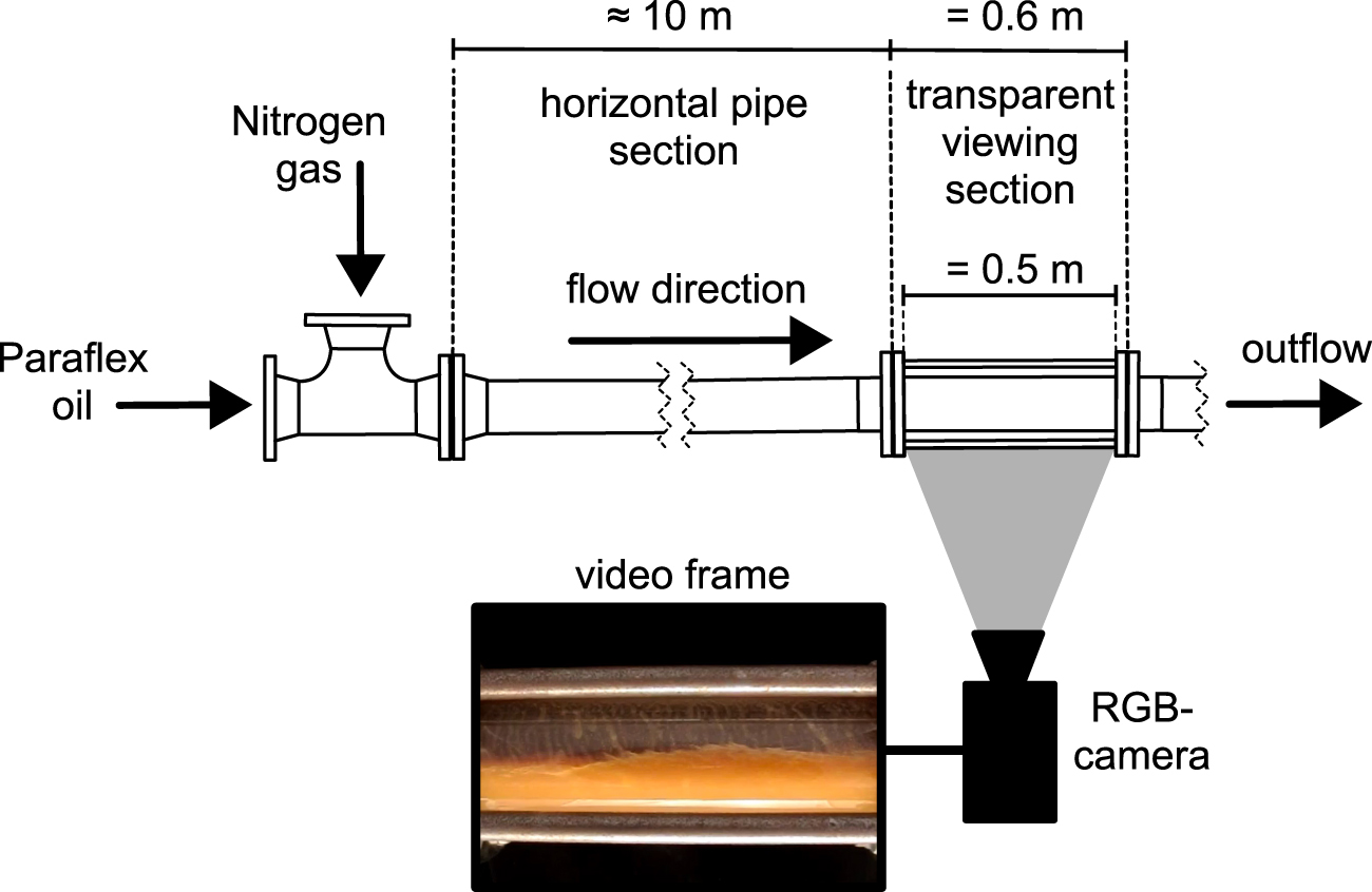
The experimental data of a horizontal gas–liquid slug flow are used to verify the numerical model and the developed inlet-perturbation described later in the text. The experiment was performed by TÜV SÜD National Engineering Laboratory (NEL) as part of the project Multiphase flow metrology in oil and gas production [34]. The experimental set-up is illustrated in figure 1. It consists of a straight horizontal pipe with an inner diameter of D = 0.097 18 m and a length of approximately 10 m, followed by a transparent Perspex viewing section with a length of 0.5 m, where the slug flow was recorded from the side by a high-speed RGB-camera (Casio EX-10) with a frame rate of 240 fps. The spatial resolution of the system was 512 × 384 pixel.

Figure 1. Illustration of the experimental set-up with high speed video recording.
Download figure:
Standard image High-resolution imageThe fluid properties and superficial velocities of the experimental slug flow are summarized in table 1.
Table 1. Fluid properties and superficial velocities of the considered slug flow.
| Paraflex oil | Nitrogen | |
|---|---|---|
Density in 
| 815.83 | 10.8 |
| Dyn. viscosity in Pa ⋅ s | 7.836 × 10⁻³ | 1.75 × 10⁻⁵ |
Surface tension in 
| 0.028 58 | |
Superficial vel. in 
| 1.873 | 0.624 |
2.2. Numerical set-up
For a better assessment of the development of slug flow, a longer pipe (L = 16 m ≈ 165D) than in the experiment is considered in the numerical simulation, see figure 2. If no perturbation is used, such a long pipe is needed for the development of slug flow in the numerical simulation because of the simplified modeling of the inlet boundary conditions.

Figure 2. Illustration of the geometry and initialization for the numerical simulation.
Download figure:
Standard image High-resolution imageIn the following, we first introduce the mesh used for the simulations. Then, we define the random perturbation as well as the other initial and boundary conditions. Finally, the numerical discretization schemes are summarized.
2.2.1. Mesh design
In order to ensure mesh independent results, four o-grid type meshes were generated using the utility blockMesh, supplied with OpenFOAM®. The corresponding number of cells per diameter and per one meter in the direction of the flow are summarized in table 2. Note that, the meshes m3 and m4 were designed as only one half of the geometry with a symmetry plane in the y-axis, see figure 2. Since the flow structures observed in the simulation of the complete geometry show a symmetrical behavior, this simplification is supposed to not influence the resulting flow pattern.
Table 2. Mesh parameters.
| Number of cells in mesh | m1 | m2 | m3 | m4 |
|---|---|---|---|---|
| Per diameter | 32 | 46 | 60 | 70 |
| Per meter in length | 80 | 100 | 150 | 200 |
Figure 3 shows the velocity profiles and liquid phase fraction at x = 5 m averaged over a time interval of 5 s. As a compromise between time expenses and accuracy, mesh m3 was selected for further investigations. In total, this mesh consisted of approximately 2.8 million cells. The first quadrant of the pipe cross section of mesh m3 is illustrated in figure 4.
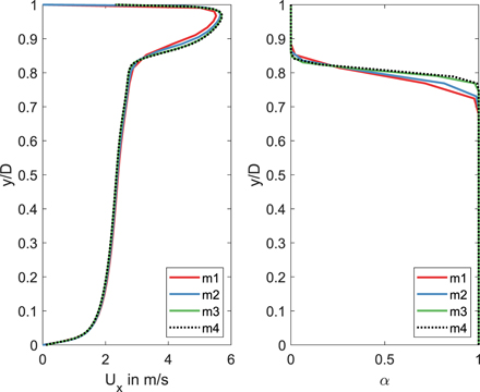
Figure 3. Time-averaged velocity profiles and liquid phase fraction α at x = 5 m in dependence on the used mesh.
Download figure:
Standard image High-resolution image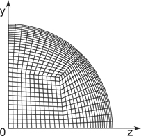
Figure 4. Illustration of first quadrant of the pipe cross section of the mesh m3.
Download figure:
Standard image High-resolution image2.2.2. Boundary conditions and random perturbation
The inlet cross section was bisected horizontally as indicated in figure 2. In the lower half, the liquid volume fraction, α, was set to 1. In the upper half, it was set to 0. For t = 0, it was assumed that the pipe is only filled with gas. Altogether, this leads to the following initial and boundary conditions for α:

The boundary conditions for the velocity are as follows. At the inlet (x = 0), we prescribed twice the superficial velocities for the x-component, Ux , in each phase:

Here, Usg and Usl denote the gas and liquid superficial velocities, respectively. For the y- and z-components, Uy and Uz , random perturbations were defined as follows:


where Δy (t) and Δz (t) denote the displacement of the velocity vector in y- and z-direction in polar coordinates, i.e.,

The random parameters r(t) and ϕ(t) are assumed to be uniformly distributed:

Here, ![$\mathcal{U}\left[a,b\right]$](https://content.cld.iop.org/journals/0026-1394/58/1/014003/revision4/metabd1c9ieqn4.gif) denotes the uniform distribution over the interval
denotes the uniform distribution over the interval ![$\left[a,b\right]$](https://content.cld.iop.org/journals/0026-1394/58/1/014003/revision4/metabd1c9ieqn5.gif) . The parameter Rpert determines the maximal possible amplitude of the perturbation. In the following, Rpert is set to 0.025, 0.05, 0.1, 0.2, and 0.4. This corresponds to a perturbation of the velocity vector in y- and z-direction of maximally 2.5, 5, 10, 20, and 40 per cent of the velocity in flow direction.
. The parameter Rpert determines the maximal possible amplitude of the perturbation. In the following, Rpert is set to 0.025, 0.05, 0.1, 0.2, and 0.4. This corresponds to a perturbation of the velocity vector in y- and z-direction of maximally 2.5, 5, 10, 20, and 40 per cent of the velocity in flow direction.
At the outlet, a constant pressure boundary condition was used. The walls were treated as hydraulically smooth with classical no-slip boundary conditions.
2.2.3. Numerical schemes
For the numerical simulation, the software package OpenFOAM-5.x was used. From this package, the two-phase solver interFoam was chosen, which is designed for transient simulations of two incompressible, isothermal immiscible fluids and is based on the volume of fluid (VOF) method [35]. The VOF method is a numerical technique for tracking and locating the interface between the two fluids. The solution procedure involves the MULES (multidimensional universal limiter with explicit solution) method to keep the VOF data bounded. The pressure-velocity coupling is computed by the PIMPLE algorithm, a combination of the PISO (pressure-implicit with splitting of operators) algorithm and SIMPLE (semi-implicit method for the pressure linked equations) algorithm. A comprehensive description of the interFoam solver can be found in [36].
Since the flow rates indicate a turbulent flow regime, Menter's shear stress transport (SST) turbulence model was applied for closing the Reynolds-averaged Navier-Stokes (RANS) equations [37]. For the time discretization, the implicit Euler scheme was used. The time step size was adjusted automatically by limiting the Courant number to 0.5. For the considered slug flow, this leads to an average time step size of about 3 × 10⁻⁴ s. The schemes used for the spatial discretization are summarized in table 3.
Table 3. Schemes used for the spatial discretization of the gas–liquid slug flow with OpenFOAM.
| Scheme | Method |
|---|---|
| Gradient | Gauss linear |
| Laplacian | Gauss linear corrected |
| Divergence | Gauss van Leer/Gauss linear |
2.3. Methods for data analysis
In the following, we introduce the methods used for the analysis of the results. First, it is described how the liquid level time series were extracted from the experimental video observations as well as from the simulation results. Afterwards, we introduce the slug characteristics that are used in the paper. Finally, the frequency analysis and its parameters are summarized.
2.3.1. Extraction of liquid level time series
For the validation of the simulated slug flow with the experimental slug flow, the time series of the vertical position of the gas-liquid interface at a certain x-position are considered. This non-dimensional parameter represents the dynamics of the gas-liquid flow pattern and has a range of [0, 1] with respect to the inner pipe diameter D. It is hereinafter also referred to as the liquid level time series at a certain x-position, denoted by hl(x, t).
For the experimental data, the liquid level time series are extracted from high speed video observations. Here, the video observations represent a two-dimensional projection of the three-dimensional flow from the side, i.e., in the x–y plane. To extract the liquid level time series from the video, an image processing routine is used, which was developed in our earlier work [38]. Since the flow is observed through a transparent Perspex pipe wall with a thickness of 0.0214 m, the liquid level observed from outside is distorted in y-direction compared to the real liquid level inside the pipe. Therefore, a correction was applied, which is based on Snell-Descartes law and trigonometry. Details on this correction algorithm can be found in our earlier work [39]. The slug flow was recorded for approximately 122 s. Note that, only 94% of the inner diameter of the pipe are visible in the experimental observation, due to the construction of the Perspex viewing section. The lowest and highest 3% of the pipe cannot be seen because of tie bars that were needed for the installation of the Perspex pipe section. Nevertheless, the liquid level time series extracted from this observation represents the dynamics of the gas-liquid interface and reveals temporal characteristics of the flow structures, such as slugs or waves.
From the simulation results, the liquid level time series at a fixed position x are approximated for all t ∈ [t1, t2] by the mean value of the liquid volume fraction α over the vertical line in this cross section through the middle of the pipe:

For the analysis of the simulation results, we considered a time interval of 50 s (t1 = 10 s, t2 = 60 s). Note that, the chosen time interval is large enough that there is no dependency of the results on time. This was checked by subdividing the considered time interval into two smaller intervals of half size and comparing the results on these intervals with each other. It was found that, for the two intervals [10 s, 35 s] and [35 s, 60 s], the absolute error of the mean values was lower than 0.0022 for all x-positions (x ∈ {6 m, 8 m, ..., 14 m}) and all perturbation amplitudes (Rpert ∈ {0, 0.025, 0.05, 0.1, 0.2, 0.4}). For the standard deviations, the absolute error was below 0.0066 for all cases.
2.3.2. Slug characteristics
Slug flow is characterized by a continuous liquid phase with coherent blocks of aerated liquid called slugs, which are separated by volumes of gas and moving on top of a slowly flowing liquid layer downstream the pipe at approximately the same velocity as the gas [12, 20, 40], as shown in figure 5. Slugs are typically quantified by their length and time scales, such as the slug body length Lb, the slug unit length Ls, the time of a slug body passing by at a fixed position Tb and the time of a slug unit passing by at a fixed position Ts [41, 42]. The slug unit with corresponding length and time scales is illustrated in figure 5. Note that Lb is related to Tb and Ls is related to Ts with the use of corresponding translational velocities. In the following, Tb will be referred to as slug body time and Ts will be called slug unit time. Based on the slug unit time, Ts, the slug frequency is given by  . Then, the mean or averaged slug frequency can be calculated by

where Ns denotes the number of slugs in the considered time interval [43].

Figure 5. Illustration of a slug unit (left) with length scales and corresponding liquid level time series (right) extracted at position x of the pipe with time scales.
Download figure:
Standard image High-resolution imageFor the analysis of the slug flow in this contribution, the focus is on the time scales and interface dynamics, derived from the liquid level time series. To detect the slug fronts and slug rears in the liquid level time series, a threshold for hl is set, as illustrated in figure 5. This threshold needs to be chosen carefully and individually for all time series. It should not be too high, otherwise larger slugs are separated by their entrained gas bubbles. However, it should be high enough to avoid the detection of large amplitude waves.
2.3.3. Frequency analysis
For the frequency analysis, time series of the liquid level at different x-positions in the pipe were considered. Fast Fourier transform (FFT) as well as Welch's power spectral density (PSD) estimate (function pwelch in Matlab) were applied. The function pwelch calculates the one-sided PSD estimate using Welch's segment averaging estimator, see [44] for details. Due to additional smoothing, it is more robust than a pure FFT. Table 4 summarizes the parameters used for the computation of pwelch. In the simulation, data were saved every 0.0025 s leading to a sampling frequency of 400 Hz. In the experiments, data were sampled with a frequency of 240 Hz. For both, simulation and experimental data, the segment length of the filter corresponds to a time interval of 2 s. The number of discrete Fourier transform (DFT) points corresponds to a time interval of 20 s.
Table 4. Parameters used for the calculation of pwelch.
| Parameter | Sim. data | Exp. data |
|---|---|---|
| Sampling frequency | 400 Hz | 240 Hz |
| Segment length | 800 | 480 |
| Overlap | 0 | 0 |
| Number of DFT points | 8000 | 4800 |
3. Results and discussion
In this section, we present simulation results showing the influence of the random perturbation on the evolution of slugs in the pipe. First, we show snapshots of the flow pattern observed for different amplitudes of the perturbation. It can be seen that, the higher the perturbation amplitude, the earlier slugs occur in the pipe. Next, results of the frequency analysis of the liquid level time series are presented. The analysis shows that, in sufficient distance from the inlet, the dominant frequencies are independent of the perturbation amplitude. Finally, the evolution of slugs in the pipe is investigated. For this, the time scales Ts and Tb (see figure 5 for illustration) as well as the mean slug frequency  , see equation (8), are examined.
3.1. Influence of the perturbation amplitude on the development of slugs in the pipe
Figure 6 shows snapshots of the simulated slug flow at time t = 6.5 s for the different amplitudes. These snapshots are gas volume fraction fields in a longitudinal section through the middle of the pipe (z = 0) between x ≈ 9 m and x ≈ 14 m. Without perturbation (Rpert = 0), one cannot observe any slugs in the shown section of the pipe (see top picture in figure 6). In this case, the slugs are formed further downstream than 14 m. For a perturbation amplitude of Rpert = 0.025, slug flow can be observed approximately 10.75 m downstream of the inlet. For higher amplitudes, the onset of slug initiation occurs further upstream. For Rpert = 0.025, Rpert = 0.05, and Rpert = 0.1, narrow slug precursors are visible between x ≈ 9.5 m and x ≈ 11 m and larger slugs can be observed further downstream in the pipe. This illustrates how the slugs grow when travelling downstream the pipe. Based on this slug growth, it can be concluded that the slugs appearing larger in the snapshots were formed further upstream the pipe compared to the ones that appear smaller. Altogether, one observes that, the higher the amplitude of the random perturbation at the inlet, the earlier slugs occur in the pipe.

Figure 6. Snapshots of the resulting slug flow pattern in a longitudinal section through the middle of the pipe (z = 0) for different perturbation amplitudes. Note that, the pictures are not to scale.
Download figure:
Standard image High-resolution imageFigure 7 shows the mean value (a) and standard deviation (b) of the liquid level time series at different cross sections between x = 6 m and x = 14 m for different perturbation amplitudes. In figure 7(a), one observes a decrease in the mean liquid level from approximately 0.80 to 0.78 for all amplitudes. This decrease indicates the development of the slug flow and can be explained as follows. As long as there are no slugs in the pipe, the gas phase flows with a much higher velocity than the liquid phase. When slugs are formed, they block the gas flow. Thus, the gas phase is decelerated. Furthermore, the liquid slugs are accelerated by the faster gas flow. Therefore, due to conservation of mass, the mean liquid level decreases during slug flow. The larger the perturbation amplitude, the earlier the decrease of the liquid level occurs. This shows that the random perturbation enhances the development of slug flow in the pipe. For the simulation without perturbation (Rpert = 0), no slug flow is observed between x = 6 m and x = 14 m. Therefore, we additionally extracted the liquid level time series for x = 15 m, where slugs can be observed in the snapshots of the gas volume fraction fields (not shown). As expected, the mean liquid level decreases for Rpert = 0 at x = 15 m indicating the onset of slug flow.
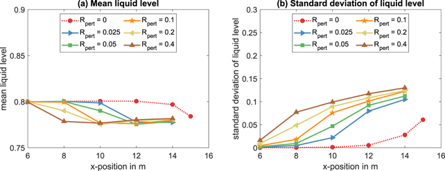
Figure 7. Mean value (left) and standard deviation (right) of the liquid level time series at different cross sections between x = 6 m and x = 14 m for different perturbation amplitudes Rpert ∈ {0, 0.025, 0.05, 0.1, 0.2, 0.4}. For Rpert = 0, data for x = 15 m are additionally shown.
Download figure:
Standard image High-resolution imageFigure 7(b) shows an increase in the standard deviation of the liquid level for all perturbation amplitudes. The higher the perturbation amplitude, the faster this increase occurs. Since the standard deviation still changes at position x = 14 m, it can be concluded that the slug flow in the pipe is still evolving.
3.2. Frequency analysis of the liquid level time series
In the following, a frequency analysis of the liquid level time series is performed in order to determine the dominant frequencies of the interface dynamics. Considering the evolution of the flow pattern downstream along the pipe, one observes the following stages: (1) stratified flow, (2) development of waves, (3) wave growth and slug precursors, and (4) slug flow. The position, where the flow changes from one pattern to another, is influenced by the amplitude of the perturbation prescribed on the inlet. The higher the perturbation amplitude, the earlier these changes occur. Figure 8 illustrates this observation. It shows the PSD of the liquid level time series at position x = 10 m for two different perturbation amplitudes, Rpert = 0.025 (left picture) and Rpert = 0.2 (right picture), which correspond to two different stages of the evolving flow pattern. For Rpert = 0.025, the flow is still wavy at x = 10 m, whereas for Rpert = 0.2, slugs can already be observed at this position. For wavy flow, the corresponding amplitudes of the PSD are more than an order of magnitude smaller (see left picture in figure 8) than for slug flow (see right picture in figure 8). This significant difference can be explained by the fact that for slug flow there is more power present in the time signal than for wavy flow. On the other hand, considering the frequencies that correspond to the highest peaks in the PSD, one observes a decrease for higher perturbation amplitudes. Therefore, the occurrence of slug flow in the pipe can also be detected by considering the most dominant frequencies of the FFT/PSD spectra at different downstream positions and comparing them with each other.
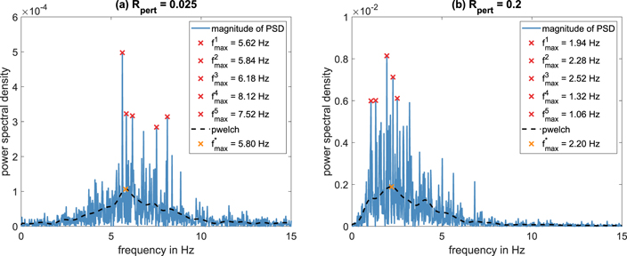
Figure 8. Frequency analysis of the liquid level time series at x = 10 m for two different perturbation amplitudes (left: Rpert = 0.025, right: Rpert = 0.2). Blue line: magnitude of PSD, red crosses: five highest peaks of PSD and corresponding frequencies, dashed black line: Welch's PSD estimate, yellow cross: highest peak in Welch's PSD estimate and corresponding frequency.
Download figure:
Standard image High-resolution imageFigure 9 shows the dominant frequencies derived by FFT (a) and pwelch (b) of the liquid level time series at different cross sections between x = 6 m and x = 14 m for the perturbation amplitudes Rpert ∈ {0.025, 0.05, 0.1, 0.2, 0.4} and between x = 6 m and x = 16 m for Rpert = 0. In figure 9(a), a drop of the frequencies from approximately 4 Hz to 7 Hz down to 2 Hz and less can be observed for all perturbation amplitudes. Since the corresponding amplitudes of the FFT are much lower for the higher frequencies than for the lower ones, it can be concluded that the higher frequencies obtained closer to the inlet indicate wavy flow, whereas the lower frequencies observed further downstream correspond to slug flow. Furthermore, all positive perturbation amplitudes show a 'convergence' of the most dominant frequency towards a value of approximately 1.3 Hz. The same behavior can be observed for the most dominant frequencies obtained with the function pwelch, see figure 9(b). This shows that, in sufficient distance from the inlet, there is no dependence of the parameters on the initial amplitude of the perturbations. This means that our random perturbation does not prescribe a certain frequency on the flow as it is the case for sinusoidal perturbations, see appendix

Figure 9. Most dominant frequencies obtained by FFT (left) and pwelch (right) of the liquid level time series at different cross sections between x = 6 m and x = 15 m for different perturbation amplitudes Rpert ∈ {0, 0.025, 0.05, 0.1, 0.2, 0.4}. For Rpert = 0, data for x = 15 m and x = 16 m are additionally shown.
Download figure:
Standard image High-resolution imageFor Rpert = 0, no drop of the most dominant frequencies can be observed between x = 6 m and x = 14 m. Therefore, liquid level time series were additionally extracted for x = 15 m and x = 16 m, see red dashed lines in figures 9(a) and (b). The drop of the most dominant frequencies between x = 14 m and x = 16 m indicates the onset of slug flow in the pipe.
The most dominant frequencies obtained by applying FFT and pwelch to the experimental liquid level time series are plotted as diamonds in figures 9(a) and (b), respectively. One observes good agreement between experiment and simulation for the three highest perturbation amplitudes Rpert = 0.1, Rpert = 0.2, and Rpert = 0.4. Thus, the dynamics of the interface between the phases are reproduced well by the numerical simulation.
Comparing figure 8 with the bottom pictures in figure A2 (see appendix
3.3. Slug characteristics
In the following, we investigate the influence of the perturbation amplitude on slug characteristics. For this, we first determine the time scales Ts and Tb (see section 2.3.2) for the different perturbation amplitudes at three different positions in the pipe (x = 10 m, x = 12 m, and x = 14 m). Furthermore, these time scales are also calculated for the experimental liquid level time series, which were derived from video observations at x = 10 m. As already mentioned in section 2.3.2, the threshold for determining slugs has to be adapted to each case individually to avoid splitting up slugs and/or classifying large amplitude waves as slugs. Table 5 summarizes the thresholds used for the analysis of the simulation data. Note that, the thresholds are slightly decreasing for increasing perturbation amplitude and increasing distance from the inlet. This can be explained as follows. For more evolved slugs that have already increased in size, the risk of counting one large slug as two increases, but the risk of recognizing a large amplitude waves as a slug decreases. For the experimental data, a threshold of 0.85 was used.
Table 5. Thresholds used for detecting slugs from the liquid level time series extracted from the simulation results.
| Thresholds used at position | |||
|---|---|---|---|
| Perturbation amplitude | x = 10 m | x = 12 m | x = 14 m |
| Rpert = 0 | 0.95 | 0.95 | 0.95 |
| Rpert = 0.025 | 0.95 | 0.95 | 0.92 |
| Rpert = 0.05 | 0.95 | 0.94 | 0.92 |
| Rpert = 0.1 | 0.95 | 0.94 | 0.92 |
| Rpert = 0.2 | 0.94 | 0.93 | 0.92 |
| Rpert = 0.4 | 0.94 | 0.92 | 0.91 |
Figure 10 shows the mean values for the two characteristic time scales, slug unit time Ts (a) and slug body time Tb (b). When observing a fixed x-position in the pipe, the first one describes the length of the time interval between two consecutive slug fronts passing by. Hence, its inverse can be associated with slug frequency. The second one gives the length of time that the observed pipe cross section is fully filled with liquid during one slug passing by. Both, mean slug unit time and mean slug body time, become larger for higher perturbation amplitudes. This can be explained as follows. The higher the perturbation amplitude, the earlier slugs occur in the pipe. If we now consider a fixed position in the pipe, the slugs that were formed further upstream in the pipe already grew in size. Hence, in these cases, the time scales Ts and Tb are larger.

Figure 10. Mean slug unit time (left) and mean slug body time (right) calculated from the simulated liquid level time series at different x-positions for different perturbation amplitudes (colored lines) and corresponding experimental data at x = 10 m (black diamonds).
Download figure:
Standard image High-resolution imageThe diamonds in figure 10 show the mean slug unit time (a) and mean slug body time (b) derived from the corresponding experimental liquid level time series. A comparison between experiment and simulation shows that the mean slug unit time is overestimated by the numerical simulation, whereas the mean slug body time is underestimated. Altogether, it can be concluded that the slug flow at x = 10 m is still evolving, both in experiment and simulation. It is still subject of current research to correctly predict the dynamic phenomena of the formation and evolution of slug flow by numerical simulations. Furthermore, since the boundary conditions on the inlet are usually not modeled in detail, one cannot expect that a specific position in the experiment fits exactly to the corresponding position in the simulation. On the other hand, if fully developed slug flow is considered, a detailed modeling of the inlet conditions is probably not necessary. In this case, a random perturbation can be used to enhance the formation of slugs in the pipe.
Figure 11 shows the mean slug frequency  , see equation (8), for the different perturbation amplitudes in comparison with experimental data. This parameter can also be derived by counting the number of slugs in the considered time interval and dividing the result by the length of the time interval:
Note that, for the smallest perturbation amplitudes, Rpert = 0.025 and Rpert = 0.05, the mean slug frequency at x = 10 m is not representative because too less slugs have been observed in the time interval of 50 s, which was considered in the numerical simulations. For these cases, slug flow is just about to start. This indicates that the positions considered in the experiment and in the simulation do not match. Since the boundary conditions have not been modeled in detail, the evaluation of the numerical simulations probably needs to be shifted to a position further downstream in the pipe to match the experimental data.
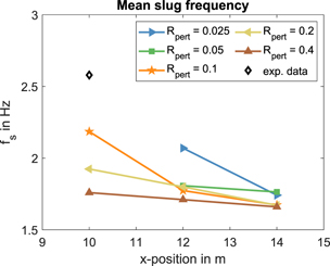
Figure 11. Mean slug frequency calculated from the simulated liquid level time series at different x-positions for different perturbation amplitudes (colored lines) and corresponding experimental data at x = 10 m (black diamonds).
Download figure:
Standard image High-resolution imageFigure 12 shows histograms of the inverse slug unit time,  , for three perturbation amplitudes (Rpert = 0.1, Rpert = 0.2, and Rpert = 0.4) in comparison with experimental data. Note that, for the two lowest perturbation amplitudes, Rpert = 0.025 and Rpert = 0.05, slug flow is just evolving and, therefore, it does not make sense to consider histograms due to the low number of slugs observed at this stage. In all the pictures in figure 12, the blue scale on the left indicates how often a certain time difference between two consecutive slugs occurs. Thus, the sum over all counts gives the total number of slugs observed in the considered time interval. Since the experimental liquid level time series are obtained from a time interval of more than 2 min, the counts in figure 12(d) are much higher than for the simulation data (a)–(c), where only 50 s have been considered. Therefore, we also plotted the fitted probability density functions (pdfs) (red lines in figure 12), which are independent of the total number of counts. Their shapes show good agreement between experiment and simulation, especially for the case Rpert = 0.1.

Figure 12. Histograms and fitted pdf of the inverse slug unit time,  , for simulations with three different perturbation amplitudes, (a) Rpert = 0.1, (b) Rpert = 0.2, (c) Rpert = 0.4, and (d) corresponding experimental data.
Download figure:
Standard image High-resolution image4. Conclusions
When multiphase flows are modeled, complex geometrical and operational features of the experiments, such as the phase mixing section, are often not resolved in the numerical simulation. Rather simplified boundary conditions are used, which usually impose less turbulence into the system than present in reality. Hence, inlet perturbations can be used in the numerical simulation in order to induce instabilities at the interface leading to a more natural behavior.
In this paper, a perturbation that randomly disturbs the secondary components of the velocity vector at the inlet is proposed in order to enhance the formation of slugs in the pipe. It is shown that, the higher the perturbation amplitude, the earlier the slugs occur. On the other hand, sufficiently far away from the inlet, the flow pattern shows the same dynamics for all the different perturbation amplitudes indicating that no specific frequency is imposed by the prescribed perturbation in contrast to the outcome of simulations with sinusoidal perturbations that have been used previously.
Altogether, our simulation results clearly show that horizontal slug flow develops through different stages. Near the inlet, a stratified or wavy flow regime is monitored followed by a zone in which slug precursors are developing. Further downstream in the pipe, larger slugs can be observed and the flow enters into a saturated stage, where the dominant frequencies of the interface dynamics are not changing anymore. However, this saturated stage cannot be equated with stable or fully developed slug flow, where not only the interface dynamics, but also other mean parameters of the slugs (such as the mean slug length) do not change anymore. This stage is expected to be observed even further downstream in the pipe. In order to ensure comparable measurement conditions for a measurement device installed at a fixed location in the pipe, it is important to specify in which of the identified zones the measurement is performed. Our simulation results can help to classify different stages of slug flow that can be observed during the measurement process.
We like to emphasize that the simulations presented here reveal that slug flow is more complex than single phase flow, where usually measurement conditions become more favorable further downstream since the perturbation of the flow typically decays and an ideal symmetric profile is eventually approached, see, e.g., [2]. For multiphase flow, on the other hand, the flow does not become stationary with sufficient distance from the inlet. Even fully developed flow patterns are still transient and the distribution of the different phases in the pipe changes permanently. In order to ensure comparable measurement conditions or to facilitate intercomparisons between different laboratories or facilities, it has to be analyzed in which qualitative regime the flow is monitored. The observed flow pattern at a fixed position in the pipe is strongly dependent on the boundary conditions at the inlet. In practice, these conditions are not uniform, but specific for each laboratory, leading to different levels of mixing between the phases near the inlet. In our numerical simulation, this is modeled by considering and comparing different perturbation amplitudes.
Our simulation provides a first systematic guideline and insight how inlet perturbations affect the actual location of the evolving flow regimes in the pipe. Future work based on the analysis of measured and simulated multiphase flows shall address the correlations of the flow pattern (transient stratified, growing slug or saturated slug flow) with registered uncertainties of multiphase flow measurement.
Acknowledgments
This work was supported through the Joint Research Project Multiphase flow reference metrology. This project has received funding from the EMPIR programme co-financed by the Participating States and from the European Union's Horizon 2020 research and innovation programme. The authors would like to thank Terri Leonard and Marc MacDonald from TÜV SÜD NEL, who provided the experimental video observations.
Appendix A.: On the influence of sinusoidal inlet perturbations on the evolution of slugs
In this section, the influence of sinusoidal inlet perturbations on the development of slug flow in horizontal pipes is investigated. This idea goes back to Frank, who prescribed a sinusoidally varying liquid level at the inlet of the pipe in order to enhance the development of slugs [22]. We use the same set-up as in [22] so that our results can directly be compared with the results in this paper as well as with corresponding experimental data from [45]. Hence, we consider two-phase air-water flow through a horizontal pipe with an inner diameter of D = 0.054 m and a length of L = 8 m.
The distribution of both phases in the computational domain was initialized as depicted in figure A1. Below the prescribed liquid level (blue line in figure A1), the liquid volume fraction was set to one, above it was set to zero. For t = 0, vertical position of the interface, hl, was defined as

Furthermore, a transient liquid level was prescribed as boundary condition on the inlet:

where Ui = 2 m s−1 is the liquid/gas velocity prescribed on the inlet. Hence, this boundary condition corresponds to an agitation frequency of fa = 1 Hz. In order to investigate the influence of the agitation frequency, fa, on the slug frequency further downstream in the pipe, we varied this parameter between 0.5 Hz and 2 Hz in our simulations.
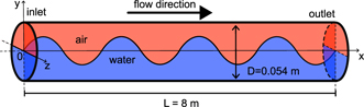
Figure A1. Illustration of the initial condition used for the simulation of the air–water slug flow test case (not to scale).
Download figure:
Standard image High-resolution imageThe multiphase flow simulations were performed using the commercial CFD solver ANSYS Fluent [46]. The interface between the two phases was modeled by the VOF method [35]. The k-ω-SST model [37] was chosen as turbulence model within an unsteady RANS approach. A detailed description of the numerical discretization schemes can be found in [47]. We validated our CFD model by comparing our results for fa = 1 Hz with the data provided in [22] as well as with experimental data from [45], see table A1.
Table A1. Comparison between experimental data from [45], simulation results from [22], and our simulation.
| Slug period | Slug velocity | |
|---|---|---|
| Exp. by [45] | ca. 1.8 m | ca. 2.7 m s−1 |
| Sim. by [22] | ca. 2.7 m | (2.7–3.1) m s−1 |
| Our simulation | ca. 2.7 m | (2.7–2.8) m s−1 |
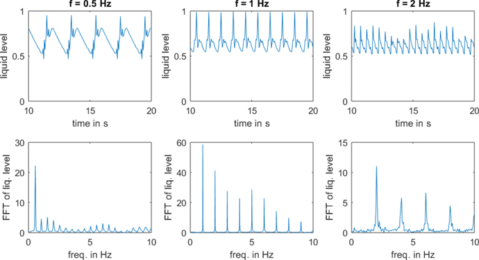
In the following, we shortly summarize our results for different agitation frequencies, fa. Figure A2 shows the liquid level time series for a time interval of 10 s as well as the corresponding FFT spectra for three different agitation frequencies, fa = 0.5 Hz, fa = 1 Hz, and fa = 2 Hz. One observes periodic flow in all cases. In the pictures in the top of figure A2, one can count five slugs for the agitation frequency of 0.5 Hz, ten slugs for 1 Hz, and 20 slugs for 2 Hz. This shows that the prescribed agitation frequency is reflected in the slug frequency. This observation is confirmed by a frequency analysis, see pictures in the bottom of figure A2. The peaks in the FFT spectrum of the liquid level time series occur at exactly the prescribed agitation frequencies. In all cases, the spectra show only the agitation frequency fa and its harmonics.
Figure A2. Top row: liquid level versus time for three different agitation frequencies. Bottom row: corresponding FFT of the liquid level for the same cases.
Download figure:
Standard image High-resolution image