


Abstract
When flow meters are installed in disturbed flow conditions caused by pipe configurations such as junctions or elbows, significant measurement errors can occur. With existing knowledge of the flow conditions, those errors can be corrected using suitable calibration factors. This paper presents a surrogate model based on computational fluid dynamics simulation results that can predict velocity profiles downstream of single and double elbows in- and out-of-plane. The simulated flow profiles are decomposed into a fully-developed and a disturbed part, which allows changing the Reynolds number and roughness of the pipe wall without performing additional simulations. Furthermore, proper orthogonal decomposition and interpolation using piecewise linear splines enables the real-time evaluation of the model for a wide range of curvature radii and distances between the elbows. By incorporating a measurement principle, calibration factors for different flow meter designs can be predicted. The model is validated on the example of an ultrasonic flow meter by comparison with measurement data obtained from a clamp-on flow meter.
Export citation and abstract BibTeX RIS

Original content from this work may be used under the terms of the Creative Commons Attribution 4.0 license. Any further distribution of this work must maintain attribution to the author(s) and the title of the work, journal citation and DOI.
1. Introduction
Flow meters are usually provided with calibration values that rely on the assumption of a fully developed symmetrical velocity distribution. Such ideal flow conditions require a long, straight pipe section to develop. In practical applications, however, the presence of elbow configurations, junctions, and other installations cause disturbed flow conditions with asymmetric velocity distributions and secondary flow motions. This can create significant measurement errors leading to incorrect billing and inefficiencies in industrial processes. With existing knowledge of the local flow conditions, the meter error due to flow disturbances can be corrected for any particular measurement procedure and design. This can be accomplished by means of fluid mechanical calibration factors, which can be determined experimentally through measurements with the meter itself or calculated from the velocity distributions provided by visualizing techniques such as laser Doppler anemometry and particle image velocimetry (PIV). Alternatively, calibration factors can be determined in flow simulations using computational fluid dynamics (CFD).
While measurements can provide highly accurate results, they are often costly and time-consuming and thus, limited to specific geometries only. This presents a problem as in reality there is a wide range of potential elbow configurations, each resulting in a different flow development downstream. More specifically, the standards for butt-welding pipe fittings EN 10 253-2/-4:2017 [5, 6] distinguish between 2D, 3D, and 5D models with curvature radii of around 1.0, 1.5 and 2.5 pipe diameters. Additionally, custom-built elbows with curvature radii ranging from 0.5 to 5 pipe diameters or even higher are used. Double elbow configurations may also vary in the orientation and distance between the two bends. In comparison to experiments, CFD simulations can be conducted for a broad variety of configurations. On the downside, their accuracy is dependent on the validity of the underlying model assumptions and on how accurately the geometry, boundary conditions, etc can be reproduced in the numerical model. Simulations with the industry standard RANS (Reynolds-averaged Navier–Stokes) can be carried out in relatively short time but are known to be inaccurate in complex flows that include swirl or flow separation. Transient, scale-resolving models on the other hand are too time-consuming to be practical for a large number of parameters and relevant Reynolds numbers in industrial applications.
Various studies have been conducted to assess the effects of elbow configurations on the downstream flow development, especially with regard to flow meter performance. As for numerical studies, the flow development downstream of both single and double elbows out-of-plane has been investigated with regard to varying inflow conditions (Weissenbrunner et al [34, 35]), Reynolds numbers (Martins [16], Holm et al [12]), circumferential and axial mounting positions of ultrasonic flow meters and the sensitivity of the associated simulations (Martins et al [17, 18]), comparison with measured data from laser Doppler velocimeters (Moniz Pereira [22]) and ultrasonic velocity profilers (Tsuzuki et al [31]). Other numerical studies have examined the flow adaptivity of ultrasonic flow meters downstream of a SE (Zheng et al [41]), the effects of pipe wall roughness downstream of a double elbow out-of-plane (Morrison and Tung [23]) and the flow behind 180∘ elbows with different curvature radii (Bilde et al [1]). Zheng et al [40] present simulations that are able to infer the effect of the disturbed flow past single and double elbow geometries on the sound pressure propagation. As for experimental studies, LDV measurements downstream of both single and double elbows out-of-plane have been performed to analyze the disturbed velocity profiles (Wendt et al [37]), and, to investigate the effects on ultrasonic and electromagnetic flow meters (Turiso et al [32], Straka et al [28], Halttungen [10]) as well as on turbine meters, orifice flow meters and tube bundles (Mattingly and Yeh [19–21], Kelner [14]). Furthermore, PIV measurements have been carried out downstream of a double elbow out-of-plane in conjunction with flow conditioners (Xiong et al [39]), with focus on the spatio-temporal flow structures downstream of a SE (Hellstroem et al [11]) and with emphasis on the decay of Dean vortices downstream of a SE (Kalpakli and Örlü [13]). Although research activity is very high, the majority of scientific investigations have been constrained to examining only one or a few distinct elbow geometries. However, comprehensive models to efficiently predict calibration factors in a broad range of geometric parameters do not yet exist.
The aim of this study is to develop a tool capable of determining the flow conditions downstream of practically relevant elbow configurations. This is realized by means of a surrogate model constructed from a total of 263 RANS simulations. Its scope covers single and double elbow configurations both in- and out-of-plane with curvature radii and distances between the elbows ranging from 0.5 to 10 and 0 to 5.5 pipe diameters, respectively. Furthermore, it is possible to modify the Reynolds number and pipe wall roughness. By modeling the measurement principle, calibration factors for arbitrary meter designs can be calculated.
The paper is structured as follows: section 2 covers the numerical setup for the CFD simulations and a selection of simulation results to illustrate the diverse flow phenomena downstream of different elbow geometries. The construction of the surrogate model is described in section 3. This includes decomposing the velocity fields predicted in the CFD simulations into fully developed and disturbed parts as well as a proper orthogonal decomposition (POD) analysis to reduce the amount of data. Finally, the utilization of the surrogate model as a virtual flow meter is demonstrated on the example of an ultrasonic flow meter in section 4. This includes a validation with calibration factors obtained from measurements with clamp-on flow meters installed downstream of a single and a double elbow out-of-plane.
2. Simulation setup
In this section, the numerical setup of the CFD simulations is described. This includes the geometry, flow conditions, solver settings and a grid study. Additionally, a selection of flow profiles downstream of the elbow configurations is shown to demonstrate the dynamics in the parameter space.
2.1. Geometry
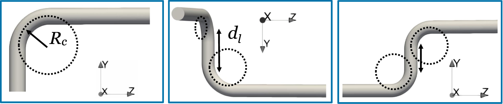
Three different 90∘ elbow configurations of circular pipes with a pipe diameter of D = 0.1 m are studied: a single elbow (SE), a double elbow out-of-plane (DE) and a double S-elbow (DSE), compare figure 1. The geometrical degrees of freedom are the curvature radius  (for all cases) and the distance between the two elbows
  (for the geometries with two elbows DE and DSE). Multiple geometries with different parameter realizations are generated. For the SE case, the curvature radius
  is sampled between
  and
and  in
in  steps. Note that
  is chosen to be
  higher than the theoretical minimum (
 ) to avoid a sharp edge, which would lead to grid elements with low quality. As the dynamics are expected to be higher at lower values of
  , the sample positions are distributed according to
For the other two cases, values of  and
and  are chosen. The distance between the two elbows
 ![$d_l \in [d_\textrm {l.min},d_\textrm {l.max}]$](https://content.cld.iop.org/journals/0026-1394/60/5/054002/revision4/metace7d6ieqn14.gif) is distributed according to
is distributed according to
where the minimum and maximum distances are  and
and  , respectively. The number of parameter values is
  .
.
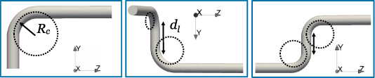
Figure 1. The studied geometries with the free parameters  (curvature radius) and dl
(distance between the elbows), from left to right: single 90∘ elbow (SE), double elbow out-of-plane (DE) and double S-elbow (DSE).
(curvature radius) and dl
(distance between the elbows), from left to right: single 90∘ elbow (SE), double elbow out-of-plane (DE) and double S-elbow (DSE).
Download figure:
Standard image High-resolution imageAltogether, a total of 263 geometries are processed. The geometries and meshes are generated automatically using the BlockMesh implementation from [24]. In the computational domain, the length from the inlet to the entry of the upstream elbow is  , while the straight pipe section between the exit of the downstream elbow and the outlet has a length of
  .
.
2.2. Flow conditions
The flow conditions in the simulations are selected in conformity with the measurement setup described in Straka et al [28, 29]. The water temperature is 30 ∘C, which results in a kinematic viscosity of  m2 s−1. Furthermore, the flow rate is 11.32 m3 h−1, which corresponds to a volumetric velocity of
  m s−1. This results in a diameter-based Reynolds number of
  and a friction Reynolds number of
  for a smooth pipe. At the inlet, a fully developed velocity profile and turbulent viscosity taken from a precursor simulation of a straight pipe is prescribed. At the outlet zero pressure, and zero velocity at the pipe walls, are prescribed.
2.3. Solver settings
In order to perform a CFD simulation, it is necessary to solve mathematical equations that describe the behavior of the fluid. The fluid motion of water can be described by the incompressible Navier–Stokes equations. As the resolution of all turbulent fluctuations is computationally too expensive, additional equations can be included to model the effects of turbulence. There are different types of turbulence models for transient simulations such as large eddy simulation (LES) or detached eddy simulation (DES), see, e.g. Ferzinger and Peric [7], Wilcox [38]. These models resolve large turbulent flow structures and model the effect of the smallest turbulent scales, yet they are still too computationally expensive, especially for high Reynolds numbers. In this study a large number of simulations needs to be performed at a comparatively high Reynolds number. Therefore, RANS models are employed, which are less computationally expensive by several orders of magnitude. RANS models rely on a time-averaged version of the Navier–Stokes equations and additional transport equations to calculate an artificial local eddy viscosity that accounts for all turbulent fluctuations. Among the RANS type models, the most common approaches are the k-ε, k-ω and SST model. As of today, these models are still the industry standard. In this study, the Spalart–Allmaras turbulence model [26] is used, which consists of one partial differential equation for calculating the eddy viscosity  . Although being less computationally expensive, it has been demonstrated to be equally or even more precise compared to other RANS models in pipe flow applications, see Straka et al [29].
Second order discretization schemes are chosen, for divergence of the velocity bounded Gauss linear and bounded Gauss linearUpwind grad(U) for the divergence of the turbulent viscosity. Moreover, Gauss linear and Gauss linear corrected are used for the gradient and Laplacian schemes, respectively. For the DE and DSE the solver OpenFOAM version 1812 is used, whereas for the SE, RapidCFD is used. Both solvers are based on the finite volume method. RapidCFD is a fork of OpenFOAM (version 2.3) operating on GPU, which produces similar results for the Spalart–Allmaras turbulence model, see Ekat et al [4].
2.4. Grid study
A grid-independence study is conducted to ensure the accuracy of the numerical solution of the mathematical equations. Block-structured hexahedral O-grids are created using BlockMesh with increasing grid densities. The study is conducted for a DE with  and
and  . Five grids are created, each with an inlet length of
  between the inlet and the elbow entrance, and an outlet length of
  downstream of the last elbow. The coarsest grid, labeled G0, contains 160 000 elements. Subsequent grids G1 and G3 have twice and quadruple the number of grid cells in all three dimensions compared to G0. Grid G2 is created by refining G1 slightly, and the finest grid, G4, is generated by moderately refining G3. The grid parameters are summarized in table 1. A quarter of the pipe cross section for G0, G1, G3 and G4 as well as the full cross section of G2 are presented in figure 2.
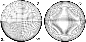
Figure 2. Left: a quarter cross section of the computational grids  , and G4. Right: a cross section of the grid G2 chosen for the CFD simulations.
Download figure:
Standard image High-resolution imageTable 1. The parameters of the computational grids used for the simulations in the grid study, where  is the number of grid elements in millions,
  the dimensionless distance of the first grid cell to the pipe wall (mean, minimum and maximum value over the whole fluid domain), Nxy
the number of discretization points in the x and y direction in the inner core of the O-grid, No
the number of radial elements of the outer ring and Nz
the number of grid elements in flow direction per diameter D.
the dimensionless distance of the first grid cell to the pipe wall (mean, minimum and maximum value over the whole fluid domain), Nxy
the number of discretization points in the x and y direction in the inner core of the O-grid, No
the number of radial elements of the outer ring and Nz
the number of grid elements in flow direction per diameter D.
| Grid Name |

|
 (min, max) (min, max) | Nxy | No | Nz per D |
|---|---|---|---|---|---|
| G4 | 35 | 0.2 (0.03, 0.3) | 60 | 75 | 24 |
| G3 | 9 | 0.3 (0.04, 0.5) | 40 | 50 | 16 |
| G2 | 2 | 0.5 (0.08, 1) | 26 | 32 | 10 |
| G1 | 1 | 0.8 (0.1, 1.3) | 20 | 25 | 8 |
| G0 | 0.1 | 2 (0.5, 4) | 10 | 12 | 4 |
To compare the performance of the grids, the magnitude of the difference between the velocity vectors of the results with each grid
u
i
and the finest grid  is calculated according to
  . After that, the L2-norm over the cross sections Ω is evaluated at multiple downstream positions z:
Here, A is the area of the cross section Ω. All velocities  are normalized with the bulk velocity uvol
, so that
are normalized with the bulk velocity uvol
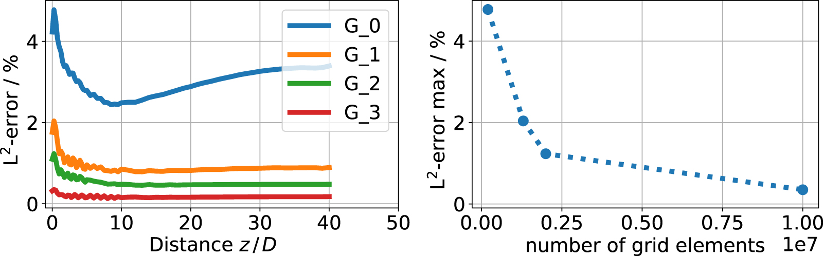
, so that  . The result of each grid is interpolated onto the cell centers of the coarsest grid G0. All integrals are calculated using piecewise linear shape functions on a Delaunay triangulation of the x–y coordinates. It can be observed that for all grids the highest deviations appear near the elbow exit and decline with further distance, compare figure 3 (left). In figure 3 (right), the maximum of
  over all evaluated cross sections for each grid,
  , is shown over the number of grid elements. As a compromise between accuracy and efficiency, the parameters of G2 are chosen for the simulations of the elbows with the geometry variation. Other than in the grid study, the length of the straight pipe downstream the elbow is extended to
  . This leads to a number of grid elements between
  and
and  .
.
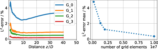
Figure 3. The L2-error  from equation (3) of the resulting velocity profiles calculated with the grids
  compared to the finest grid G4. Left: over the distance z to the elbow exit, right: the maximum error of each grid over the number of grid elements.
Download figure:
Standard image High-resolution image2.5. Results
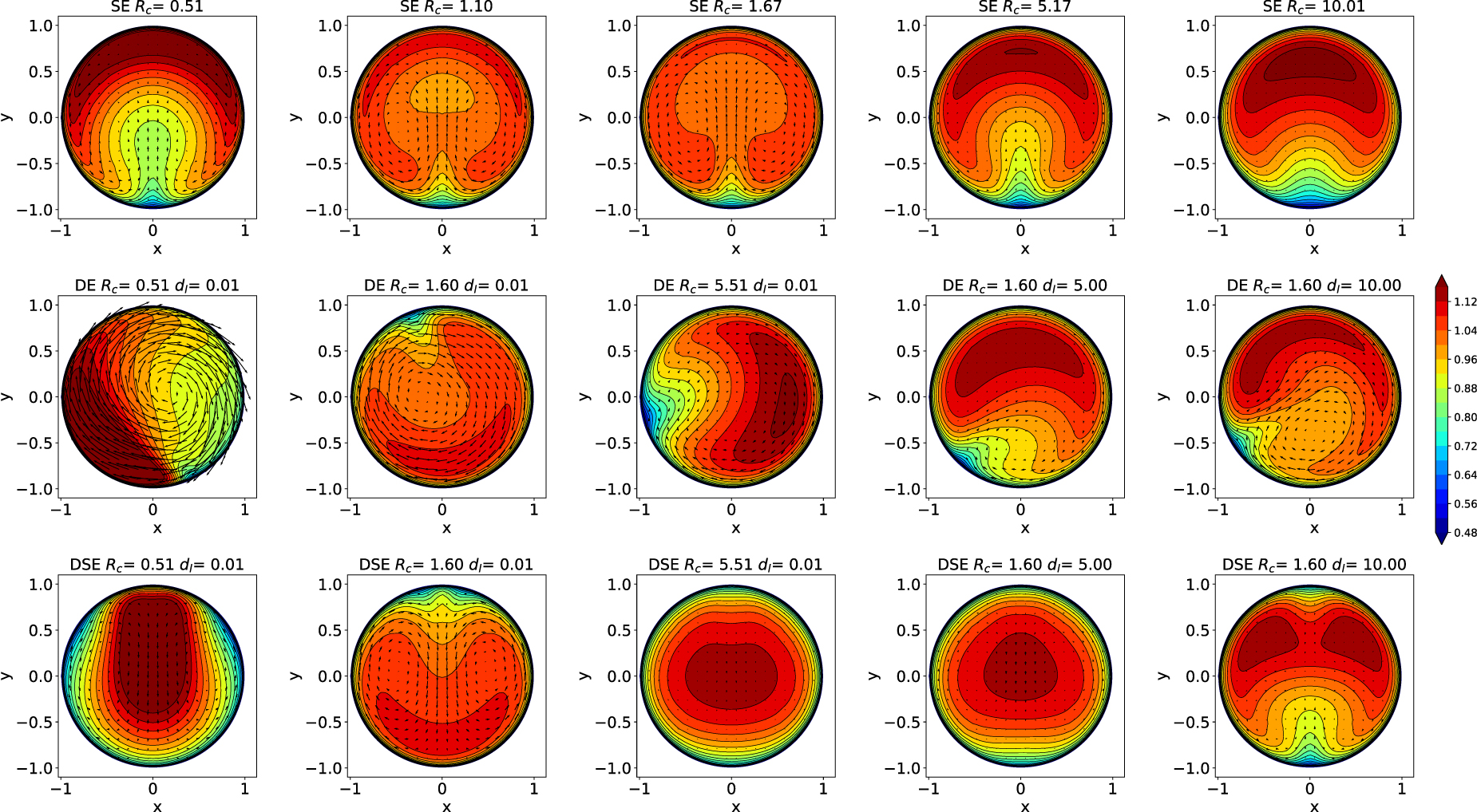
In general, the flow downstream of all geometries is highly disturbed which manifests in asymmetric axial velocity profiles and enhanced secondary flow motions. A brief overview of the resulting velocity profiles at  with different values of
  and
and  is shown in figure 4. For the SE (top row), the typical sickle-shaped axial velocity profile can be observed, where the conformation of the shape differs with different values of
  . The secondary flow motions, which are represented by arrows, show two counter-rotating swirls. Downstream of the DE (center row) the profile is also sickle-shaped but, in contrast to the SE, it is rotating clockwise due to the centered single swirl. The variation of shapes downstream of the DSE (bottom row) is more divers. The position of the highest axial velocities varies between the upper, lower, and center part of the pipe cross section. The secondary flow motions build two counter-rotating swirls, similar to the SE but in opposite direction. With higher values of
  and
and  , the strength of the swirl gets weaker for the depicted velocity profiles. Note that the plots represent only a small part of the results, but illustrate the complexity of the dynamics in the parameter space.

Figure 4. Contour plots of the axial velocity profiles uz
at  downstream of the SE (first row), DE (second row), and DSE (third row) with different values of
  and
and  . The arrows denote the secondary flow motions
  .
.
Download figure:
Standard image High-resolution image3. Construction of a surrogate model
In this section the construction of a surrogate model based on the simulation results in section 2 is described. It allows the prediction of the time-averaged velocity fields for arbitrary positions up to  downstream of the SE, DE or DSE for any curvature radius
 ![$R_\textrm c \in [0.51, 5.51] \, D$](https://content.cld.iop.org/journals/0026-1394/60/5/054002/revision4/metace7d6ieqn56.gif) , any in-between distance
, any in-between distance ![$d_\textrm l \in [0.01,10.01] \, D$](https://content.cld.iop.org/journals/0026-1394/60/5/054002/revision4/metace7d6ieqn57.gif) , and any Reynolds number
, and any Reynolds number ![$Re \in [5,50]\cdot 10^4$](https://content.cld.iop.org/journals/0026-1394/60/5/054002/revision4/metace7d6ieqn58.gif) . The following steps are performed to construct the surrogate model: At first, the velocity data is sampled from the simulation results and the velocity profiles are decomposed into a fully developed and a disturbed part. Then, a POD is performed to reduce the amount of data. Finally, an interpolation is proposed that can be used to predict velocity profiles throughout the specified range of geometrical parameters.
. The following steps are performed to construct the surrogate model: At first, the velocity data is sampled from the simulation results and the velocity profiles are decomposed into a fully developed and a disturbed part. Then, a POD is performed to reduce the amount of data. Finally, an interpolation is proposed that can be used to predict velocity profiles throughout the specified range of geometrical parameters.
3.1. Data sampling
For each simulation, the velocity field at each cross section is sampled in cylindrical coordinates  . Whereas the angular positions are chosen uniformly, the radial positions are chosen to be more dense at the wall according to
Similarly, the downstream positions z are sampled with a higher density close to the elbow exit with
The corresponding number of sampled data points are summarized in table 2.
Table 2. The number of data points sampled from the simulation results with regard to the velocity components (Nu
), curvature radii ( ), in-between distances (
 ), downstream positions (Nz
), radial positions (Nr
), angular positions (Nϕ
), and the overall data points in millions (
), downstream positions (Nz
), radial positions (Nr
), angular positions (Nϕ
), and the overall data points in millions ( ).
).
| Case | Nu |

|

| Nz | Nr | Nϕ |
 /106 /106
|
|---|---|---|---|---|---|---|---|
| SE | 3 | 21 | — | 101 | 41 | 81 | 21 |
| DE | 3 | 11 | 11 | 200 | 41 | 81 | 241 |
| DSE | 3 | 11 | 11 | 151 | 41 | 81 | 182 |
3.2. Decomposition of the velocity profile
The axial velocity profile uz
can be decomposed into a fully developed part  and a disturbed part
  according to

This decomposition offers the benefit of utilizing an analytical approach for the fully developed part of the profile. Consequently, varying the Reynolds number (Re) or sand grain roughness ( ) can be achieved without the requirement of performing a new simulation. By replacing
  with modified parameters of Re and
  in equation (6), a new profile uz
is created. In figure 5, the decomposition of the velocity profile is illustrated on the example of a vertical line at
in equation (6), a new profile uz
is created. In figure 5, the decomposition of the velocity profile is illustrated on the example of a vertical line at  downstream of the SE with
  D with original parameters
  and with modified parameters
  and
and  . As an important property, this decomposition conserves the flow rate. This approach implies that
  is independent of the Reynolds number and the pipe wall roughness. A similar approach can be found in Gersten and Papenfuss [9]. This approach is reasonable for moderately high Reynolds numbers (
 ). Note that for the decomposition,
  is taken from a simulation of a long straight pipe, whereas for the reconstruction,
  is calculated with the semi-analytical formulation from Gersten [8]. This alteration of the profile is insignificant in regions of strong disturbance (close to the elbows), but eliminates systematic errors which are inherent in simulation results of fully developed pipe flow. Even though the theoretical profile is also an approximation, it is in better agreement with measurement data than simulation results with RANS models, see, e.g. Tawackolian [30].

Figure 5. Decomposition of the axial velocity profile along a vertical line  at
at  downstream of the SE with
  D; left: uz
, center:
D; left: uz
, center:  and right:
  , compare equation (6). The continuous blue line represents the original simulation result with
  and a smooth pipe wall with sand-grain wall roughness of
  , the dashed orange line represents a predicted solution with
  and
and  , and the dotted green line represents the solution with
  and
and  .
.
Download figure:
Standard image High-resolution image3.3. POD
To reduce the amount of data, the velocity profiles  can be further decomposed with the method of POD. While POD is extensively used in the analysis of temporal fluctuations in fluid dynamics, see, e.g. Hellstroem et al [11] or Sieber et al [25], it can also be used to reduce the dimensions of a data set, e.g. Brunton and Kutz [2]. To accomplish that, the data matrices need to be reorganized such that the data matrix of each of the
  cross sections is flattened as a row vector
  . These vectors are treated as snapshots, similar to transient data, and are stored in the rows of the matrix
 ![$\boldsymbol{B} = \left[ \boldsymbol{b_1} , \boldsymbol{b_2}, {\ldots} \boldsymbol{b_{N_s}}\right]$](https://content.cld.iop.org/journals/0026-1394/60/5/054002/revision4/metace7d6ieqn94.gif) . Then, the mean vector
. Then, the mean vector  over all rows
  is subtracted to receive the matrix

and its covariance matrix
Its eigenvalues λ and modes Φ are calculated by an eigendecomposition

The modes are sorted in descending order of their corresponding eigenvalues, so that the first modes contain most of the energy. The coefficient matrix
A
can be determined by the scalar product of the data matrix  and the modes Φ according to

The original data matrix B can be approximately reconstructed with
where  and
and  are the ith column of
A
and Φ, respectively, and
are the ith column of
A
and Φ, respectively, and  is the number of modes used for the reconstruction. Furthermore,
  is the number of data in one cross section and
  the number of sampled planes ('snapshots'). Instead of storing the data matrix
  , only the mean data vector
  , the coefficient matrix
  and the modes
  need to be stored. If the number of used modes
  is small enough, the amount of data is reduced, since
  if
if  . In this paper, the POD is not just done for one set of parameters but for all parameter combinations and cases together. Hence, the data matrix
B
is constructed by stacking the velocity profiles of all cases, resulting in
. In this paper, the POD is not just done for one set of parameters but for all parameter combinations and cases together. Hence, the data matrix
B
is constructed by stacking the velocity profiles of all cases, resulting in  .
.
Contour plots of  and vector plots of the secondary flow motions ux
and uy
of the mean profile
and vector plots of the secondary flow motions ux
and uy
of the mean profile  and the first eight modes are shown in figure 6. The typical sickle-shaped asymmetry of the velocity profiles can be observed, especially in the mean profile. Also, different flow structures such as single swirl (mean profile and mode 2), typically for the DE case, as well as pairs of counter-rotating swirls, so called Dean vortices [15], (mode 4 and mode 7) can be observed.

Figure 6. Contour plots of the axial velocity components  and vector plots of the secondary flow motions ux
and uy
of the mean profile
and vector plots of the secondary flow motions ux
and uy
of the mean profile  (top left) and the first eight modes of the POD calculation
  (ascending from top to bottom and left to right).
Download figure:
Standard image High-resolution imageTo determine the number of modes that have to be considered, the velocity field
u
is reconstructed for an increasing number of modes. The L2-error  from equation (3) is calculated, with
  being the magnitude of the difference of the approximated velocity field
  (
( ) reconstructed with i modes and
u
(
) reconstructed with i modes and
u
( ) the original simulation data. Both the mean and maximum of
  over the whole data set for each case and over the number of used modes
  is shown in figure 7. It can be observed that the errors decline with an increasing number of modes, and that the mean errors are smaller than the maximum errors by a factor of about 10. A total of
  modes are chosen as a good balance between accuracy and efficiency. As a result, the maximum error
  is 0.35% and the mean error of
  is smaller than 0.025%. This means that the data can be reduced by a factor of 20. In other words, it is possible to reconstruct the entire data with an error of less than 0.4% by storing 5% of the data.

Figure 7. The mean (left) and maximum (right) L2-error  of the reconstructed flow field from the POD and the simulated flow field according to equation (3) in percentage over the number of used modes
  .
.
Download figure:
Standard image High-resolution image3.4. Interpolation of the POD coefficients
Predicting the velocity distribution within the three dimensional (physical) space and for arbitrary values in the space of geometry parameters requires an interpolation of the POD coefficients. In the x–y (or r–ϕ) space, the interpolation can be performed within each of the POD modes. To obtain the velocity profile at any spatial position z, curvature radius  and in-between distance
  , the POD coefficients
  of each mode (compare equation (11)) need to be interpolated. The high dynamics of
  for low parameter values can be observed in the contour plots of figure 8. To perform the interpolation,
  must be reshaped to restore its original dimensionality
  . This corresponds to a 2D interpolation for the SE and 3D interpolation for the two other cases. Here, a tensor-product spline interpolation implemented in the python package scipy.interpolate called RegularGridInterpolator is used, see Weiser and Zarantonello [33]. This method enables an interpolation on n-dimensional rectangular shaped grids.
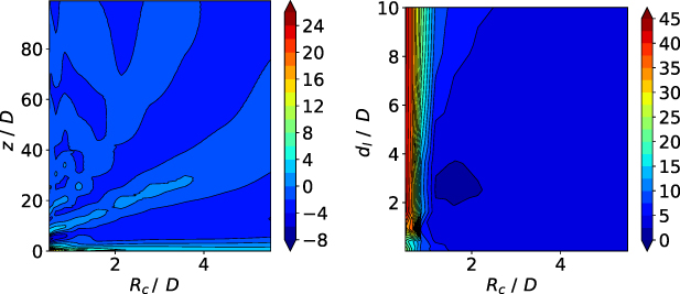
Figure 8. Contour plots of the POD coefficients of the first mode for the DE for two different parameter sets:  (left) and
  (right).
Download figure:
Standard image High-resolution imageTo check the accuracy of the interpolation, a so called cross validation procedure is performed, in which one of the sample positions in  is left out. To maintain the rectangular grid structure of the samples, a whole slice (row/column in 2D) of values is removed. Afterwards, the interpolation is performed with the remaining samples and the velocities
  are calculated for the previously eliminated parameters. The difference to the original simulation results is calculated as
  and assessed by means of the L2-error
  , compare equation (3). The procedure is repeated consecutively for each value of the sampled parameters except for the upper and lower parameter values, which are always included. Interpolations with spline functions of polynomial degree p = 1 (linear), p = 3 (cubic) and p = 5 (quintic) are compared in figure 9(a), where the mean L2-error over all Rc
and dl
,
, compare equation (3). The procedure is repeated consecutively for each value of the sampled parameters except for the upper and lower parameter values, which are always included. Interpolations with spline functions of polynomial degree p = 1 (linear), p = 3 (cubic) and p = 5 (quintic) are compared in figure 9(a), where the mean L2-error over all Rc
and dl
,  , is shown for the interpolation at each downstream distance z. For the linear interpolation, errors with a maximum of 2% occur near
  . For the higher polynomial spline interpolations, the errors are distinctively lower.
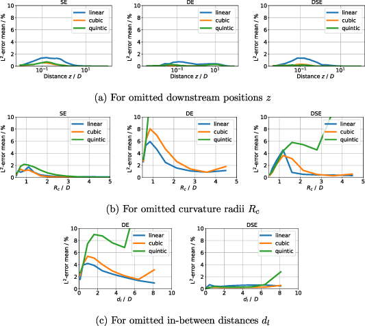
Figure 9. Mean L2-errors in percentage with regard to the magnitude of the differences between the reconstructed velocities using interpolated and exact POD coefficients, for each parameter and case.
Download figure:
Standard image High-resolution imageFigure 9(b) shows the mean of  over all z and
  at each curvature radius
  for the SE, DE and DSE cases. With linear interpolation, the values rise up to 6% at
  , whereas the errors of the cubic spline polynomials are in general slightly higher. Quintic interpolation produces significantly high errors for both the DE and DSE cases.
The mean of  over all z and
  is shown at each in-between distance
  for the DE and DSE in figure 9(c). Errors with piecewise linear interpolation show a maximum of 4% at
  for the DE and below 1% for the DSE. For the DE, the cubic interpolation errors are higher than the linear, and the quintic ones are beyond 10% for
  .
.
In conclusion, the cross validation study is useful to identify parameter regions worth of refining, as well as for comparing the performance of different interpolation methods. In certain cases, the failure of spline interpolation with higher order polynomials can be attributed to its oscillating nature, which has a tendency to over- and undershoot, especially if the interpolation points are not perfectly smooth. Moreover, the steep gradients concentrated at low values of  , z and
  as well as the unsteadiness of the sampled data are challenging for any interpolation method. The high interpolation errors are located at positions in proximity to the elbow exit
  and small values of
  , where recirculating flow is present. Overall, the comparison between the spline interpolations with different polynomial degrees yields that piecewise linear interpolation provides the most reliable method with mean errors of less than 6%.
4. Flow meter evaluation
The calculated velocity profiles can be used to predict errors, calibration factors or uncertainties of specific types of flow meters. Especially non intrusive measurement principles such as ultrasonic and electro-magnetic flow meters can be modeled in post processing. In the following, the procedure is shown on the example of an ultrasonic flow meter. Calibration factors for this type of flow meter are modeled and compared with measurement data of an ultrasonic clamp-on flow meter.
4.1. Model of an ultrasonic flow meter
The most common type of ultrasonic flow meter uses the time-of-flight principle. A transducer (A) induces a sonic wave into the pipe, which is detected by another transducer (B) installed further downstream. The time between sending and receiving the signal is measured. This procedure is repeated, whereas the downstream transducer is sending and the upstream transducer is receiving. Since the fluid flow is carrying the sound waves, the measured time is proportional to the mean flow velocity along its traveled path  . The transducers can be aligned to directly send the sonic waves to each other or by using one or more reflections at the pipe wall. A common configuration with one reflection is the so-called V-path configuration, compare figure 10. If the velocities in the pipe are known, the measurement value of an ultrasonic flow meter can be predicted by evaluating the integral
Here,  denotes the length of the ultrasonic path from one transducer to the other,
e
i
is the direction vector parallel to the ultrasonic beam, and
denotes the length of the ultrasonic path from one transducer to the other,
e
i
is the direction vector parallel to the ultrasonic beam, and  the mean axial share of the direction vectors
e
i
.
the mean axial share of the direction vectors
e
i
.

Figure 10. The ultrasonic V-path configuration.
Download figure:
Standard image High-resolution imageTo determine the volume flow Q of the fluid inside the pipe, the measured path velocity  must be multiplied by the area of the pipe cross section A and a calibration factor k that assigns the mean velocity over the path to a mean velocity over the pipe cross section:

The calibration factor k is dependent on the velocity profile. For fully developed flow conditions, it only depends on the Reynolds number Re and the wall roughness  as
as  only depends on r, Re, and
  (cp. equation (6)):
For disturbed flow conditions, an additional calibration factor
can be introduced. The fluid-specific calibration factor is then calculated as  . In a long straight pipe, kd
is approaching a value of one, as
. In a long straight pipe, kd
is approaching a value of one, as  is converging to zero.
4.2. Interpolation of the flow meter evaluation
To predict the calibration factor kd
for any geometric parameter ( or
or  ), interpolation can be performed on the flow meter values directly (instead of interpolating the POD coefficients, see section 3.4). A cross validation study similar to the POD coefficients in section 3.4 is performed for interpolating
  . The mean errors resulting from leaving out one value of
  and
and  are shown in figures 11 and 12, respectively. Similar to the results in section 3.4, the spline interpolations with higher polynomial degrees lead to higher errors, and piecewise linear interpolation is the most reliable. Here, the errors are below 1.2% for interpolating
  and below 3% for dl
. Furthermore, the mean errors resulting from leaving out a value of z are below 0.2% and therefore not shown here. Note that maximum errors of more than 60% occur in regions with recirculating flows, i.e. in the immediate vicinity to the elbow exit (
and below 3% for dl
. Furthermore, the mean errors resulting from leaving out a value of z are below 0.2% and therefore not shown here. Note that maximum errors of more than 60% occur in regions with recirculating flows, i.e. in the immediate vicinity to the elbow exit ( ), especially for small values of
  . Therefore, the predicted calibration factors might not be meaningful in this region. Likewise, flow rate measurement in separated flows might not be meaningful as the measurement value could approach zero, which is the denominator in the calibration factor, compare equation (15). In the following, the values of kd
are calculated using the velocities reconstructed from the POD results at the sample positions and be interpolated with piecewise linear splines.
. Therefore, the predicted calibration factors might not be meaningful in this region. Likewise, flow rate measurement in separated flows might not be meaningful as the measurement value could approach zero, which is the denominator in the calibration factor, compare equation (15). In the following, the values of kd
are calculated using the velocities reconstructed from the POD results at the sample positions and be interpolated with piecewise linear splines.
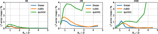
Figure 11. Mean error of  , when leaving out a value of the curvature radius
  , for the cases SE, DE and DSE (from left to right).
Download figure:
Standard image High-resolution image
Figure 12. Mean error of  , when leaving out a value of the curvature radius Rc
, for the cases DE and DSE.
, when leaving out a value of the curvature radius Rc
, for the cases DE and DSE.
Download figure:
Standard image High-resolution image4.3. Validation with an ultrasonic clamp-on flow meter
Measurements with ultrasonic clamp-on flow meters (FLEXIM FLUXUS F721) in V-path configuration have been conducted for the SE and DE with a curvature radius of  , in-between distances
 ![$d_\textrm l \in [0; 3; 4; 6] \, D$](https://content.cld.iop.org/journals/0026-1394/60/5/054002/revision4/metace7d6ieqn193.gif) , Reynolds numbers
, Reynolds numbers  and
and  , downstream distances
 ![$z \in [2.45; 5.45; 10.45; 15.45; 22.49; 25.49; 30.49; 35.49] \, D$](https://content.cld.iop.org/journals/0026-1394/60/5/054002/revision4/metace7d6ieqn196.gif) and angular orientations of
and angular orientations of ![$\varphi \in [18^{\circ}; 63^{\circ}; 108^{\circ}; 153^{\circ}]$](https://content.cld.iop.org/journals/0026-1394/60/5/054002/revision4/metace7d6ieqn197.gif) . The expanded measurement uncertainty is stated as 1%. For a detailed description of the measurement setup and the experimental determination of the calibration factors kd
, see Straka et al [29].
. The expanded measurement uncertainty is stated as 1%. For a detailed description of the measurement setup and the experimental determination of the calibration factors kd
, see Straka et al [29].
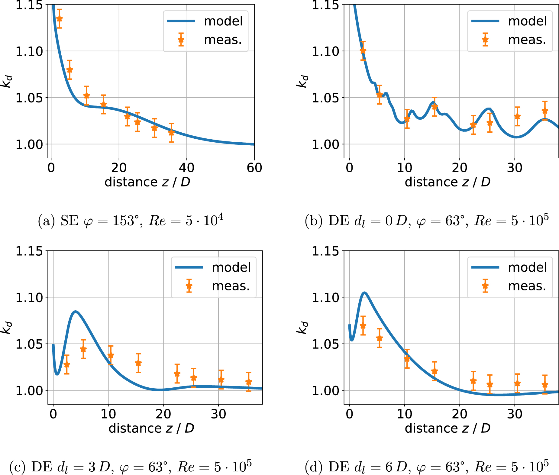
The surrogate model is evaluated with the parameters present in the measurement setup and compared to the experimental data. Figure 13 shows the calibration factor kd
over the distance z for four different parameter sets. In figure 13(a), the measurement values are in close agreement with the predicted ones, which is also true for  as shown in figure 13(b). The oscillations of kd
are stemming from the nature of the flow structure. That is, the centered single swirl, causing a rotation of the velocity profile in every downstream position and thus, the value of kd
. In figures 13(c) and (d), the prediction follows the tendency presumed by the experimental data, but misses the exact values.
as shown in figure 13(b). The oscillations of kd
are stemming from the nature of the flow structure. That is, the centered single swirl, causing a rotation of the velocity profile in every downstream position and thus, the value of kd
. In figures 13(c) and (d), the prediction follows the tendency presumed by the experimental data, but misses the exact values.

Figure 13. Correction factors kd
over the distance z with  .
.
Download figure:
Standard image High-resolution imageThe mean of the difference between the predicted  and measured
  calibration factors
  is −0.77% and the standard deviation is 1.36%. The mean of the absolute difference
  is 1.26% and the maximum absolute deviation is 4.65%. All statistics are summarized in table 3.
Table 3. Statistics of the differences between the predicted and experimental values of kd
,  .
.
| Case | SE | DE | All | |||
|---|---|---|---|---|---|---|
 Re
Re
| — | 0 | 3 | 4 | 6 | — |
| Mean of δ1 % | ||||||

| −1.16 | −1.78 | −0.77 | −0.58 | −0.71 | −0.77 |

| −0.58 | −0.79 | −0.71 | −0.40 | −0.10 | |
| STD of δ1 in % | ||||||

| 1.40 | 1.58 | 1.16 | 1.14 | 1.25 | 1.36 |

| 1.00 | 1.26 | 1.39 | 1.42 | 1.25 | |
Maximum of  in % in % | ||||||

| 3.86 | 4.65 | 2.93 | 2.96 | 3.2 | 4.65 |

| 1.62 | 3.07 | 3.20 | 3.71 | 3.42 | |
It is well known that for rotating flows, such as downstream of a DE, the strength of the swirl cannot be accurately predicted by RANS turbulence models, compare, e.g. [3, 27]. This becomes even more evident if the inflow conditions upstream of the elbows are disturbed. In consequence, the phase of the profile cannot be predicted and the evaluation of kd
for a specific angle might become biased. To overcome this issue, the angular orientation of the velocity field, respectively the angular orientation of the flow meter, can be taken as random as proposed in earlier works [34, 35]. With this approach, expected values, standard deviations and maximum/minimum bounds of kd
can be determined and used as a pragmatic prediction and estimation of the uncertainty. In figure 14, the angular mean  with its corresponding standard deviation and maximum/minimum bounds downstream of the SE is compared to the measurement data for two Reynolds numbers. It can be observed that
  is a good estimation for all angular orientations of the measurements, as most of the measurement data coincide within the standard deviation, all within the upper and lower bounds. In figures 15 and 16, the same evaluation is performed for the other parameter sets and plotted beside the measurement data for
  and
and  , respectively. Although the expected (mean) calibration factors follow the trend of the measurement data, they slightly underestimate them. Most data coincides with the maximum/minimum bounds and the uncertainty of the measurement values. An exception is the DE with
  and
and  , see figure 15(a), where the underestimation of the experimental data is more significant.

Figure 14. Mean correction factors kd
with its corresponding standard deviation, minimum/maximum error bounds and measurement data  over the distance z for the SE.
Download figure:
Standard image High-resolution image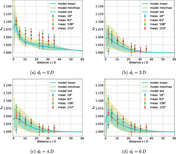
Figure 15. Mean correction factors  with its corresponding standard deviation, minimum/maximum error bounds and measurement data
  over the distance z for the DE,
  .
.
Download figure:
Standard image High-resolution image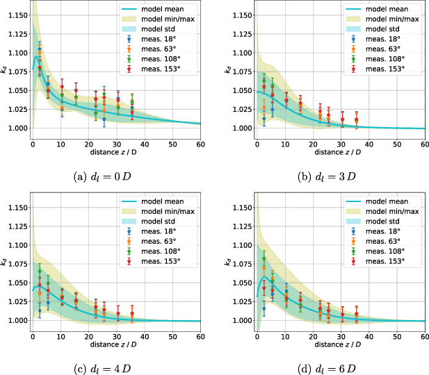
Figure 16. Mean correction factors  with its corresponding standard deviation, minimum/maximum error bounds and measurement data
  over the distance z for the DE,
  .
.
Download figure:
Standard image High-resolution image
Altogether 91.25% of the measurement data including its uncertainty range are inside the standard deviation of the model and 97.2% of the data are between the maximum and minimum bounds. The mean of the difference  is −0.78% with a standard deviation of 1.14%, whereas the mean of the absolute difference is 1.06% with a maximum of the absolute deviation of 5%. All statistics are summarized in table 4.
Table 4. Statistics of the differences between the predicted and experimental values of kd
,  .
.
| Case | SE | DE | All | |||
|---|---|---|---|---|---|---|
 Re
Re
| — | 0 | 3 | 4 | 6 | — |
| Mean of δ2 in % | ||||||

| −1.03 | −1.85 | −0.78 | −0.63 | −0.80 | −0.78 |

| −0.44 | −0.86 | −0.72 | −0.54 | −0.19 | |
| STD of δ2 in % | ||||||

| 1.00 | 1.21 | 1.18 | 1.10 | 1.41 | 1.14 |

| 0.34 | 1.07 | 1.03 | 0.90 | 1.01 | |
Maximum of  in % in % | ||||||

| 3.73 | 4.07 | 4.07 | 3.85 | 5.01 | 5.01 |

| 1.18 | 2.40 | 3.36 | 3.19 | 4.18 | |
In all parameter variations, the measurement data at the higher Reynolds number ( are closer to the model predictions. This is remarkable, as the model is based on the simulations with the lower Reynolds number (
 ). In general, the Reynolds number dependency of kd
is low.
). In general, the Reynolds number dependency of kd
is low.
5. Conclusion
In this contribution a model was developed that enables the prediction of velocity profiles and calibration factors for flow meters downstream of a SE and double elbows in- and out-of-plane. It is based on the velocity distributions from 263 CFD simulations of different geometries using the Spalart–Allmaras turbulence model. These velocity profiles were decomposed into a fully developed and disturbed part, which allowed for changing the Reynolds number and pipe wall roughness. With the method of POD the amount of data was reduced to only 5% with a maximum L2-error of less than 0.4%. Spline interpolations were performed to enable the evaluation of the model in the continuous parameter space. In a cross validation study it was shown that piecewise linear interpolation provided the most reliable results, whereas splines with higher order polynomials exhibited significant increased errors for specific parameter combinations. It could be concluded that interpolation in recirculating flows as occurring in the vicinity of an elbow exit with a small curvature radius was not reliable.
The resulting model allows real-time data evaluation with the following six parameters to choose: Reynolds number Re, sand grain wall roughness  , curvature radius
  , distance between the elbows
  , and downstream distance z. It predicts the velocity profile in the whole cross section. Hence, flow meters of different designs can be evaluated at any installation position. Calibration factors calculated for a V-path configuration of an ultrasonic flow meter were presented and compared to measurement data from an ultrasonic clamp-on flow meter. In total, 320 measurement values for five different geometries and two Reynolds numbers were considered. The comparison showed that the predicted values follow the general behaviour observed in the experimental data. However, for some parameter combinations, the predictions did not lie within the uncertainty of the measurement data. These errors can be attributed to the uncertainties of the simulation results, the surrogate model, and the flow meter model. While the exact uncertainty of each parameter combination was not determined in this contribution, it would be worth investigating in future research. Here, instead, a pragmatic approach was used to estimate the model uncertainty by treating the circumferential angle as an uncertain parameter. It was found, that the differences between the expected values and the measurement data were similar to those obtained by directly evaluating the model. Furthermore, it was demonstrated that 90% of the measurement data coincide within the standard deviations of the predictions and 97% within their maximum and minimum bounds. Therefore, the model can be used to predict calibration factors of ultrasonic flow meters within the considered range of geometry parameters. By an implementation of the model directly in a flow meter its measurement accuracy can be enhanced in disturbed conditions. Due to its cost-effective execution, another benefit of the presented model is the ability to evaluate uncertainties and sensitivities of its input parameters, e.g. by using Monte Carlo methods.
Data availability statement
The developed model can be accessed by a graphical user interface, which is available at the gitlab server of the PTB [36]. It allows the exploration of velocity profiles, the evaluation of flow meters, and the determination of uncertainties for any combination of input parameters.